Mergers and Acquisitions in Mixed-Oligopoly Markets

Mergers and Acquisitions in Mixed-Oligopoly Markets

Germán Coloma*

Department of Economics, CEMA University, Argentina

Abstract

This paper develops an oligopoly model with firms that may potentially be state-owned or privately state-owned and solves it for different cases in which the number and ownership of those firms vary. The results are then compared in terms of total surplus and consumer surplus, and this comparison produces implications for the antitrust appraisal of possible mergers and acquisitions. It follows that certain types of mergers are unambiguously favorable or unfavorable from the point of view of their contribution to both total and consumer surplus, while others may be beneficial in one of those dimensions but harmful in the other dimension.

Key words: mergers and acquisitions; mixed oligopoly; public enterprise JEL classification: L33; D43; L44

1. Introduction

The aim of this paper is to develop a model that is useful for analyzing the effect of mergers and acquisitions which occur in markets where firms can alternatively be state-owned or privately owned. The model considers the different incentives and behavioral rules that firms presumably follow, producing results that allow comparisons between the surpluses generated under different market structures and different ownership structures. The results have implications for the antitrust appraisal of mergers and acquisitions that may take place in those markets.

We assume a market for a homogeneous product that can be supplied by either one firm or two firms that interact, choosing quantities and take the quantity provided by its eventual competitor as given (Cournot oligopoly). These firms can either be state-owned or privately owned. If they are private, their objective is to maximize their profits. If they are state-owned, their objective is to maximize their managers’ utility, which we assume to be an increasing function of the firm’s

Received February 20, 2006, revised September 18, 2006, accepted October 18, 2006.

*_{Correspondence to: CEMA University, Av. Córdoba 374, Buenos Aires, C1054AAP, Argentina. E-mail:}

gcoloma@cema.edu.ar. I am grateful for the comments of Manuel Abdala, Amado Boudou, Marcelo Celani, Pao-Long Chang, Sebastián Galiani, Fernando Navajas, Martín Rossi, Jorge Streb, Mariano Tommasi, Federico Weinschelbaum, one anonymous co-editor, one anonymous referee, and participants from seminars held at CEMA University, the National University of La Plata, and the University of San Andrés.

expenditure in its production factors and inputs.

In order to make the model more tractable, we assume that market demand is linear, and the minimum average and marginal cost of providing the good supplied by the firms is constant. This permits us to analyze the results as functions of a single relevant parameter—namely, the ratio between the minimum average cost and the consumers’ reservation price (i.e., the intercept of the demand price function). 2. Related Work

The literature on antitrust analysis of mixed-oligopoly markets is notably scarce, mainly because the constituting elements of the topic have traditionally been dissociated in economic theory. Indeed, the immense majority of papers on oligopoly theory are about situations in which the suppliers are profit-maximizing private firms, and this characteristic is shared with the antitrust literature, which focuses on the normative properties of oligopoly. In contrast, the literature about public enterprise economics generally analyzes natural monopoly cases and therefore does not study the possible strategic interactions between public enterprises and their eventual private competitors.

The first academic paper of economic theory that analyzed the behavior of the mixed oligopoly seems to be Merrill and Schneider (1966). Its analysis focused on the point that, in this type of market, the introduction of a public firm may serve to implicitly regulate prices through a welfare-maximizing pricing rule set for that firm. Several years later, De Fraja and Delbono (1989) reconsidered the topic and obtained new results about the relative convenience of different structures for the mixed oligopoly, either competitive (such as Cournot) or characterized by the presence of a market leader (such as Stackelberg).

In these articles, the behavioral assumption for the public enterprise is that its objective is welfare maximization—i.e., that its positive objective coincides with its normative objective. This assumption, standard in the public enterprise literature until the early 1980s, began to change with papers such as Rees (1984) and Baumol (1984), which presented arguments about alternative positive objectives for the state-owned firm (e.g., politicians’ or managers’ utility or sales revenue). This idea became more important in the literature on public enterprise privatization that began to appear in the late 1980s; the main examples are books by Vickers and Yarrow (1988) and Bös (1991).

In this literature, the differences between the normative and the positive objectives of the public firm are explained using agency theory. This theory, however, is much more common in the literature on private monopoly regulation than in the literature on public enterprises. In Laffont and Tirole (1993), for example, there is one chapter that applies agency theory to the case of a public enterprise, but in the remaining 16 chapters, the analysis of agency questions is carried out for situations of private enterprise regulation.

The positive theory of the public enterprise, like the rest of the economic literature on state-owned companies, is mainly developed in papers that analyze

natural monopoly cases, which therefore do not consider strategic interaction issues. Recently, however, these problems began to appear in articles such as Lee and Hwang (2003) and Sappington and Sidak (2003a). In both papers, public enterprises maximize a weighted average of the surpluses of different economic agents, and that behavior is justified through agency theory considerations that explain that firms do not maximize either social welfare or private profits. These considerations also generate implications for the equilibrium prices and quantities that prevail in mixed oligopolies. In the case of Sappington and Sidak’s (2003a) article, for example, they create an incentive for the public enterprise to set prices below cost.

In another paper, Sappington and Sidak (2003b) pursue the analysis of the behavior of the mixed-oligopoly public enterprise from the point of view of antitrust policy. They raise a series of questions, which they illustrate with concrete cases, but the analysis is centered on predatory pricing issues and other exclusionary practices, and it does not enter into the topic of mergers and acquisitions.

Another recent paper with a related theme is Cook and Fabella (2002), which studies different ownership and market structures with public and private enterprises. That article, however, does not analyze the mixed-oligopoly case, since its main objective is to compare the results generated under a public monopoly with the ones that arise when that monopoly is privatized and eventually exposed to either price regulation or competition.

The main novelties of the present paper are therefore the inclusion of merger evaluation issues in the context of mixed-oligopoly markets and how that analysis differs if the acquiring or the acquired firm is state-owned. It can also be seen as a contribution to the positive theory of the public enterprise, which is simple enough to be inserted into an oligopoly model and complex enough to generate different implications under different financial, productive, and competitive constraints. Finally, we will see that the antitrust appraisal of mixed-oligopoly mergers produce different results according to the welfare definition that we use. This is particularly clear when we compare total surplus and consumer surplus criteria to evaluate mergers and acquisitions.

3. Alternative Models of Firm Behavior 3.1 Behavior of the Public Enterprise

Consider a public enterprise whose objective is to maximize its managers’ utility, and assume that the managers’ utility is an increasing function of the firm’s expenditures on production factors and inputs. This may be because managers derive utility from their remuneration while trying at the same time to minimize effort. To this end, they will increase expenditures to the highest feasible level, since reducing expenditures implies a certain effort and since part of those expenditures are used to pay for their services.

Expenditure maximization is nevertheless subject to two constraints: a financial constraint and a productive constraint. Assuming that the only source of income for

the public enterprise is sales revenue, the financial constraint implies that total expenditure cannot exceed total sales revenue, which can be written as follows:

Qg Qt P

TEg≤ ( )⋅ , (1)

where TEg is the public enterprise’s total expenditure, P(Qt) is the demand price function (its argument Qt is the total quantity traded in the market), and Qg is the quantity supplied by the public enterprise.

The productive constraint, on the other hand, has to do with the impossibility of choosing a combination of TEg and Qg for which TEg is smaller than the minimum total cost of providing Qg. This constraint is defined by the production function of Qg and the supply conditions for the production factors and inputs used by the public firm, which can be written as follows:

) (Qg

TC

TEg≥ , (2)

where TC is the total cost function of a cost-minimizing firm.

The optimization problem of the public enterprise can therefore be written in the following way:

TEg

Ug(max)= s.t. P(Qt)⋅Qg≥TEg and TEg≥TC(Qg), (3) and its solution always implies a situation where the financial constraint is binding. The productive constraint, conversely, can either be binding or not, allowing for cases where the public enterprise operates in a situation of productive inefficiency (i.e., a situation where total expenditure exceeds the minimum total cost of providing Qg).

The public enterprise’s optimization problem, therefore, can be re-written as the maximization of the following Lagrangean function:

[

( ) ( )

]

)

(Qt Qg PQt Qg TC Qg P

Lg= ⋅ +μ ⋅ − , (4)

where the financial constraint has been replaced in the objective function and in the productive constraint and μ is the Lagrange multiplier of the productive constraint. The first-order conditions for maximizing this Lagrangean with respect to Qg and

μ are: 0 ) ( ) 1 ( = ∂ ∂ ⋅ − ⎥ ⎦ ⎤ ⎢ ⎣ ⎡ ⋅ ∂ ∂ + ⋅ + = ∂ ∂ Qg TC Qg Qt P Qt P Qg Lg _{μ μ} , (5) 0 ) ( ) ( ⋅ − ≥ = ∂ ∂ Qg TC Qg Qt P Lg μ ,μ≥0,andμ

[

P(Qt)⋅Qg−TC(Qg)

]

=0, (6) and this generates two types of possible solutions: either (i) the productive constraint is not binding, μ is equal to zero, and the public enterprise chooses the quantity that maximizes sales revenue or (ii) the productive constraint is binding and the public

enterprise chooses the quantity for which the demand price equals the minimum average cost. Analytically, this is:

0 ) ( ⋅ = ∂ ∂ + Qg Qt P Qt P ⇒ sg=/η/, (7) or: 0 ) ( ) (Qt ⋅Qg−TC Qg = P ⇒ P=AC(Qg), (8)

where sg is the public enterprise’s market share (equal to the ratio of Qg to Qt ), η is the price elasticity of market demand, and AC is the minimum average cost function.

3.2 Behavior of the Private Enterprise

Let us now assume that the market under analysis can also be supplied by a profit-maximizing private firm, which is subject to the same constraints as the public enterprise. The maximization problem, therefore, can be written as:

TEp Qp Qt P

p = ⋅ −

Π (max) ( ) s.t. P(Qt)⋅Qp≥TEp andTEp≥TC(Qp), (9) where Qp is the quantity supplied by the private firm and TEp is its total expenditure on production factors and inputs.

As this firm is assumed to be a profit-maximizing one, its productive constraint will always be binding, while its financial constraint may be binding or not. This implies that the private enterprise’s optimization problem can be re-written as the maximization of the following Lagrangean function:

)] ( ) ( [ ) ( ) (Qt Qp TC Qp P Qt Qp TC Qp P Lp= ⋅ − +λ ⋅ − . (10)

The first order conditions of this problem are: 0 ) ( ) 1 ( _⎥≤ ⎦ ⎤ ⎢ ⎣ ⎡ ∂ ∂ − ⋅ ∂ ∂ + ⋅ + = ∂ ∂ Qp TC Qp Qt P Qt P Qp Lp _λ , Qp≥0, and 0 ) ( _⎥= ⎦ ⎤ ⎢ ⎣ ⎡ ∂ ∂ − ⋅ ∂ ∂ + ⋅ Qp TC Qp Qt P Qt P Qp , (11) 0 ) ( ) ( ⋅ − ≥ = ∂ ∂ Qp TC Qp Qt P Lp λ , λ≥0, and 0 )] ( ) ( [ ⋅ − = ⋅ P Qt Qp TC Qp λ , (12)

where λ is the Lagrange multiplier of the financial constraint.

This optimization problem also has two types of possible solutions. One holds when the financial constraint is not binding, λ is equal to zero, and the private firm

chooses the quantity for which its marginal revenue equals its marginal cost. The other occurs when the financial constraint is binding. This last case may imply that, at the same time, the private firm equals marginal revenue with marginal cost and price with average cost or, more probably, that it chooses Qp=0 (so that the financial constraint is satisfied in a situation where both total revenue and total cost are null). Analytically, then:

Qp TC Qp Qt P Qt P ∂ ∂ = ⋅ ∂ ∂ + ) ( / /η sp P MC P− ₌ ⇒ , (13) or: 0 = Qp , (14)

where sp is the private enterprise’s market share and MC is its marginal cost. 4. Alternative Models of Market Behavior

4.1 Mixed Duopoly Equilibrium (Case 1)

In a market with one public firm and one private firm, where each chooses its quantity by taking the other firm’s quantity as given, equilibrium occurs when we simultaneously solve equation (7) or (8) and equation (13) or (14). Which combination of these equations holds depends on the functional forms of the demand and cost functions. It is therefore useful to continue the analysis using a certain form for each of those functions and to study what happens under different parameter values.

Let us assume a linear demand function of the following form: Qt

b a

P= − ⋅ , (15)

where a and b are parameters that stand for the consumers’ reservation price and the consumers’ variation in their willingness to pay for changes in quantity. This form is probably the simplest one that generates a variable price-elasticity, which is a useful feature to assure the existence of the different types of equilibria that we are going to analyze.

Let us also assume that the total cost function is linear and that it possesses a constant average and marginal cost, given by a cost parameter c . With this assumption, we avoid the problems that have to do with the optimal number of firms in the market, and the analysis becomes centered on cases where there is not an a priori preference for monopoly or oligopoly based on cost considerations.

In the model, equilibrium depends on the ratio of c to a . If it holds that 2

1

<

a

c , this implies that equilibrium occurs when equations (7) and (13) hold simultaneously. That is:

b c a Qg ⋅ + = 3 , b c a Qp ⋅ ⋅ − = 3 2 , b c a Qt ⋅ − ⋅ = 3 2 , and 3 c a P= + . (16)

If instead c a≥12, then equilibrium occurs when equations (8) and (14) hold simultaneously, implying that:

b c a Qg= − , Qp=0, b c a Qt= − , P=c. (17)

Note that in both cases the public enterprise supplies a larger quantity than the private enterprise. This result is similar to the one obtained by Vickers (1985) for a case of a private oligopoly where revenue-maximizing firms compete against profit-maximizing firms.

4.2 Public Monopoly Equilibrium (Case 2)

Under the same assumptions about demand and costs, we obtain the equilibrium for a market with only one public enterprise and no private enterprises. If c a<1 2, this generates a situation where equation (7) is satisfied and sg=1, which implies that:

b a Qg Qt ⋅ = = 2 and 2 a P= . (18)

If, conversely, c a≥12, then equation (8) holds, and this means that:

b c a Qg

Qt= = − and P=c. (19)

Note that, in this last situation, the equilibrium is identical to the one obtained for the mixed-duopoly case. This is because, when c a≥12, the mixed duopoly becomes a public monopoly since the private firm decides not to provide the good. Note as well that, when c a<12, the public enterprise’s productive constraint is not binding, and its total expenditure is higher than the minimum total cost of providing Qg (i.e., higher than c⋅Qg). This last phenomenon also occurs in the mixed-duopoly case when c a<12. Indeed, when both the public enterprise and the private enterprise sell their product at the same price, the latter has positive profits (because its total cost is lower than its total revenue) but the former has zero profits (since it assigns all revenue to remunerate its production factors and inputs). 4.3 Private Monopoly Equilibrium (Case 3)

If we now solve the equilibrium problem for a market with a single private firm and no public enterprises, then only one solution is possible, regardless of the value of c a. This solution arises when equation (13) holds, so that:

b c a Qp Qt ⋅ − = = 2 and 2 c a P= + . (20)

Note that this solution corresponds to a situation where the private monopolist operates in an unregulated environment. This assumption about the absence of a price regulation mechanism is the same that we make for all the alternative market structures analyzed in this paper.

4.4 Private Duopoly Equilibrium (Case 4)

Let us now assume that we have a market with two private firms and no public enterprises. Then there is also one possible equilibrium outcome, which occurs when equation (13) holds for each firm. This implies that:

b c a Qp Qt ⋅ − ⋅ = = 3 ) ( 2 and 3 2 c a P= + ⋅ , (21)

where Qp is the total quantity provided by the two private firms that operate in the market, which is also supposed to be completely unregulated.

5. Efficiency Analysis

To compare the relative efficiency of the market structures described in the previous section, it is useful to define a measure of the total surplus generated in the different possible cases. That measure, denoted W , is the sum of consumer surplus (CS) and private firm profits (Πp). The public enterprise profits, which we would have to consider had we used a different model, are omitted since, in all cases under analysis, the state-owned companies operate under a binding financial constraint and they therefore obtain zero profits.

The total surplus could also encompass the surpluses obtained by people that operate inside the public and private firms (managers, workers, other suppliers, and production factors and inputs). These surpluses have also been omitted because, in this model, it is not possible to distinguish between the true social cost of production factors and inputs and the rents obtained by the suppliers of those factors and inputs.

Using the same terminology introduced in Sections 3 and 4, we can write that:

[

]

0 ( ) ( ) ( ) ( ) Qt W =CS+ Π =p ⎡_⎢ P x dx−P Qt Qt⋅ ⎤_⎥+ P Qt Qp TC Qp⋅ − ⎣

∫

⎦ ) ( ) ( ) ( 0 P xdx PQt Qg TC Qp Qt − ⋅ − =

_∫

, (22)

which, in our special case of linear demand and total cost, is equal to:

(

)

(

)

(

)

(

2 2

)

0 ₂ Qg Qp b Qp c a Qp c Qg Qt b a dx x b a W=

∫

Qt − ⋅ − − ⋅ ⋅ − ⋅ = − ⋅ + ⋅ − . (23)

Similarly, the consumer surplus generated using our linear demand function is:

(

)

(

)

2 0 ₂ Qt b Qt Qt b a dx x b a CS=

∫

Qt − ⋅ − − ⋅ ⋅ = ⋅ . (24)

Applying equation (23) to the four cases described in Section 4, we can obtain the following expressions for the total surplus corresponding to the mixed duopoly (W1), the public monopoly (W2), the private monopoly (W3), and the private duopoly (W4):

(

)

2 2 2 6 12 9 1 if , 18 2 1 1 if , 2 2 a a c c c b a W a c c b a ⎧ ⋅ − ⋅ ⋅ + ⋅ _< ⎪ _⋅ ⎪ = ⎨ − ⎪ _≥ ⎪ _⋅ ⎩ (25)

(

)

2 2 1 if , 2 2 2 1 if , 2 2 a c b a W a c c b a ⎧ < ⎪ _⋅ ⎪ = ⎨ − ⎪ _≥ ⎪ _⋅ ⎩ (26) b c c a a W ⋅ ⋅ + ⋅ ⋅ − ⋅ = 8 3 6 3 3 2 2 , (27) b c c a a W ⋅ ⋅ + ⋅ ⋅ − ⋅ = 9 4 8 4 4 2 2 . (28)

If we now apply equation (24) to the four market structures under analysis, the consumer surpluses obtained are as follows:

(

)

2 2 2 4 4 1 if , 18 2 1 1 if , 2 2 a a c c c b a CS a c c b a ⎧ ⋅ − ⋅ ⋅ + _< ⎪ _⋅ ⎪ = ⎨ − ⎪ _≥ ⎪ _⋅ ⎩ (29)

(

)

2 2 1 if , 2 2 2 1 if , 2 2 a c b a CS a c c b a ⎧ < ⎪ _⋅ ⎪ = ⎨ − ⎪ _≥ ⎪ _⋅ ⎩ (30)

(

)

b c a CS ⋅ − = 8 3 2 , (31)

(

)

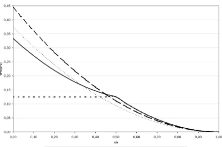
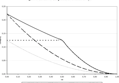
b c a CS ⋅ − ⋅ = 9 2 4 2 . (32)

a) If 0< ac <0.33, then W4>W3>W1>W2. b) If 0.33< ac <0.42, then W4>W1>W3>W2. c) If 0.42< ac <0.45, then W4>W1>W2>W3. d) If 0.45< ac <0.47, then W1>W4>W2>W3. e) If 0.47< ac <0.5, then W1>W2>W4>W3. f) If c a>0.5, then W1=W2>W4>W3. g) If 0< ac <0.35, then CS1>CS4>CS2>CS3. h) If 0.35< ac <0.5, then CS1>CS2>CS4>CS3. i) If c a>0.5, then CS1=CS2>CS4>CS3.

All these relationships arise when we compare the expressions that appear in equations (25) to (32). They can also be seen in Figures 1 and 2, which graph all the possible values of c a between 0 and 1 on the x-axis. On the y-axis, Figure 1 represents a linear transformation of W , which comes from multiplying W times

b and dividing it by 2

a . The same transformation is performed in Figure 2 for CS . This is equivalent for the special case where a= b=1.

Figure 1. Total Surplus as a Function of c a

0,00 0,05 0,10 0,15 0,20 0,25 0,30 0,35 0,40 0,45 0,00 0,10 0,20 0,30 0,40 0,50 0,60 0,70 0,80 0,90 1,00 c/a W*b/( a ^2 )

Figure 2. Consumer Surplus as a Function of c a

6. Antitrust Implications

The model presented in the previous sections carries a series of antitrust implications for merger evaluation. This is because, in markets where both public and private enterprises can operate, several important types of mergers and acquisitions can be seen as market structure modifications that consist of moving from one of the cases analyzed in this paper to another.

One example is the acquisition of a private firm by its single private competitor, which implies moving from Case 4 (private duopoly) to Case 3 (private monopoly). Another possible example is the nationalization of one of the private firms that operate in the market, which implies moving from Case 4 to Case 1 (mixed duopoly). Conversely, the privatization of a public enterprise that operates in a mixed duopoly implies moving from Case 1 to Case 4 (or to Case 3, if the acquiring firm is the public enterprise’s pre-existing competitor).

Another possible example is the nationalization of a private monopoly, which implies moving from Case 3 to Case 2 (public monopoly). Conversely, if a public monopoly is privatized, the movement is from Case 2 to Case 3. Finally, if a public enterprise that operates in a mixed duopoly acquires its private competitor, then we move from Case 1 to Case 2.

The antitrust appraisal of these seven possible situations depends on the implicit objective of the competition authority. Following the most established tradition in the international practice of competition policy, we will assume that this objective can either be total surplus maximization or consumer surplus maximization. Applying these two alternative standards, our model generates the

0,00 0,05 0,10 0,15 0,20 0,25 0,00 0,10 0,20 0,30 0,40 0,50 0,60 0,70 0,80 0,90 1,00 c/a CS*b /( a^2)

following implications for the antitrust analysis of mergers and acquisitions:

a) The acquisition of a private firm by its single private competitor reduces both consumer surplus and total surplus.

b) The acquisition of a private firm by its single public competitor also reduces total surplus and consumer surplus (unless, in the mixed duopoly equilibrium, the private firm is not producing, in which case both surpluses remain unaltered).

c) The nationalization of a private firm, when there are no pre-existing public enterprises in the market, may reduce or increase total surplus, depending on the level of productive efficiency of the private firm (i.e., on whether the ratio c a is relatively high or low). However, regardless of the efficiency level, this nationalization always increases the consumer surplus. These results are valid for cases where we move from a private duopoly to a mixed duopoly and also for cases where we move from a private monopoly to a public monopoly.

d) Similarly, the privatization of a public enterprise may also reduce or increase total surplus, depending on the ratio c a. Regardless of the value of this ratio, however, this privatization always reduces consumer surplus, and these results are valid for cases where we move from a mixed duopoly to a private duopoly, for cases where we move from a public monopoly to a private monopoly, and also for cases where we move from a mixed duopoly to a private monopoly.

Some of these conclusions are closely linked to the assumptions that we use in our model. The constant average cost assumption, for example, rules out any scale-economy argument that may lead, under exceptional circumstances, a private monopoly to generate a higher total surplus than a private duopoly. Similarly, the assumption that markets are unregulated rules out the possibility that a well-designed price regulation allows for a private monopoly to generate a higher consumer surplus than a public monopoly.

Another feature that is distinctive of our model is the fact that we do not assume that public enterprises are per se more inefficient than private firms, in contrast Lee and Hwang (2003) and Cook and Fabella (2002). This characteristic, however, can be seen as a merit of this paper, because the inefficiency of public enterprises in some market structures is an endogenous feature, produced by the interplay of a certain objective (e.g., expenditure maximization) with a series of productive, financial, and competition constraints.

Lastly, note that applying the total surplus standard or the consumer surplus standard produces the same conclusion in two cases (i.e., conclusions “a” and “b”) but different conclusions in the other five cases (conclusions “c” and “d”). This implies that it is possible that the nationalization of a private firm can be seen as beneficial because it increases consumer surplus but harmful because it reduces total surplus. Similarly, the privatization of a public enterprise can be seen as beneficial because it increases total surplus but harmful because it reduces consumer surplus.

In previous work (Coloma, 2003) we proposed, as a competition policy guideline, that the antitrust authority should prohibit those commercial practices and those mergers that simultaneously generate a reduction in total surplus and

consumer surplus, and that it should not intervene if there is a positive result in at least one of those dimensions. Applying that criterion to the analysis of the possible mergers and acquisitions described here, we state the following implications:

1) The acquisition of a private firm by its single private competitor should be prohibited.

2) The acquisition of a private firm by its single public competitor should also be prohibited (unless the private enterprise is not operating).

3) The nationalization of a private firm should not be prohibited if the pre-existing market structure is a private duopoly or a private monopoly.

4) The privatization of a public enterprise should not be prohibited, either, unless it occurs in a situation where the expected productive efficiency gain is negligible.

References

Baumol, W., (1984), “Toward a Theory of Public Enterprise,” Atlantic Economic Journal, 12, 13-19.

Bös, D., (1991), Privatization: A Theoretical Treatment, Amsterdam: North Holland. Coloma, G., (2003), Defensa de la Competencia, Buenos Aires: Ciudad Argentina. Cook, P. and R. V. Fabella, (2002), “The Welfare and Political Economy

Dimensions of Private versus State Enterprise,” Manchester School, 70, 246-261.

De Fraja, G. and F. Delbono, (1989), “Alternative Strategies of a Public Enterprise in Oligopoly,” Oxford Economic Papers, 41, 302-311.

Laffont, J. J. and J. Tirole, (1993), A Theory of Incentives in Procurement and Regulation, Cambridge: MIT Press.

Lee, S. H. and H. S. Hwang, (2003), “Partial Ownership for the Public Firm and Competition,” Japanese Economic Review, 54, 324-335.

Merrill, W. and N. Schneider, (1966), “Government Firms in Oligopoly Industries: A Short-Run Analysis,” Quarterly Journal of Economics, 80, 400-412.

Rees, R., (1984), “A Positive Theory of the Public Enterprise,” in The Performance of Public Enterprises, M. Marchand, P. Pestieau and H. Tulkens eds., Amsterdam: North Holland, pp. 179-191.

Sappington, D. and G. Sidak, (2003a), “Incentives for Anticompetitive Behavior by Public Enterprises,” Review of Industrial Organization, 22, 183-206.

Sappington, D. and G. Sidak, (2003b), “Competition Law for State-Owned Enterprises,” Antitrust Law Journal, 71, 479-523.

Vickers, J., (1985), “Delegation and the Theory of the Firm,” Economic Journal (Supplement), 95, 138-147.

Vickers, J. and G. Yarrow, (1988), Privatization: An Economic Analysis, Cambridge: MIT Press.