INFORMATION SCIENCES 7&l-34 (1993)
Optimal Assignment of Task Modules with Precedence in Distributed Computing Systems
GEN-HUEY CHEN
Department of Computer Science and Information Engineering, National Taiwan University Taipei, Taiwan, Republic of China and
JYH-SHIARN YUR
Institute of Information Engineeting Tatung Institute of Technology, Taipei, Taiwan, Republic of China
ABSTRACT
We consider the problem of finding an optimal assignment of task modules with a precedence relationship in a distributed computing system. The objective of task assignment is to minimize the task turnaround time, i.e., the total time required to finish the execution of a task. This problem is known to be NP-complete for more than three processors. To solve the problem, a well-known state space reduction technique, branch-and-bound-with-underestimates, is applied, and two underestimate functions are defined. Through experiment, their effectiveness is shown by comparison with both Wang and Tsai’s algorithm and the A* algorithm. Parameters considered in the experiment include the number of modules, the number of processors, the ratio of average intermodule communication time to average module execution time, and the shapes of task graphs. Statistical data about the number of search nodes, maximal queue length, and execution time are collected for performance evaluation.
1. INTRODUCTION
The rapid progress of microprocessor technology has made distributed computing systems economically attractive for many computer applica- tions. In a distributed computing system, a task (program) may be dis- tributed among processors to speed up execution by taking advantage of
Correspondence to Prof. Gen-Huey Chen.
OElsevier Science Publishing Co., Inc. 1993
system computation abilities and resources. However, the overall system performance is dependent on many factors; among them, the most crucial one is the assignment of task modules to processors. In general, a task can be suitably divided into a set of interdependent tusk modules (modules, for short) that can be executed on the processors of the distributed computing system. The cost of executing a module may vary from processor to processor. During task execution, some control messages and intermediate data are required to be transmitted among modules. Two communicating modules that are executed on different processors consume a system’s communication resource, and thus incur a communication cost because of the overheads due to the communication protocols and transmission delays in the communication subnetwork. Here, cost values are defined in terms of a single unit, time. Hence, the total time, called the tusk turnaround time, required to finish the execution of the entire task is composed of the module execution time (MET), intermodule communication time (ZCT), and processor idle time (PIT 1.
Our attention for task assignment is focused on finding an optimal assignment that minimizes the task turnaround time. To achieve this objective, we need to balance the computation loads of the processors, and at the same time minimize the intermodule communication overheads. This problem for more than three processors is known to be NP-complete [2]. Solution methods already suggested for the problem can be roughly classified into four categories: graph-theoretic approaches [ill, [151, [16], integer O-l programming approaches [5], [12], [13], [19], heuristic approaches [61,[81, and simulated annealing approaches [18]. Stone [151 has solved the problem by partitioning the processor-module flow graph using a max-flow min-cut algorithm. Modeling the problem as a combinatorial optimization problem, integer O-l programming approaches use mathe- matical optimization techniques to search for an optimal assignment. Instead of pursuing an optimal solution, heuristic approaches find near- optimal solutions by applying some heuristic strategies. Simulated anneal- ing approaches use stochastic search criteria to refine an initial solution to a globally optimal solution in finite iterations.
Wang and Tsai [19] formulated the task assignment problem as a graph matching problem, and then presented an A* algorithm [lo] to search for an optimal assignment. Their algorithm has worse performance when the intermodule communication time is relatively small (compared with the module execution time). In this paper, we propose a new algorithm for the task assignment problem that behaves very well in that case. In our algorithm, a well-known state space reduction technique, brunch-and- bound-with-underestimates (BZ?U), is applied, and two underestimate func- tions, fMETu and far”, are defined. To show the effectiveness of our
OPTIMAL ASSIGNMENT OF TASK MODULES 3 algorithm, statistical data about the number of search nodes, maximal queue length, and execution time are generated. Parameters considered in our experiment include the number of modules, the number of processors, the shapes of task graphs (defined in the next section), and the ratio of average intermodule communication time to average module execution time.
The remainder of the paper is organized as follows. In Section 2, system assumptions are stated and the task assignment problem is formulated. In Section 3, two underestimate functions, fMETLT and fATLI, are defined and a BBU algorithm is proposed. In addition, an initial feasible solution is suggested for our algorithm, and some state space reduction rules are introduced. They can fathom more search nodes during the state space search. Experimental results are shown in Section 4. Finally, concluding remarks are given in Section 5.
2. ASSUMPTIONS AND PROBLEM STATEMENT 2.1. ASSUMPTIONS
The task assignment problem we consider in this paper has the same assumptions as Wang and Tsai have made in [19].
(1) The processors in the distributed computing system are heteroge- neous.
(2) All processors can communicate with each other through the com- munication subnetwork.
(3) All communication links are symmetric. That is, transmission on both directions of a communication link takes the same time. But, trans- mission on different communication links may take different times.
(4) Synchronization between two communicating processors is neces- sary before starting message transmission (i.e., message transmission and module execution cannot be overlapped). This means that the two commu- nicating processors spend the same amount of communication time, but one of them may incur additional idle time.
(5) There exists a precedence relationship among modules. It speci- fies the feasible execution sequences of modules. No cyclic precedence relationship is allowed among modules.
2.2. PROBLEM STATEMENT
There are m modules M,, M2, . , . , Mm contained in a given task. The task can be conveniently represented by an acyclic directed graph, called
the tusk graph, as follows. Each module of the task is uniquely represented by a vertex of the task graph, and there is an arc from Mi to Mj if and only if message transmission is needed from M, to Mj (i.e., Mi precedes Mj) during the task execution. Again, the task graph can be represented by an m x m adjacency matrix TSK; TSK(i, j) = 1 if there is an arc from Mi to Mj and TSK(i, j) = 0 otherwise. If the modules are arranged in a topological order [7] according to their precedence relationship, then TSK is an upper triangular matrix. In subsequent discussion, we consider TSK upper triangular.
If there exists a path from M, to Mj in the task graph, then Mi is called a predecessor of M,, and Mj is called a successor of Mi. If there exists an arc from Mi to Mj, then IV, is called an immediatepredecessor of Mj, and Mj is called an immediate successor of Mi. A module without any successor is called a sink module, and a module without any predecessor is called a source module. A module is not allowed to start execution until all of its immediate predecessors have finished execution.
There are n processors P,, P2,. . . , P,, in the distributed computing system. Let MET(i, j) denote the module execution time required for executing M, on P,, and let ZCT(a, b, i, j) denote the intermodule commu- nication time required for the pair of modules M, and Mb when they are assigned to Pi and Pj, respectively. Since symmetric communication links are assumed, ZCT(a, b, i, j) = ZCT(a, b, j, i). Moreover, it is also assumed that ZCT(a, b, i, j) = 0 if i = j.
Let PT(i) denote the processor turnaround time of Pi, which is the total time consumed on Pi. When the task finishes its execution, the maximal processor turnaround time is the task turnaround time. The task assignment problem is to find a mapping from the task graph to the distributed computing system which minimizes the task turnaround time subject to the precedence constraint.
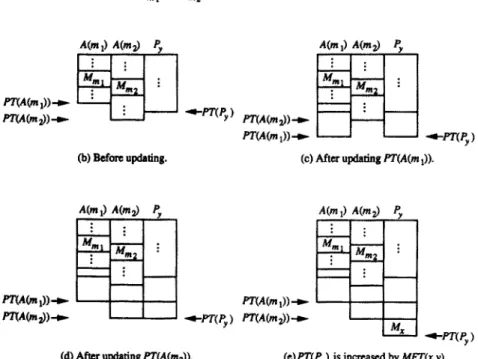
During the execution of our algorithm, processor turnaround times are updated whenever a module, say M,, is assigned to a processor, say Py. Suppose M,,,,, M,,,,, . . . , M,,,, are immediate predecessors of M,, and they are arranged in nondecreasing order of processor turnaround times. That is PT(A(mi)) Q PT(A(mj)) for 1 <i <j G k, where A(mi) denotes the processor to which M,,,, is assigned. PT(A(m,)), PT(A(m,)), . . . , PT(A(m,)) need to be updated when M, is assigned to Py. The updating proceeds in the order of PT(A(m,)), PT(A(m,)), . . . , PT(A(m,)). To update PT(A(mi)), 1 <i <k, processors P, and A(mi) are first synchronized, and then spend the same amount of time for message transmission. Finally, after finishing the updating of PT(A(mi))‘s, i = 1,. . . , k, PT(P1) is increased by the module execution time of M, on P,. The detailed procedure is shown in Algorithm 1.
OPTIMAL ASSIGNMENT OF TASK MODULES 5 Algorithm 1
/* Update the processor turnaround time. */
Step 1. /* Suppose that Mm1,Mm2,. .., Mm, are arranged in nonde- creasing order of processor turnaround time, i.e., PT(A(m,)) <PT(A(mj)) for 1~ i <j G k, and A4, is assigned to PY. */
for (i=l; i<=k; i-t+) I
PTMm,N =mdPT(y), PTMm,)N + Kmm,, x, A(mJ y); PT(y) = PTL4bq));
Step 2. PT(y) = PT(y) +MET(x, y).
Algorithm 1 takes O(k) time. In Figure 1, the execution of Algorithm 1 is illustrated by an example.
3. STATE SPACE SEARCH REDUCTION
In this section, a branch-and-bound-with-underestimates (BBU) algo- rithm is presented to find an optimal solution for the task assignment problem. The state space graph of a BBU algorithm is a search tree whose nodes each, except for the root node, correspond to an assignment of a module to a processor. Associated with each node x in the search tree is a partial assignment A, that consists of all of the module-to-processor assignments of the nodes along the path from the root to X. By A,(i) = j we denote that module Mi is assigned to processor Pj in the partial assignment A,. Associated with each node x is also an underestimation f(x) =g(x) +/z(x) of the minimal task turnaround time caused by the
complete assignments that include A, as a part. The value g(x) is the maximal processor turnaround time caused by A,, and h(x) is an underes- timation of the minimal processor turnaround time that will be incurred from node x to a goal node. A goal node is a node that represents a complete assignment. One simple, but inaccurate, way to compute f(x) is to let h(x) = 0. The accuracy of h(x) greatly affects the efficiency of a BBU algorithm. Besides, an upper bound cost (UC) is associated with a BBU algorithm, and it represents an upper bound on the minimal task turnaround time. The value UC is set infinity initially, and is updated to min{UC,f(z>) whenever a goal node z is reached.
(8) M,,,, ad M,,,,m immediate prtxiwc~
oft, .
A(mJ A(mz) 5
I
H
(b) Bcforc updating.(d) Afm updating pT(AC2)). (e)P?‘(pY ) is incrwcd by MW(xy).
Fig. 1. The updating of processor turnaround times.
A list, called the u~~~a~ded &, is necessary for a BBU algorithm to store all unexpanded search nodes from which it is still possible to find an optimal assignment. Initially, the unexpanded list is empty. The BBU algorithm begins with placing the root node into the unexpanded list. The root node corresponds to the null state (no modules assigned). During the state space search, a search node x with minimal underestimation f(x) is always selected from the unexpanded list to be expanded next. Let those unassigned modules whose predecessors have all been assigned be referred to as ready modules. If x is not a goal node, n possible assignments Mi to z$j=l,..., n, for each ready module Mi are checked for their feasibilities
OPTIMAL ASSIGNMENT OF TASK MODULES 7 (it will be seen later in this section that some constraints may be derived during the state space search), and a child node is generated for each of the feasible assignments. Then, for each generated child node y, the underestimation f(y) is computed. If f(y) < UC, node y is inserted into the unexpanded list. Otherwise, node y is fathomed since further expan- sion form it will not lead to an optimal solution. All nodes in the unexpanded list are maintained in nondecreasing order of underestima- tions. If the selected node x is a goal node, the algorithm terminates since it is impossible to find a better solution from the other nodes.
In the rest of this section, we first briefly review Wang and Tsai’s algorithm [19], and then introduce two underestimate functions f,,,sro and
f
ATU’3.1. A BRIEF REVIEW OF WANG AND TSAI’S ALGORITHM
The essence of Wang and Tsai’s algorithm [19] is to underestimate the minimal task turnaround time from the viewpoint of the bottleneck proces- sor. The bottleneck processor is the processor with the maximal processor turnaround time. In their algorithm, the minimal task turnaround time is underestimated for each partial assignment by summing up the minimal time required for each of the unassigned modules that need to communi- cate with those modules that have been assigned to the current bottleneck processor.
For a partial assignment A,, let us define the following notations: Pb: the bottleneck processor;
Li: the set of modules assigned to processor Pi;
Q: the union of Li’s, i.e., the set of all assigned modules; Q’: the set of all unassigned modules;
S: the set of modules in Q’ that communicate with modules in L,. Wang and Tsai’s algorithm computes h(x) as the summation of Hg for all M4 in S, where
H,=min{t,t’},
t=Mx(q,b) +
c
~Cqbq>~,(r),q,
rEQ-Lb andand t’= min p=l,...,n i c ZCT(r,q,b,p) rsL, and TSK(r,q)= 1
The computation of t assumes that Mg is assigned to Pb, and the computation of t’ assumes that Mg is not assigned to Pb. In essence, Wang and Tsai’s algorithm computes h(x) from the viewpoint of proces- sors, which is the main reason for a poor underestimation as the intermod- ule communication time is relatively small (compared with the module execution time). It thus motivates us to revisit the problem from the viewpoint of modules.
3.2. MINIMAL EXECUTION TIME UNDERESTIMATE (METU)
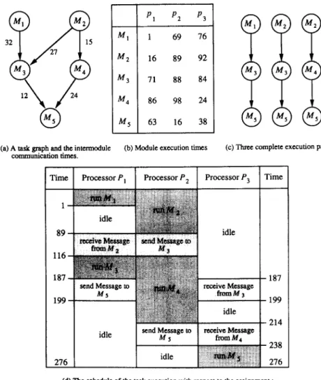
Given a task graph, the task starts execution from source modules and terminates after all sink modules are finished. A directed path from a module Mi to a sink module Mj is called an execution path, and is called a complete execution path if Mi is a source module. The execution time of an execution path from Mj to Mj is defined to be the time length from the time when Mi starts execution to the time when Mj finishes execution. The execution time of an execution path contains the module execution times, the intermodule communication times, and the processor idle times that must be spent to finish the execution of the execution path. There may be a number of complete execution paths contained in the task graph. With respect to a mapping from the task graph to the set of processors, we define the critical complete execution paths as those complete execution paths whose execution times are equal to the task turnaround time. In Figure 2, an example is shown where the given task graph [see Figure 2(a)] contains three complete execution paths [see Figure 2(c)]: (M,,M,, M,), (M,,M,,M,), and (M,,M,,M,). Also, note that for any two modules, uniform intermodule communication times are assumed in Figure 2. That is, for two communicating modules n/r, and Mb, ZCT(a, b,i,jYs are the same for any i #j. For the assignment M, to P,, M2 to P.,, M3 to P,, M4 to P2, and M5 to P3, the execution time of each of the three complete execution paths is 276 [see Figure 2(d)], which is the task turnaround time. So, they are all critical complete execution paths with respect to the designated assignment.
Based on the concept of execution paths, two underestimate functions,
f
METU and fAT" (fATi is defined in the next subsection), are therefore proposed.OPTIMAL ASSIGNMENT OF TASK MODULES 9 M, Ml M3 M4 MS 1 69 76 16 89 92 71 88 84 86 98 24 63 16 38
(a) A task graph and the intermodule (b) Module execution times (c) Three complete execution paths.
Yime Processor P,
I Processor P 2 Processor P, Time
.187
.214 .238 276
(d) The schedule of the task execution with nspect to the assignment : Mt’OP,,M2to~,M~tOl;,Uq~~,and~~toP,.
Fig. 2. An illustrative example.
For an arbitrary execution path CM,,, M+. . . , Mi,> extended from M,,, the summation
,$ ,=yJ n IMWi,J+} , 1
is an underestimation of the execution time for the execution path. For each module M,, we define MAXET(1’) to be the maximum of the underes-
timated execution times for all of the execution paths that are extended from the immediate successors of Mi. Clearly, if Mi is a sink module, MAXET(i) = 0. Otherwise, MAXET(i) is computed recursively as
max
M, is an immediate S”CCeSSOr of M,
All of the values MAxET(i) are determined prior to the execution of the BBU algorithm. The time complexity for computing all MAXET(i)‘s are @en), where e is the number of arcs in the task graph. In Table 1, we show the values of MAXET(i)‘s for the example of Figure 2. For example, MAxET(2) = mux{MAXET(3) + 71, MAxET(4) + 24) = mux{87,40) = 87.
Let us consider a partial assignment A, that is associated with a search node x during the execution of the BBU algorithm. With respect to A,, as before, denote the set of all assigned modules by Q and the set of all unassigned modules by Q’. Since the value MAxET(i) is an underestima- tion of the time required to finish the execution of all successors of Mi, we can define an underestimate function f&, as follows:
f
ifmu =
mux
Mi is in Q and all
{PT(A,(i)) +MAXET(i)). immediate successors of
M, are in Q’
In the above formula, PT(A,(i)) is the current processor turnaround time of the processor where Mi is resident. It also represents the time when the execution of Mi and all of its predecessors is finished. The computation of
fhETrr
(x)
is to underestimate the task turnaround time with respect to the partial assignment A, by underestimating the time required to finish the execution of all successors of Mi as MAXET(i). Note that since MAXET is defined for all immediate successors of Mi, they must be not yet assigned with respect to the partial assignment A,.TABLE 1
The values of MAxET(i)‘s for the example of Figure 2
i 1 2 3 4 5
OPTIMAL ASSIGNMENT OF TASK MODULES 11 Also note that the computation of &r&l ignores the processor synchronization and the intermodule communication time caused by M, and its immediate successors. To obtain a more accurate estimation of the task turnaround time, we have to take these two factors into consideration. Hence, the assignment of the immediate successors of Mi should be considered. The resulting underestimate function is f,,,,(x), which is defined as follows:
f
MEW(X)
= ma
M, is in Qi
{m~{PT(A,(i)),PT(p)}
+ZCT(i, j,A,(i),p) +MET(j,p)
+~ZWi)})
i
.
In the above formula, the term mux{PT(A,(i)),PT(p)) indicates the synchronization between the two communicating processors where Mi and Mj are assigned, respectively, and its value represents the time when Mi and iVj are allowed to start message transmission. Since the execu- tion of Mi and all of its predecessors is finished by this time, the value min,=,,,,, ,{mm{PT(A&)), PT(p)} + ZCT(i, j, A,(i), p) + MET (j, p) + MET( J ‘11 is an underestimation of the time required to finish the execution of all predecessors of Mi, Mi, Mj, and all successors of Mj. The computation offMsTu
(x)
is completed by calculating this value for each Mi in Q and each immediate successor Mj of Mi, and then taking the maximum as an underestimation of the task turnaround time with respect to the partial assignment A,. If it4, is a sink module, the value of the term mux{min{max(. ..) + -*e)) is computed as PT(A,(i)).Assume that there are k modules in Q, and that they contain r1,r2,..., r,, respectively, immediate successors in Q’. The time complexity of computing
f,,,,<x>
is O((r, + r2 + +-- +r,>n).3.3. ASSIGNMENT TREE UNDERESTIMATE (4 TU)
The underestimate function
fMsTu
does not fully consider the inter- module communication time that will be spent along an execution path. We take this factor into consideration in the underestimate functionfATU.
In essence, fAru determines how to assign the modules along a complete execution path such that the sum of the module execution time and the intermodule communication time is minimized. Thus, finding an optimal assignment of modules along each complete execution path forms the central part of the fAru function.
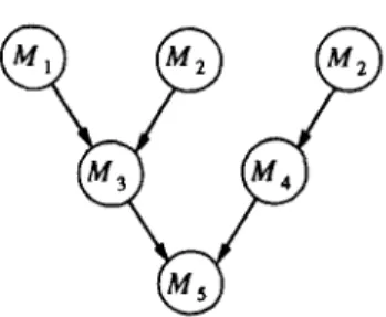
Before defining the f’ru function, we describe the construction of execution trees from a task graph. The execution trees are rooted at sink modules and grow upward. Each node of an execution tree represents (probably not uniquely) a module. Module A4, is an immediate predecessor of module Mj in the task graph if and only if there is a node corresponding to A4, which is a child node of a node corresponding to Mj in the execution trees. Thus, each path from a leaf node to a root node in the execution trees forms a complete execution path, and all complete execution paths appear exactly once in the execution trees. There is the same number of execution trees as sink modules. The execution trees for the example of Figure 2 are shown in Figure 3. Note that module M2 is represented by two nodes in Figure 3.
Based on the execution trees, we can build assignment trees. Each assignment tree is built from an execution tree by considering the assign- ment of the corresponding modules of the nodes in the execution tree. Each node of an assignment tree contains n subnodes consisting of the n possible assignments of its corresponding module. Each edge in the execution trees is replaced by n in links in the assignment trees. These links represent all possible assignments of two communicating modules. In Figure 4, a part [corresponding to the complete execution path (1,3,5)] of the assignment tree built from Figure 3 is shown, where the notation “i -j” represents “assigning module M, to processor Pj.” For example, the dashed line connecting nodes 7 and 9 means that M3 and M5 are assigned to P3 and P2, respectively. The bold lines in Figure 4 represent the assignment of M, to P,, M2 to P2, M3 to P,, M4 to P2, and M5 to P3.
OPTIMAL ASSIGNMENT OF TASK MODULES 13 \ \ \ \ \ \ / / / / / \ \ \ \ / , \ \
Associated with each node in the assignment trees are some variables which are necessary in defining the underestimate function fATU. For the convenience of the description, we collect these variables in a C-type data structure as follows.
typedef struct node 1
int module;
int no-child;
unsigned exe_time[ NO_PROC][ NOJ’ROC]; unsigned min_exe_time[ NO_PROC]; struct node *parent;
INODE;
The identifier NO-PROC is a constant denoting the number of proces- sors in the distributed computing system. The identifier module is a variable denoting the module represented by the node. The module M, is considered a dummy module, and a node representing a dummy module is considered a dummy node. For example, node 1 in Figure 4 is a dummy node. The dummy node acts as the head of a complete execution path. The identifier no-child is a variable giving the number of child nodes (equal to the number of immediate predecessors of the associated module). The identifier parent is a pointer to the parent node. A node representing a sink module has its parent equal to NULL. The identifiers exe-time and min.-exe-time will be explained later.
From Figure 4, it is seen that the assignment trees consider all possible assignments of modules along each complete execution path. Therefore, a specific assignment of modules along a complete execution path corre- sponds to a path from a dummy node to a root node in the assignment trees. Links of the assignment trees are weighted with intermodule com- munication times, and their nodes are weighted with module execution times. Ah links incident to a dummy node have their weights equal to zero. Unlike the execution time of an execution path in the task graph, let us define the execution time of a path from a node to a root node in the assignment trees as the sum of the module execution times and the intermodule communication times along that path, exclusive of the module execution time of the starting node. For example, in Figure 4, the execution time of the path (O-3,1-3,3-3,5-2) is O+MET(1,3)+O+MET(3,3)+ ICT(3,5,3,2) +MET(5,2) = 188, and the execution time of the path
(2-2,3-3,5-2) is ZCT(2,3,2,3) + MET(3,3) + ZCT(3,5,3,2) + ME7’(5,2) = 139.
Consequently, determining an optimal assignment of modules along a complete execution path which minimizes the sum of the module execu-
OPTIMAL ASSIGNMENT OF TASK MODULES 15 tion times and the intermodule communication times is equivalent to determining a shortest path from a dummy node to a root node in the assignment trees, which can be done by aid from the values min_exe_time[i]‘s and exe_time[i][jj’s that are stored in nodes of the assignment trees.
For each node in Figure 4, the values in parentheses represent the variables e.xe_time[i][j]. They denote the execution times of the shortest paths from the node to the root node if the associated module and the module associated with its parent node are assigned to Pi+ i and Pj+ 1, respectively (note that the array index of C language starts from 0). Also in Figure 4, the values in square brackets represent the variables min_Rue.-time[i]. They denote the execution times of the shortest paths from the node to the root node if the associated module is assigned to pi+,* Clearly, mia_ere_time[i] = minj= O,_.,,r? _ ,{~e-~~~~[~][~]]. For example, node 4 in Figure 4 considers the assignment of module M, along the complete execution path (1,3,5). The value 136 in the parentheses under l-l is the content of exe_time[O][l], and it represents the execution time of the shortest path from node 4 to the root node if M1 and its immediate successor N, are assigned to P, and Pz, respectively. The value 99 in the square brackets is the content of min_exe_time[O], and it represents the execution time of the shortest path from node 4 to the root node if M, is assigned to P,. Recall that the module execution time of the starting node is excluded in the execution time of a path in the assignment trees.
The assignment trees are established before the BBU algorithm starts execution. By applying Bokhari’s shortest tree algorithm [2], the values min_exe_time[i] and exe_time[i][j] can be computed. These values can be used to find a shortest path from an arbitrary node to a root node in the assignment trees (equivalent to determining an optimal assignment of modules along an execution path), which is the most essential step in computing f,,,(x).
Since the assignment trees are obtained from the execution trees, they also retain the precedence relationship among modules. Let us consider a complete execution path in the task graph. Assigning modules along the complete execution path can be regarded as choosing a path from a dummy node to a root node in the assignment trees. A complete (partial) assignment along the complete execution path corresponds to a traveling tour that contains the entirety (a part) of the corresponding path in the assignment trees. Here, a complete (partial) assignment along a complete execution path refers to an assignment of all (a subset of) the modules contained in the complete execution path.
Since any node x in the search tree represents a partial assignment A,, we can associate an array of pointers, named trace!, with the node x to
represent the traveling tours that correspond to A,. Moreover, since A, can be regarded as a union of all of the partial assignments consistent with A, along all complete execution paths in the task graph, the length of travel is equal to the number of complete execution paths, and each pointer in trauel is responsible for keeping track of a traveling tour of a dummy node to root node path in the assignment trees. In our BBU algorithm, each pointer in travel always points to the frontier of a traveling tour, that is, the node (of the assignment trees) whose associated module was assigned last along a dummy node to root node path. For example, let us consider the example of Figure 2. If three modules, M,, M2, and M4, have been assigned in the partial assignment A,, then the pointers in travel of node x point to nodes 4, 5, and 8, respectively, in Figure 4.
At the beginning of the BBU algorithm, the pointers in travel of the root node point to the dummy nodes of the assignment trees because all modules are not yet assigned. During the execution of the BBU algorithm, whenever a search node x corresponding to, for example, the assignment of module MO to processor Pb is generated, the array travel of node x is constructed as follows. First, a copy of travel is gotten from the parent node of X. Then, a pointer in travel is moved down to the next node (in the assignment trees> toward the root node if the module associated with the next node is M,. If multiple pointers point to the same node, only one of them is kept. For example, let us consider the example of Figure 2 again. Suppose three modules, M,, M2, and iW4, are assigned in the partial assignment A,, and the pointers in travel of node x point to nodes 4, 5, and 8, respectively, in Figure 4. If a node y that corresponds to the assignment of M3 is generated as a child node of x during the execution of the BBU algorithm, then the array travel of node y is constructed as follows. First, a copy of travel is gotten from node x. Then the two pointers to nodes 4 and 5, respectively, are moved down to node 7 because the module associated with node 7 is M3. Further, since they both point to the same node after movement, only one of them is kept. The pointer to node 8 remains unchanged.
A more detailed description of constructing the array travel for a newly generated search node x is shown in Algorithm 2.
Algorithm 2
/* Construct the array travel for a newly generated search node X. Assume that the node x corresponds to the assignment of module it4, to processor Pb. The variable t saves the number of pointers in travel. The
OPTIMAL ASSIGNMENT OF TASK MODULES 17 array no_pred is a global variable, and no_pred[i] denotes the number of immediate predecessors of module Mi. */
for(i=l,j=O; i<=t; i++) 1
next = truvel[il - >parent;
if (next ! = NULL && next - > module == a) next - > no-child - - ;
/* Are there multiple pointers to the node next? */ if (next - > no-child > = 1) continue;
traveZ[ i 1 = next;
/* Restore the value of no-child */
next - > no-child = no_pred[ next - > module]; /* Pack the pointers */
traveZ[ ++jl = traveZ[iI; t =j.
The time complexity of Algorithm 2 is O(t). Now, based on the above discussion, we define an underestimate function f;,,(x) for a partial assignment A, that is represented by a search node x:
fLTv( x) = i=yx
,...,f {PT( A,( trauel[ i] - > module))
+travel[i] ->min_exe_time[ A.(travel[i] ->module) - 11). In the above formula, the value t denotes the number of valid pointers in travel, and decreasing the index of min_txe_time by 1 is due to the array index of C language starting from 0. If travel[i] - >module is a dummy module, then PT(A,(travel[i] - >module)) is set to 0, and A,(truvel[i] - > module) can be any of 1,2,. . . , It. If truvel[i] - > module is not a dummy module, say Mk, then PT(A,(R)) is the time when Mk and its immediate successors can start message transmission (i.e., the time when the execution of Mk and all of its predecessors is finished). The value truvel[i] - > min_exe_time[ A,(k) - 11 is taken as an underestimation of the time required to finish the execution of all successors of Mk along the path from the node pointed at by travel[i] to the root node. The value f;,,(x) underestimates the task turnaround time with respect to the partial assignment A, by taking travef[il - > min_exe_time[ A,(k) - 11 as an underestimation of the execution time of the path from the node
pointed at by truuel[i] to the root node. For example, let us consider Figure 4 again. If only module M3 and all of its predecessors have been assigned, then there is a pointer, say truvel[i], to node 7. Now, PT(A,(truuel[i] - > module)) =PT(AX(3)) is the time when the execution of iVfJ and all of its predecessors is finished, and truuel[i] - > min_exe_time[A,(3) - l] is an underestimation of the time required to finish the execution of M,. Thus, PT(A,(3)) + truvel[i] - > min_exe_time[A.(3) - l] is an underestimation of the time required to finish the execution of all predecessors of M,, M3, and M,.
Note that the computation of f& (x1 ignores the processor synchro- nization and the intermodule communication time caused by the module truvel[i] - > module and its immediate successor truuel[ i] - >purent - > module. To make a more accurate estimation of the task turnaround time, we have to take these two factors into consideration. Hence, the assign- ment of the module truuel[ i] - >purent - > module should be considered. The resulting underestimate function is fAT&x), which is defined follows:
fAT”(X)
=
max ( min { mux PT Ai=l,..., f p=l,..., n { ( x( trauel[i]->module)),PT(p)}
+truuel[ i] - > exe_time[ A,( truuel[ i] - > module) -
[P-q).
as
11
In the above formula, Pp is the processor where the module travel [i] - >purent - >module is attempted to be assigned. The term mux (PT( A,(truvel[i] - > module)), PT( p)} indicates the synchronization between the two communicating processors where the module truvel[i] -
> module and the module truuel[ i] - >purent - > module are resident, and its value represents the time when the two modules can start message transmission. If truuel[i] - > module is a dummy module, then PT(A, (truuel[i] - > module)) is a set to 0 and A,(truuel[ i] - > module) can be any of 1,2,..., n. If truvel[i] - > module is a sink module, then no immediate successor of it exists and PT(p) is set to 0. The value truvel[i] - > ae_time[ A,(truuel[i] - > module) - l>][ p - 11 is taken as an underestima- tion of the time required to finish the execution of all successors of the module truuel[i] - > module along the path from the node pointed at by truuel[i] to the root node. The value
fATu(x)
underestimates the task turnaround time with respect to the partial assignment A, by takingOPTIMAL ASSIGNMENT OF TASK MODULES 19 truuel[i] - > exe_time[ A,(truuel[ i I- > module) - l][ P - 11 as an underesti- mation of the execution time of the path from the node pointed at by truuel[i] to the root node.
The time complexity of computing f&x) is 0(&z>, where t denotes the length of truuel. The space requirement depends on both the maximal length of the unexpanded list and the number of nodes in the assignment trees.
3.4. AN INITIAL SOLUTION
For a BBU algorithm, a good enough initial solution can save much computation and memory by fathoming nodes at the beginning of the state space search. For the task assignment problem, there is a trivial solution, i.e., assigning all modules to the same processor. In fact, our experiment shows that the trivial solution is almost an optimal solution when the intermodule communication time is much greater than the module execu- tion time. On the other hand, the trivial solution is bad when the module execution time is greater than the intermodule communication time. For the latter case, an algorithm using the concept fATU is applied to find a good enough initial solution. A similar algorithm using the concept of
f METU
can also be derived easily.Initially, let truuel[i]‘s point to dummy nodes. Associated with each truuel[il, let us define Hi) as follows:
E(i) = p=ryin {mux{PT(A,(rruuel[i] ->module)),PT(p)} ,...,a
+truuel[i] ->exe_time[A,(truuel[i] ->module) -11
[P--11}.
In the above formula, Pp is the processor where the module travel [i] - >purent - >module attempts to be assigned. The value E(i) is an underestimation of the time required to finish the module fruuel[i] - > module, all of its predecessors, and its successors along the path from the node pointed at by truuel[i] to the root node.
Also, let UG, b) denote mux{PTL4,hzuel[iI - > module)), PT(b)) + truuel[i] - > exe_time[ A,(truuel[il - > module) - l)l[b - 0, which is an un- derestimation of the time required to finish the module truuel[il- > module, all of its predecessors, and its successors along the path from the node pointed at by truuel[il to the root node, provided the module truuel[i] - >purent - > module is assigned to processor Pb.
The algorithm is an iterative procedure. In each iteration, the algorithm first determines the module truuel[ k] - >purent - > module to be assigned next by finding E(k) = mu+= ,,...,,IE(i)ltruvel[il->parent->module is a ready module}, where t is the number of pointers in travel. Then, the algorithm determines the processor P, where the module truueflk] - > parent - > module is to be assigned by choosing a value of r such that U(k,r)=min b l,,,,,,{U(k, b)}. = The algorithm terminates when all of the modules have been assigned.
A more detailed description of the algorithm is shown in Algorithm 3.
Algorithm 3
/* Find an initial solution using the concept fATII. */
repeat
Find E(k) = mari= ,,,,,,,(E(i)ltruvel[i]->purent->module is a ready module];
Assign the module truvel[ k] - >purent - > module to processor P, satisfying U(k, r) = min,= 1 ,_,,, ,,(U(k, b)];
Update processor turnaround time according to Algorithm 1; Update travel according to Algorithm 2;
until all the modules have been assigned.
Our BBU algorithm using the underestimate function fATLI chooses the better of the trivial solution and the solution obtained by Algorithm 3 as an initial solution, and sets its task turnaround time as the initial value of UC. The algorithm using the underestimate function fMera finds an initial solution similarly, with Algorithm 3 modified into the fMsru version.
The time complexity of Algorithm 3 is bounded above by O(m(tn +e)), where e is the number of arcs in the task graph.
3.5. ADDITIONAL STATE SPACE REDUCTION
Two nodes in the search tree are said to be in equivalent stute if they represent the same partial assignment and have equal processor turnaround times for all processors. Clearly, the optimal assignments below them will have the same task turnaround time. Thus, it is necessary to keep only one of them in the unexpanded list. There is a simple approach to do so: we only accompany the INSERT operation with respect to the unexpanded list with a state-equivalence check. If two nodes are found to be equiva- lent, then only one is kept in the unexpanded list.
OPTIMAL ASSIGNMENT OF TASK MODULES 21 For a search node x in the state space search tree, if there is only one travel pointer associated with it, i.e., all execution paths of the execution trees converge to a single path, then the value fATU(~) is exactly the minimal task turnaround time of the complete assignments that include A, as a part. Hence, no further expansion on node x is necessary. This situation may occur for linear- and convergence-type task graphs (explained in Section 4).
Besides, during state space search, some constraints may be gener- ated to reduce the search space. For a pointer truvel[i] associated with a search node X, if mu_x(PT(A,(truveZ[i] - > module)), PT( j)} + truveZ[i] - > exe_time[ A,(truvel[i] - > module) - l][j - l] 2 UC, then it is impossible to get a better solution below X, provided the module truvel[i] - > parent - > module is assigned to processor P,. As a result, the module truveZ[i] - >purent - > module is forbidden to be assigned to P, below x. The constraints imposed on the search node x are inherited by its child nodes. Accurate underestimation, a good initial solution, and the use of these constraints result in a considerable reduction on the search space.
3.6. AN ILLlJSTRATII/E EXAMPLE
We illustrate the execution of the BBU algorithm, using the underesti- mate functions
fMETu
andfATU,
by the example of Figure 2.Figure 5 shows the resulting state space search tree with respect to
f METu.
The generation of the state space search tree begins with the initial node. Inside each search node x is the module-processor pair and the underestimatef,,,Eru
(x).
The node with the minimal underestimate is always chosen for node expansion. The number outside each node repre- sents its generation sequence. We illustrate the computation offMETu(x)
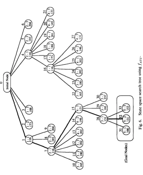
by node 4, which represents the partial assignment (2 - 1). The module M, has two immediate successors, M, and M4. The underestimate 103 is obtained by computing mu_x{min{l6 + 0 + 71+ 16, 16 + 27 + 88 + 16, 16 + 27+84+16), ml’n{16+0+86+16, 16+15+98+16, 16+15+24+16)]= mux{min{l03,147,143), min(ll8,145,71]} = max(l03,71]. Node 41 is a goal node, from which an optimal assignment (l-1,2-1,4-3,3-1,5-2> with minimal task turnaround time 131 is obtained. Only 43 search nodes are generated in Figure 5. Compared with 1788, which is the maximal number of nodes in the state space search tree, a saving of 1745 nodes is attained for this example.
The resulting state space search tree with respect to fATu is shown in Figure 6. In Figure 7, the computation of fATU(x) is illustrated by node 8, which represents the partial assignment (l-1,2-2). Processor turnaround
Fig. 6. State space search tree using faTo.
OPTIMAL ASSIGNMENT OF TASK MODULES 25 times for P,, P,, and P3 are 1, 89, and 0, respectively. There are three trauel pointers to nodes 4, 5, and 6 of the corresponding assignment tree shown in Figure 4. The underestimate 193 is obtained by computing mau(min{l + 99, 89 + 136, 1 + 144}, min(89 + 126, 89 + 104, 89 + 1391, min I89 + 141, 89 + 114, 89 + 77}} =max{lOO, 193,166). For this example, only 34 search nodes are generated, and a saving of 1754 nodes is attained. It can be observed from Figure 6 that for the example of Figure 2, at least 22 search nodes are generated in order to reach a goal node.
For the same example, 94 and 256 search nodes are generated, respec- tively, for Wang and Tsai’s algorithm and the A* algorithm with h(x) = 0.
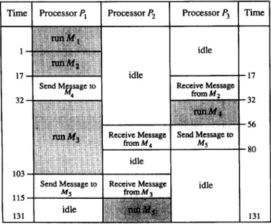
The schedule of the task execution with respect to the optimal assign- ment (l-1,2-1,4-3,3-1,5-2) is shown in Figure 8. The entire task termi- nates when M, is finished on processor P2.
4. EXPERIMENTAL RESULTS
In this section, we compare the performance of our algorithm with that of Wang and Tsai’s algorithm and the A* algorithm with h(x) = 0. The average number of search nodes, the maximal queue length of the unex- panded list, and the execution time are generated for performance evalua-
Time Processor PI Processor Pz Processor P3 Time
32 idle / idle I17 1 SendMRsageto 1 32 56 : 1 idle 1 idle I
Fig. 8. The schedule of the task execution with respect to the optimal assignment (l-1,2-1,4-3,3-1,5-2).
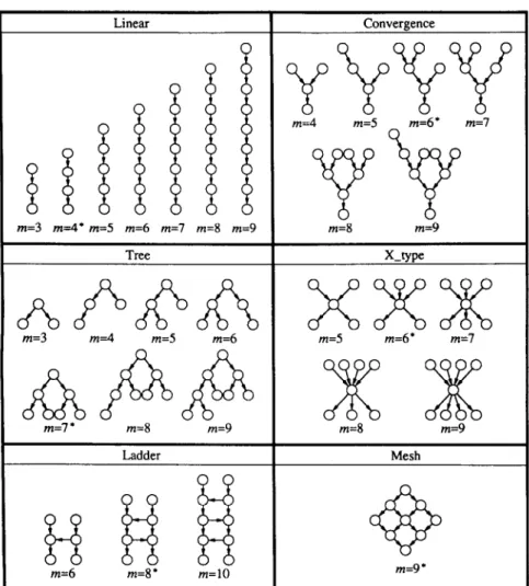
tion. In general, the performance of our algorithm is affected by many factors. Among them, four factors are considered in the experiment: the number of processors, the number of modules, the ratio of average intermodule communication time to average module execution time (called the C: P ratio), and the shapes of task graphs. The shapes of task graphs, which was neglected in [19], reflect the precedence relationship among all modules, and they will affect the accuracy of the estimation made by an underestimate function. In order to investigate the effect of the shapes of task graphs on the performance of our algorithm, instead of generating tested task graphs randomly, we consider six types of task graphs in the experiment: linear, convergence, X-type, tree, ladder, and mesh (see Figure 9).
A task graph is of the linear type if it forms a linear chain. In other words, if the precedence relationship among the modules is a total order then the corresponding task graph is of the linear type. A task whose execution consists of several serial phases has a linear-type task graph. A task graph is of the convergence type if it is a tree with the root downwards. A task has a convergence-type task graph it its modules can be partitioned into several disjoint subsets S,,S,,. ..,S, with ISrl>lS,l> a** a(S,I such that the precedence relationship only exists between Si and Si+ i, 1~ i Q r- 1. The tree-type tuskgruph is similar to the convergence-type task graph, except that the root of the tree is upwards. The X-type tusk graph and the mesh-type tuskgruph are two different combinations of the convergence-type task graph and the tree-type task graph. The ladder-type tuskgruph consists of two linear-type task graphs with some arcs between them. A task has a ladder-type task graph if its execution consists of two interreference execution paths.
A task graph with a look similar to one of these six types of task graphs is expected to have similar experimental results.
In our experiment, Wang and Tsai’s algorithm and the A* algorithm with h(x) = 0 are provided with the trivial initial solution (in [19], Wang and Tsai did not provide their algorithm with any initial solution). Addi- tional state space reduction rules that were introduced in the previous section are implemented in our algorithm. The intermodule communica- tion times are assumed uniform, that is, for two communicating modules M, and Mb, ZCT(u, b, i, j)‘s are the same for any i #j. Module execution times and intermodule communication times are generated randomly according to the given C : P ratios. The C : P ratios considered in our experiment are from 0.01 to 100 (or from - 2 to 2 using logarithmic values based 10).
In the rest of this section, experimental results about initial solutions and execution time are shown. For the sake of space, we do not show here
OPTIMAL ASSIGNMENT OF TASK MODULES 27 Linear Convergence *iijjI/ GYi$Y m=3 m=4'm=5 m=6 m=l m=8 m=9 m=8 m=9 Tree X-type AP&A xxx m=3 m=4 m=S m=6 m=5 m=6' m=7 iihh& x m=7* m=8 m=9 m=8 m=9 Ladder Mesh !-!RH j$? m=6 m=a * m=lO
Fig. 9. Six types of task graphs.
the experimental results about the average number of search nodes and the maximal queue length. Interested readers can find them in [20]. The experiment is carried out for different numbers of processors, different numbers of modules, different C : P ratios, and different types of task graphs. For each tested case, 200 randomly generated instances are run. Experimental results about initial solutions versus log,,JC: P> give the average values of 200 tested instances. Experimental results about execu- tion time versus log,,(C: PI give the total execution times of 200 tested instances.
In addition, experimental results about the average execution times versus the number of processors are shown. The average is taken with log,,(C : P) ranging from -2 to 2 (including 21 tested cases and 4200 tested instances in total). Experimental results about the average execu- tion time versus the number of modules can be found in [201.
4.1. INITLAL SOLUTIONS
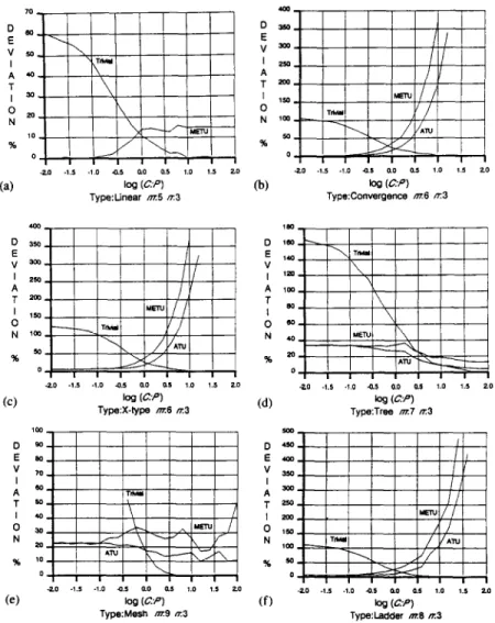
Figure 10 shows the deviation of initial solutions from the optimal solution as a function of log,,(C: P), where the curves labeled with “Trivial” represent the deviation of the trivial initial solution, and the curves labeled with “ATU” and “METU” represent the deviation of the two nontrivial initial solutions derived from the concepts of fATU and
f ,,,ETU,
respectively. It is seen that the trivial initial solution is very close to the optimal solution as log,,(C : P) > 0.5 for almost all types of task graphs (except tree-type task graphs). The performance of the two nontrivial initial solutions depends on not only the C : P ratios, but also the shapes of task graphs. In general, the nontrivial initial solutions are satisfactory when the intermodule communication time is less than the module execu- tion time, and they are almost optimal for linear-, convergence-, ladder-, and X-type task graphs. However, the nontrivial initial solutions have a great deviation when the intermodule communication time is greater than the module execution time. Fortunately, the trivial initial solution performs well in this case.Note that since the nontrivial initial solution derived from the concept of
fATu
is exactly an optimal solution to a linear-type task graph, any node expansion is unnecessary in this case. Therefore, experimental results with respect to the underestimate functionfATU
are not shown for the linear- type task graphs throughout this section.4.2. EXECUTION TIME
The number of search nodes and the maximal queue length are two important criteria for evaluating the performances of a BBU algorithm because they are machine independent and program independent. How- ever, they do not take the computational complexity of the underestimate function into consideration. A heavy computation of the underestimate on each search node may offset the gains from reducing the search space. Hence, the execution time is the most reliable measure to prove the effectiveness of a BBU algorithm. In our experiment, all of the tested
OPTIMAL ASSIGNMENT OF TASK MODULES 29 10
FM
cl E V Y) V I I A 40 A T T I 3o I 0 0 20 N N 10 % % (e)Fig. 10. Deviation of the initial solutions from the optimal solution versus log,,(C : P). Cd)
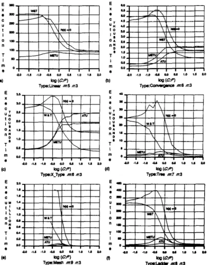
algorithms are programmed in C language to measure their execution times. The experimental results are shown in Figures 11-12.
Figure 11 shows the execution time of 200 randomly generated instances as a function of log,,(C : P> for our algorithm, Wang and Tsai’s algorithm, and the A* algorithm with h(x) = 0. The curves labeled with “ATU” and “METU” represent the results of our algorithm using the underestimate functions fATU and
fMETu,
respectively. The curves labeled with “W&T”Fig. 11. Execution time of 200 tested instances versus log,,(C: P).
and “h(x) = 0” represent the results of Wang and Tsai’s algorithm and the A* algorithm with h(x) = 0, respectively. It is seen that our algorithm and
Wang and Tsai’s algorithm are opposite in performance.
It can be observed from Figure 11(a) that our algorithm performs better than the other two algorithms everywhere for the linear-type task graph of m = 5. Wang and Tsai’s algorithm has a bad performance, even worse than the A* algorithm with h(x) = 0, as log,,(C : P) < - 0.8. This is due to the potential weakness of their algorithm in estimating the minimal task turnaround time for a “slim” and “long” task graph. Also note that the
OPTIMAL ASSIGNMENT OF TASK MODULES 31 Numbu d Pro==-(n) TypeLinear m.5 m b (dl
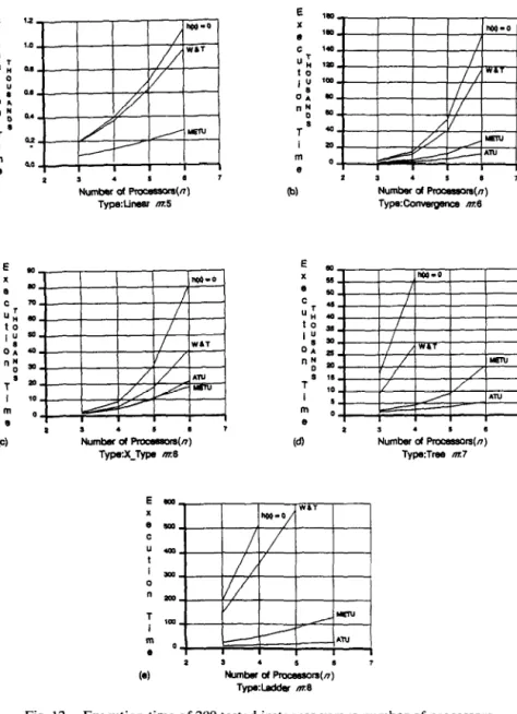
Fig. 12. Execution time of 200 tested instances versus number of processors.
curve labeled with “W&T” drops drastically as the C: P ratio > -0.8, which is mainly due to the high accuracy of the trivial initial solution as the C: P ratio is high, and not Wang and Tsai’s algorithm itself.
Figure 11(b) shows experimental results for the convergence-type task graph of m = 6. The curve labeled with “W&T” is higher than the curve
labeled with ‘%(x)=0” as log,,(C: P) < - 1. Our algorithm performs better than the other two algorithms as log,,(C : P) < 0.2. As log,,(C : P) > 0.5, Wang and Tsai’s algorithm has the best performance.
Figure 11(c) shows experimental results for the X-type task graph of m = 6. Our algorithm performs worst for the X-type task graph among all six types of task graphs. Even so, our algorithm has a satisfactory pe~o~ance as log,,fC : P> < 0.
Figures 11(d)-(f) show experimental results for tree-, mesh-, and ladder-type task graphs, respectively. The reason for the ruggedness of Figure 11(d) is the random generation of tested instances in our experi- ment, Because of strict memory limitations in the experimental environ- ments, Figure 11(e) shows only partial curves of “h(x) = 0” and “W&T.” Our algorithm performs well for these three types of task graphs. More- over, it can be found that for all six types of task graphs but the X-type, the performance of our algorithm is stable for all C : P ratios.
Figure 12 shows the execution time of 200 test instances for different numbers of processors. For each tested case, the result is obtained by taking an average on all log,,(C: P) values from - 2 to 2. Our algo- rithm has a better performance than Wang and Tsai’s algorithm in all tested cases. Because of memory limitations, experimental results for the mesh-type task graph are not shown here.
Interested readers can find in 1201 experimental results about the aver- age execution time versus the number of modules. Like Figure 12, the average is taken with log,,(C :P) ranging from - 2 to 2. Our algorithm has a better performance than Wang and Tsai’s algorithm almost everywhere.
5. CONCLUDING REMARKS
In this paper, we have proposed a BBU algo~thm for the task assign- ment problem, which was considered by Wang and Tsai [19]. The essence of Wang and Tsai’s algorithm is to underestimate the minimal task tu~around time from the vie~oint of a bottleneck processor, This causes their algorithm to be a poor underestimation as the C: P ratio is low. On the other hand, our algorithm underestimates the minimal task turnaround time from the viewpoint of execution paths. E~erimental results provide us with a complete comparison among our algorithm, Wang and Tsai’s algorithm, and the A* algorithm with h(x) = 0. Our algorithm is stable in performance and has the best performance in most tested cases. Wang and Tsai’s algorithm degenerates rapidly as the C : P ratio decreases, and its instability in performance makes it less attractive in practical applications. The A* algorithm with h(x) = 0 acts as a benchmark (upper bound) for the BBU algorithm.
OPTIMAL ASSIGNMENT OF TASK MODULES 33 In order to investigate the effect of the shapes of task graphs on the performance of our algorithm, we consider six types of task graphs: linear, convergence, X-type, tree, ladder, and mesh in the experiment. Experimental results show that our algorithm is the most favorable to the execution of linear-type task graphs, but has a worse execution of X-type task graphs as the C: P ratio is high. Our algorithm, using the underesti- mate function fATU, can obtain an optimal solution to a linear-type task graph without any node expansion.
A good initial solution can fathom many search nodes at the beginning of state space search. In our experiment, each of the tested algorithms is provided with an initial solution (no initial solution is suggested in [19] for Wang and Tsai’s algorithm). The trivial initial solution is almost an optimal solution as log,,(C : P) > 0.5 for linear-, convergence, X-type-, mesh-, and ladder-type task graphs. On the other hand, nontrivial initial solutions are almost an optimal solution as log(C : P) < - 0.5 for linear-, convergence-, X-type, and ladder-type task graphs. Moreover, the nontrivial initial solution using the concept of fATu is exactly an optimal solution to a linear-type task graph.
In addition, some state space reduction rules were introduced to further reduce the search space. According to these rules, constraints may be generated during state space search for a search node. These constraints can cause more search nodes fathomed during execution.
The authors are pleased to thank the anonymous referees for their valuable suggestions and comments.
REFERENCES
1. S. H. Bokhari, Dual processors scheduling with dynamic reassignment, IEEE Transactions on Software Engineering SE-5(4):341-349 (1979).
2. S. H. Bokhari, A shortest tree algorithm for optimal assignments across space and time in a distributed processor systems, IEEE Transactions on Sofhvare Engineering SE-7(6):583-589 (1981).
3. S. H. Bokhari, On the mapping problem, IEEE Transactions on Computers C-30(3):207-214 (1987).
4. S. H. Bokhari, Partitioning problems in parallel, pipelined, and distributed comput- ing, IEEE Transactions on Computers C-37(1):48-57 (1988).
5. M. S. Chern, G. H. Chen, and P. Liu, An LC branch-and-bound algorithm for module assignment problem, Information Processing Letters 32(2):61-71 (1989). 6. K. Efe, Heuristic models of task assignment scheduling in distributed systems, IEEE
Computer 15:50-56 (1982).
7. E. Horowitz and S. Sahni, Fundamentals of Data Structures, Computer Science Press, Rockville, MD, 1976.