以去背相連性為基礎之立體匹配研究

(1)

國立交通大學

電子工程學系電子研究所碩士班

碩

士

論

文

以去背相連性為基礎之立體匹配研究

A Study on

Matting Affinity Based Stereo Matching

研

究

生：宋秉修

指導教授：王聖智教授

簡鳳村教授

(2)

以去背相連性為基礎之立體匹配研究

A Study on

Matting Affinity Based Stereo Matching

研究生：宋秉修 Student：Bing-Shiou Sung

指導教授：王聖智教授 Advisor：Prof. Sheng-Jyh Wang

指導教授：簡鳳村教授 Advisor：Prof. Feng-Tsun Chien

國立交通大學

電子工程學系電子研究所碩士班

碩士論文

A Thesis

Submitted to Department of Electronics Engineering & Institute of Electronics College of Electrical and Computer Engineering

National Chiao Tung University in partial Fulfillment of the Requirements

for the Degree of Master of Science in

Electronics Engineering

September 2012

Hsinchu, Taiwan, Republic of China

(3)

以去背相連性為基礎之立體匹配研究

研究生：宋秉修

指導教授：王聖智教授

指導教授：簡鳳村教授

國立交通大學

電子工程學系電子研究所碩士班

摘要

基於一些技術方面的需求，立體匹配已成為一個討論很久的議題而且現今也有許多既有的演算法，這些演算法大致上可以分成兩種種類：局部演算法和整體演算法，而每一類的演算法都有他們獨特的優缺點。其中，整體演算法不但能實現整體演算法的結果，整體演算法也可以採用一些實現局部演算法的方法。所以在我們的論文中採用了整體演算法的架構去建立一個系統來解立體匹配的問題，而這個系統同時能達到局部演算法跟整體演算法的優點。另一方面，我們也從影像去背的影像處理議題中引進了一個叫做去背相連性的函數到我們的整體演算法中，使我們希望能夠透過使用這個函數，只需要用到整體演算中常用到的兩個計算費用函數的項：資料項和平滑項，就可以達到跟一些現有的論文中外加了許多費用函數項一樣的結果。

(4)

A Study on

Matting Affinity Based Stereo Matching

Student：Bing-Shiou Sung Advisor：Prof. Sheng-Jyh Wang

Advisor：Prof. Feng-Tsun Chien

Department of Electronics Engineering, Institute of Electronics

National Chiao Tung University

Abstract

Stereo matching has been a long discussed issue for some technological needs, like 3D scene reconstruction. A large number of algorithms for stereo matching have been developed. Most of the algorithms can be categorized into two types: local and global algorithms. Each category has its own pros and cons. However, global algorithms can not only do the work of global algorithms but also can adopt some methods used in local algorithms, like cost aggregation. Therefore in this thesis, we construct a system based on a global-type algorithm to leverage between the advantages of both local and global algorithms. In addition, we introduce the matting affinity function which comes from image matting processing into the global algorithms of stereo matching in order to achieve a better result by using only traditional term costs: the data term cost and the smoothness term cost.

(5)

致謝

在此特別感謝指導教授王聖智老師，在這兩年的碩士生涯中給予的許多教導與建議，包含人生經驗的分享、求學經驗的心得、研究和念書的精神與態度以及做人處事的道理，老師的教誨有如時雨春風令我獲益良多，面對未來的挑戰時，希望能將老師的教導謹記在心。同時也要感謝全體實驗室夥伴的扶持與陪伴，包含博士班學長：禎宇、家豪，碩士班學長：奕安、維辰、玉書、韋弘、鄭綱、郁霖、開暘，同屆的同學：心憫、彥廷、耀笙、柏翔，碩士班學弟妹：姿婷、秉宸、政銘、介暐、佳峻、家駿，無論是學業或研究上的討論以及一起運動、聚餐，都讓我這兩年的研究生活過得充實且愉快。很榮幸成為 Vision Lab 的一員，希望未來還有機會和大家保持聯絡、互相幫助。

(6)

Content

CHAPTER 1 . INTRODUCTION... 1 CHAPTER 2 . BACKGROUNDS ... 5 2.1SIMILARITY MEASURES ... 6 2.2LOCAL ALGORITHMS ... 8 2.3GLOBAL ALGORITHMS ... 11

2.4MATTING AFFINITY FUNCTION ... 13

CHAPTER 3 . PROPOSED METHOD ... 17

3.1PROPOSED GLOBAL ALGORITHM FOR STEREO MATCHING... 18

3.2PROPOSED METHOD FOR SOLVING GLOBAL OPTIMIZATION ... 21

3.3PROPOSED SYSTEM ... 23

CHAPTER 4 EXPERIMENTAL RESULTS ... 29

CHAPTER 5 CONCLUSION ... 46

(7)

List of Figures

Figure 1-1 An illustrative example of the disparity. ... 1

Figure 1-2 Epipolar line: a pixel in an image may be a line segment in another image. ... 2

Figure 1-3 Images are made to be rectified image to simplify matching process in stereo matching. ... 3

Figure 1-4 Inputs and output of stereo matching. ... 4

Figure 2-1 Pixels with no specific textures are hard to find their matching pixels. ... 5

Figure 2-2 Pixels are occluded by the foreground object. ... 6

Figure 2-3 Matching process takes care of all the possible disparities and then assigns the one with the minimum difference. ... 7

Figure 2-4 Window-based method. ... 7

Figure 2-5 Problem for traditional window-based method occurs at the edge. ... 8

Figure 2-6 Adaptive window method. ... 9

Figure 2-7 Criterion: left/right consistency checking. ... 10

Figure 2-8 Connection weight between pixels. ... 11

Figure 2-9 Input and output of image matting. ... 13

Figure 2-10 Inputs and output of supervised matting. ... 14

Figure 2-11 Matting affinity function takes the information of all the pixels inside a window into consideration. ... 16

Figure 3-1 Local algorithms are good at preserving the values of disparity over small regions in the image. ... 17

Figure 3-2 Global algorithms are good at generating a smoother disparity map. ... 18

Figure 3-3 Maps of “pixel with inconsistent disparity (PID)”. Inconsistent parts are indicated in white. ... 20

Figure 3-4 Confidence map: white for high confidence and black for low confidence. ... 23

Figure 3-5 Proposed system block diagram. ... 24

Figure 3-6 Small regions may get merged into neighboring regions if the smoothness term is considered. ... 25

Figure 3-7 Textureless region may get merged into the nearby region if the smoothness term is considered. ... 25

(8)

Figure 3-9 System Process in detail. ... 28 Figure 4-1 Test patterns: (a) Tsukuba pair, (b) Venus pair, (c) Teddy pair, (d)

Cones pair. ... 30 Figure 4-2 Ground truths: (a) Tsukuba ground truth, (b) Venus ground truth, (c) Teddy ground truth, (d) Cones ground truth. ... 31 Figure 4-3 Outputs of the first system block: (a) initial disparity map of left

image, (b) initial disparity map of right image, (c) confidence map of left image, (d) confidence map of right image. ... 32 Figure 4-4 Outputs of second system block: (a) disparity map of left image,

(b) disparity map of right map, (c) confidence map of left image, (d) confidence map of right map, (e) PID map of left image, (f) PID map of right map. ... 33 Figure 4-5 Outputs of the third system block: (a) disparity map of left image,

(b) disparity map of right image. ... 34 Figure 4-6 Tsukuba: (a) disparity map of our method, (b) ground truth. .... 34 Figure 4-7 Outputs of the first system block: (a) initial disparity map of left

(b) disparity map of right map, (c) confidence map of left image, (d) confidence map of right map, (e) PID map of left image, (f) PID map of right map. ... 36 Figure 4-9 Outputs of the third system block: (a) disparity map of left image,

(b) disparity map of right image. ... 37 Figure 4-10 Venus: (a) disparity map of our method, (b) ground truth. ... 37 Figure 4-11 Outputs of the first system block: (a) initial disparity map of left

(b) disparity map of right map, (c) confidence map of left image, (d) confidence map of right map, (e) PID map of left image, (f) PID map of right map. ... 39 Figure 4-13 Outputs of the third system block: (a) disparity map of left

image, (b) disparity map of right image. ... 40 Figure 4-14 Teddy: (a) disparity map of our method, (b) ground truth. ... 40 Figure 4-15 Outputs of the first system block: (a) initial disparity map of left

image, (b) initial disparity map of right image, (c) confidence map of left image, (d) confidence map of right image. ... 41

(9)

Figure 4-16 Outputs of second system block: (a) disparity map of left image, (b) disparity map of right map, (c) confidence map of left image, (d) confidence map of right map, (e) PID map of left image, (f) PID map of right map. ... 42 Figure 4-17 Outputs of the third system block: (a) disparity map of left

image, (b) disparity map of right image. ... 42 Figure 4-18 Cones: (a) disparity map of our method, (b) ground truth. ... 43

(10)

List of Tables

Table 4-1 Results of Tsukuba on Middlebury ... 44

Table 4-2 Results of Venus on Middlebury ... 44

Table 4-3 Results of Teddy on Middlebury ... 45

(11)

Chapter 1. Introduction

For technological needs, like 3D scene reconstruction, it has been a long discussed issue about how to find the depth information of a 3D scene by image or video. Stereo matching, which imitates the human vision to get the depth information, is one of the discussed solutions.

How does stereo matching do to get the depth information? From the earliest inquiries into visual perception, it was known that we perceive depth based on the differences in appearance between the left and right eye. It means that one specific point in the vision of left eye appears in the vision of right eye with a different coordinate as shown in Figure 1-1. The amount of this difference, so-called “disparity” in stereo matching, is inversely proportional to the distance from the observer. By computing these disparities, we’ll get the depth information of the 3D scene.

(12)

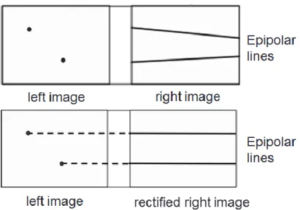
Before we compute the disparity, we need to find the matching pixel in the right image for each pixel in the left image. To speed up the matching process and increase its reliability, we only need to find the matching point in a certain range instead of the whole image. The certain range is so-called the epipolar line. Figure 1-2 shows how a pixel XL in one image projects to an epipolar line segment in the other image.

The epipolar line can be computed by intrinsic camera parameters which are already known. However, to simplify the matching process, the images are made to be rectified images. It means that the corresponding epipolar lines are just horizontal scan lines as shown in Figure 1-3. That is, the right image is just the left image with a horizontal shift.

Figure 1-2 Epipolar line: a pixel in an image may be a line segment in another image.

To sum up, stereo matching is the process of taking two images and estimating the depth of the scene by ﬁnding matching pixels in the two images. The inputs are two images and the output is the “disparity map” as shown in Figure 1-4.

(13)

Figure 1-3 Images are made to be rectified image to simplify matching process in stereo matching.

Many algorithms have been developed in the literature for stereo matching. All the algorithms can be categorized into two categories: local and global algorithms. Each category has its own pros and cons. The main contribution of this research is that we propose a global algorithm that not only preserve the advantages of both local and global algorithms, but also incorporate the idea of “matting affinity function” into global algorithms that leads to performance improvement in the stereo matching result.

The rest of the thesis is summarized as follows. In Chapter 2, we will summarize the backgrounds of the local and global algorithms. Also, the matting affinity function will be explained in details in this chapter. In Chapter 3, we will present our proposed method and system. Experimental results will be shown in Chapter 4. Finally, we will give our conclusion in Chapter 5.

(14)

(15)

Chapter 2. Backgrounds

Stereo matching is an issue which has been discussed for a long time. Many algorithms have been developed to solving stereo matching. There has been a website [1] for discussing the issues of stereo matching. Lots of problems, such as the edge-preserved issue and edge-fatten problem, have been solved in [3]. However, there are still challenges for stereo matching. “Matching for textureless pixels” and “refining disparity of occluded pixels” are two main challenges for stereo matching. The former shows the problem that it’s hard to find the matching pixels in the corresponding image for the pixels with no specific textures, because of the presence of multiple matching candidates as shown in Figure 2-1. On the other hand, the latter shows the problem that the occluded pixels are difficult to find their matching pixels in the corresponding image because the actual matching pixels can’t be seen in the corresponding image as shown in Figure 2-2.

(16)

Figure 2-2 Pixels are occluded by the foreground object.

All the algorithms developed to solve stereo matching problem can be categorized into two categories: local and global algorithms. Local algorithms compute the disparity pixel by pixel and focus on designing an adaptive window and refining the pixels with wrong disparities. On the other hand, global algorithms decide the disparity altogether after gathering all the information of the whole image and focus on defining a global cost function and solving global optimization problem. More details will be introduced in the following sections.

2.1 Similarity Measures

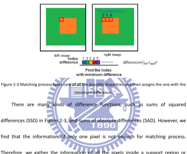
Before introducing algorithms, we first introduce the similarity measures. In the matching process, we have to check the similarity of colors, intensities, gradients…etc. between pixels. To check the similarity, we usually define a function called difference function. If the value of the difference function is low, the similarity between pixels is high, indicating that the pixel may be the matching pixel we want to find. The traditional matching process is shown in Figure 2-3. Traditional matching process

(17)

computes the difference values of all the possible disparities and saves them in a vector. We find the disparity with the minimum difference from the vector and assign it into the pixel.

Figure 2-3 Matching process takes care of all the possible disparities and then assigns the one with the minimum difference.

There are many kinds of difference functions, such as sums of squared differences (SSD) in Figure 2-3, and sums of absolute differences (SAD). However, we find that the information of only one pixel is not enough for matching process. Therefore, we gather the information of all the pixels inside a support region or window that is centered on the pixel where we want to assign the disparity as shown in Figure 2-4. This is the so-called window-based method.

(18)

2.2 Local Algorithms

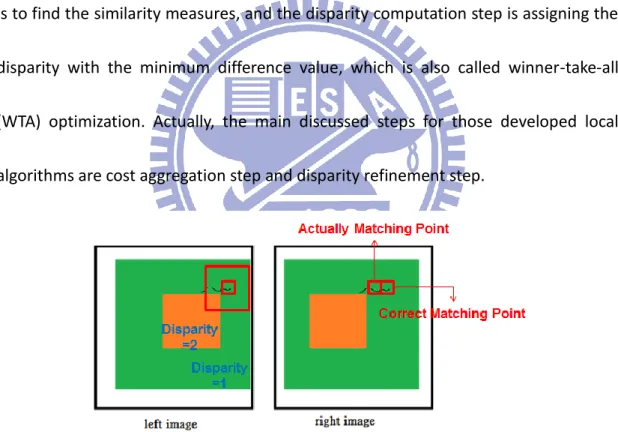
Local algorithms are based on the window-based method. As mentioned previously, local algorithms compute the disparity pixel by pixel, and the detail for its matching process is just as the traditional one. R. Szeliski [2] summarized four main steps for the local algorithm: matching cost computation, cost aggregation, disparity computation, and disparity refinement. The goal of matching cost computation step is to find the similarity measures, and the disparity computation step is assigning the disparity with the minimum difference value, which is also called winner-take-all (WTA) optimization. Actually, the main discussed steps for those developed local algorithms are cost aggregation step and disparity refinement step.

Figure 2-5 Problem for traditional window-based method occurs at the edge.

The cost aggregation step is to gather the information, or to sum the difference values, of all the pixels inside the support window. However, there is a big problem that might possibly occur in the window-based method, as illustrated in Figure 2-5. If we use the traditional window-based method, we will obtain a wrong disparity at the

(19)

pixel outside the edge of a foreground object. This problem is called the edge-fatten problem. This problem occurs because we take the information of pixels which are not located on the same object as the pixel that we are supposed to assign disparity to.

To tackle this problem, an adaptive window method was developed in [3]. The adaptive window method says that we only have to take the information of the pixels which are located on the same object as the pixel that we are supposed to assign disparity to. The way to achieve this method is to add a term called the weight function as shown in Figure 2-6. It means that if this pixel is similar to the centered pixel, then we’ll take it into consideration; while if this pixel is different from the centered pixel, we won’t take its information. The following local algorithms are based on the adaptive window method and find new way to improve it. For example, Zhang et al. [5] designed a non-squared region for the adaptive window. This is called the cross-based aggregation method.

(20)

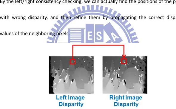
Another commonly discussed step is the disparity refinement step. This step aims to find the pixels with wrong disparities and refine them. Bleyer et al. [6] defined a criterion by checking the two disparity values of the two matched pixels in the left and right images. A pixel in the left image can find its corresponding pixel in the right image by its disparity. The corresponding pixels should have the same disparity. This criterion is called left/right consistency checking as shown in Figure2-7. By the left/right consistency checking, we can actually find the positions of the pixels with wrong disparity, and then refine them by propagating the correct disparity values of the neighboring pixels.

Figure 2-7 Criterion: left/right consistency checking.

The challenges for stereo matching are taken into consideration in the above two steps to achieve different solutions in different research works. The advantages of local algorithms are low computational time and having detailed disparity.

(21)

2.3 Global Algorithms

Global algorithms show another way to solve stereo matching problem. Instead of deciding disparity pixel by pixel, global algorithms say that the pixels located on the same object should have the same or close disparity value. Therefore, they should have to decide their disparity at the same time. In addition to computing the different values of all possible disparity of all the pixels as is done by the local algorithms, global algorithms also compute the similarity between the pixel and the neighboring pixels to achieve the statement above. This similarity is called the connection weight in global algorithms as shown in Figure 2-8. If the similarity between pixels is high, they should have the same or close disparity. If they don’t, to achieve the statement above, we’ll give them a penalty, called the label cost, in order to prevent the situation that similar pixels result in noticeable different values of disparity.

(22)

To sum up, global algorithms first compute the difference values which are called the data term costs Ci in global algorithm. The sum of the penalties for similar

pixels with different values of disparity is called the smoothness term costs (2.1). Finally, we can write the total global cost function as (2.3) and try to find the solution for disparity that minimizes the total cost. This is the so-called global optimization problem. The main steps of the global algorithms are to define a new global cost function and to find a proper global optimiztion algorithm to solve it.

Smoothness term:

∑ W

∗ P

(2.1)

W

: the connection weight between pixel i and j:

P

: penalty for similar pixels I and j with different values of disparity

P

= constant or (d

− d

)

2

(2.2)

d

: the disparity value of pixel i

d

: the disparity value of pixel j

Total cost function:

E(disparity)=∑ (C

+ ∑ W

∗ P

)

(2.3) Data term cost:

C

In addition to the data term and smoothness term costs, some theses add other term costs into the global cost function in order to solve some problems. For example, Z. Wang [9] added the occlusion term cost to solve the occlusion problem, and M. Bleyer [10] added the soft segmentation term, curvature term, and minimum

(23)

description length (MDL) term costs.

Many global optimization algorithms have been proposed to solve the global stereo matching problem, such as the graph cut and belief propagation. Although these algorithms can only get the local minimum solution, they still perform very well on solving the global stereo matching problem. The advatages of global algorithms include having only one stage to get the solution and having smooth results of disparity. However, the computational time of global algorithms is much higher than that of the local algorithms.

2.4 Matting Affinity Function

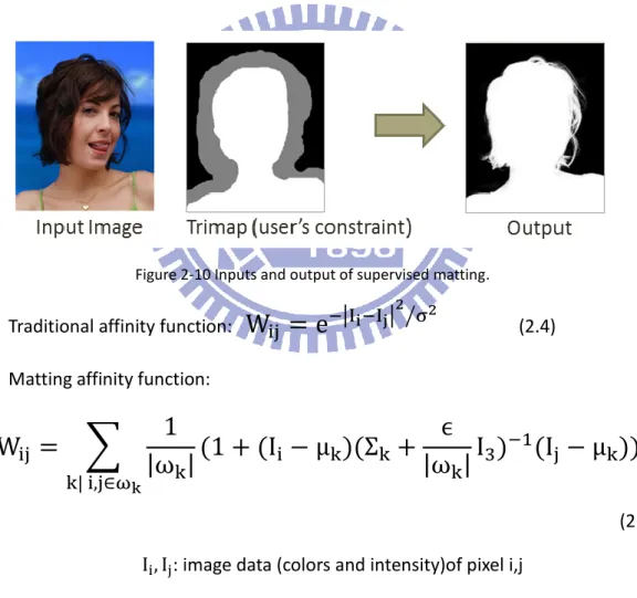
Matting affinity function comes from another issue of image processing called image matting. Image matting is an image processing technique that attempts to extract a foreground object from an image along with an opacity estimate for each pixel covered by the object, as shown in Figure 2-9. The problems of Image matting can be divided into two categories: supervised matting and unsupervised matting.

(24)

The affinity function is first used in supervised matting. The input of supervised matting is not only the input image but also the map with some known results, as shown in Figure 2-10. This map, called the trimap, has the results of some pixels. For example in Figure 2-10, the black part of the trimap is already known as background, and the white part of the trimap is known as the foreground object. Supervised matting tries to find an algorithm to train the result of the gray part of the trimap.

Figure 2-10 Inputs and output of supervised matting.

Traditional affinity function:

W

= e

| | ⁄ (2.4) Matting affinity function:

W

= ∑

1 |ω

_k

|

(1 + (I

− μ

k

)(Σ

k

+

ϵ

|ω

_k

|

I

3

)

1

(I

− μ

k

))

k| , ∈ω_k (2.5) I, I: image data (colors and intensity)of pixel i,j

ωk: support window

μ_k: mean value of the image data of pixels inside the support window Σk: variance of the image data of pixels inside the support window

(25)

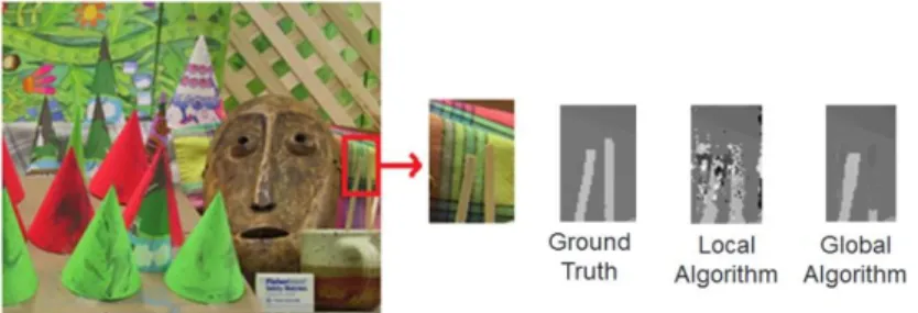
This means that supervised matting has to infer the result of the gray part of the trimap by the information of input image and known results. To achieve this goal, we first have to obtain the relationship between pixels, and then refine the pixels of the gray part by the results of the known pixels with close relationship. The function for computing the relationship is the so-called affinity function. Equation (2.4) shows the traditional affinity function which is the same as the connection weight function of the global algorithms for stereo matching. Levin et al. [7] achieved a better result in image matting processing by using a new method and redefining the affinity function, called the matting affinity function as shown in (2.5).

The matting affinity function can achieve a better result for computing relationship between two pixels because the function considers the information of all the nearby pixels inside a fixed window as shown in Figure 2-11 instead of considering only the information of the two pixels. In the equation (2.5), |ωk| is the

size of the support window. Ii and Ij are the color information (red, green, blue) of the

two pixels. μk is the average color values of the pixels inside the support window and

Σk is the covariance matrix for the pixels inside the support window. I3 is an identity

matrix and 𝛜 is a constant coefficient.

For the reasons that the affinity function in image matting is defined the same as the connection weight function in stereo matching and that matting affinity

(26)

function achieved better results in image matting, we attempt to employ the matting affinity function into the proposed global algorithm for stereo matching in order to improve the results of stereo matching.

Figure 2-11 Matting affinity function takes the information of all the pixels inside a window into consideration.

(27)

Chapter 3. Proposed Method

In the previous chapter, we have mentioned the two main challenges for stereo matching and have introduced the underlying operations for both local and global algorithms. Each algorithm has its advantages. Local algorithms are good at preserving the values of disparity over small regions in the image, as shown in Figure 3-1 because the disparity value is assigned pixel by pixel. On the other hand, global algorithms may sometimes mistakenly merge small region into a neighboring bigger region whose disparity value is actually different from the disparity value of the small region. In this case, the small region will be assigned an incorrect disparity value. However, global algorithms are good at generating a smoother disparity map as shown in Figure 3-2 because of the inclusion of a smoothness term in the cost function. In comparison, local algorithms usually generate rugged disparity map. If we can take the advantages of both local and global algorithms, a more accurate estimation of the disparity map can be expected.

Figure 3-1 Local algorithms are good at preserving the values of disparity over small regions in the image.

(28)

Figure 3-2 Global algorithms are good at generating a smoother disparity map.

How can we take the advantages of both local and global algorithms? Actually, given a global algorithm, if we remove the prior term from the cost function and consider the data term over each local region, this global algorithm will be reduced to a local algorithm. This means that we can partially incorporate methods used in the local algorithms into the global algorithms. This is the main reason why we choose global algorithms in our thesis. In the following sections, we will introduce our proposed global algorithm, the method that we solve global optimization problem, and the structure of our system.

3.1 Proposed Global Algorithm for Stereo Matching

In this section, we will discuss the proposed global cost function. In the next section, we will discuss the method used to solve the global optimization problem. Recent global algorithms usually introduce extra terms in the global cost function in order to improve the result of the estimated disparity map. In our method, we only use the data term and smoothness term, but with new definitions.

(29)

E

(d

) =

∑ _∈ ∑_∈W[(I( ) − I( − d)) ] (1 − φ( )) + α ∗ φ( ) (3.1)

Weight function:

W

= e

| | ⁄ (3.2)

Pixel with inconsistent disparity (PID):

φ

= {

1 f d

( − d

( ))

≠ d

( )

0 otherw se

(3.3)

The proposed data term, the first component in (3.1), computes the sum of squared differences (SSD) over an adaptive window, as mentioned in Chap. 2. The reason for using the adaptive window based cost aggregation is to adopt the advantage of the local algorithm in the proposed algorithm. In (3.1), Wij is the weight

function for computing the similarity between pixels. The size N of the adaptive window is defined as an adjustable parameter, since we would like to pay attention to refining the pixels with wrong disparity in some blocks of our proposed system. In this case, we need more information to do so. The detail will be introduced in section 3.3. And then, we try to consider the effect of the occlusion problem into the data term cost. The concept is that the pixels occluded by the foreground object are not supposed to find its matching pixels by data term cost and their disparity values should be refined by the neighboring pixels with correct disparity. Therefore, if the

(30)

pixel is occluded or checked to have wrong disparity, we should block the decision of the data term, and refine the real value of disparity by the smoothness term. This work is done by the proposed “Pixel with inconsistent disparity (PID)” which uses the criterion based on left/right consistency checking in [6]. The disparity value of a pixel in the left image should be the same as the disparity value of its matching pixel in the right image. If a pixel is checked to be with inconsistent disparity, the PID of this pixel is set to 1 as shown in (3.3) and Figure 3-3, and then the data term cost will be set to be a constant value α.

The proposed smoothness term replaces the traditional connection weight function by the matting affinity function as shown in (3.4). As mentioned previously, we have to give a penalty for similar pixels with different values of disparity. The penalty is defined as the squared difference of the values of disparity as shown in (3.5).

(31)

Connection weight function = matting affinity function:

W

= ∑

1 |ω

_k

|

(1 + (I

− μ

k

)(Σ

k

+

ϵ

|ω

_k

|

I

3

)

1

(I

− μ

k

))

k| , ∈ω_k (3.4)

Penalty

= (d

− d

)

(3.5)

E

(d

) = ∑

W

( , ) ∗ (d

− d

)

(3.6)

Therefore, our proposed total global cost function is summarized as follows. β is an adjustable scalar for the smoothness term.

E

(d

) =

∑ ∑

e

−|I−I|2⁄ 2[(I( ) − I( − d)) ] (1 − φ( )) + α ∗ φ( ) ∈

+β ∗ ∑

W

∗ (d

− d

)

(3.7)

3.2 Proposed Method for Solving Global Optimization

As mentioned previously, there are already many available algorithms for solving global optimization problem. However, these algorithms may not be able to find the global optimum solution unless the global cost function can be defined as a closed-form formulation. This is the reason why we use the squared form to define

(32)

our cost function.

Nevertheless, although the closed-form formulation of our proposed global cost function has been derived, we still have difficulty accomplishing it. Hence, we choose another method to get the same solution as a closed-form solution. First, we adopt an available algorithm: GCoptimization, which is a software work for energy minimization with graph cuts [12]. This algorithm provides codes for solving multi-labeling problem with graph cuts algorithm. In the first module of our system which will be introduced in Section 3.3, we only this software to get the initial values of the disparity map.

In other system modules, before computing the disparity map by the GCoptimization software, we have another stage for refining the disparity map. This stage is to prevent from getting a local optimum solution. In this stage, a maximum-a-posterior (MAP) estimation problem based on [8] is solved. The concept of this stage is that if we know the confidence of the input result, we can refine these pixels with inconsistent disparity based on the disparity information of the pixels with higher confidence. The estimation problem is expressed in Equation (3.8). Here, we have the input y and its confidence map Λ. The confidence map is obtained also by the left/right consistency check. That is, if the PID of a pixel is set to be 1, then the confidence value of the pixel is set to be 0, as shown in Figure 3-4. L is called the

(33)

matting laplacian matrix and can be seen as another expression of the aforementioned matting affinity function. The last term of Equation (3.8) does the same work as the smoothness term in the global optimization problem.

We have to estimate the final result d by minimizing the cost function in (3.8). Because this cost function is defined as a closed-form formulation, the global minimum of (3.8) can be obtained by solving the linear equation in (3.9).

Estimation problem

:

E(d) = (d − y)

Λ(d − y) + d

Ld

(3.8)

d

Ld =

1

∑ w

_,

(d

− d

)

w :matting affinity function

(L + Λ)d = Λy

(3.9)

Figure 3-4 Confidence map: white for high confidence and black for low confidence.

3.3 Proposed System

In our proposed system, there are three main system blocks as shown in Figure 3-5. In each block, there are three common processes: defining the total cost function, solving it by our proposed method, and checking left/right consistency. Each block is designed for different purposes and the details will be introduced later.

(34)

Figure 3-5 Proposed system block diagram.

Before introducing the details of each block, we summarize all the adjustable parameters first. The adaptive square window size N is to adjust the influence of cost aggregation in each block. The scalar β for the smoothness term is to adjust the influence of the smoothness term. The parameter T denotes the number of iterations in the system block.

In the first system block shown in Figure 3-5, we try to save the detailed result computed by the cost aggregation only. The reason we do not consider the smoothness term is to avoid merging small regions into their neighboring regions at this stage. For the example shown in Figure 3-6, the foreground chopsticks whose disparity value is actually different from that of the background may get merged into the background region if smoothness constraint is included at this stage. Another example is shown in Figure 3-7 in which the white background region which is

(35)

basically textureless will also get merged into the nearby chimney region if the smoothness constraint is considered.

Figure 3-6 Small regions may get merged into neighboring regions if the smoothness term is considered.

Figure 3-7 Textureless region may get merged into the nearby region if the smoothness term is considered.

Based on the above discussion, we assign a big enough size N for the adaptive window and a scalar β for the smoothness term. On the other hand, this system block has no initial disparity map. Hence, we solve this system block only by using the GCoptimization software with the graph cut algorithm.

The second system block shown in Figure 3-5 is designed to refine the result computed by the first system block with a large β for the smoothness term but without the use of PID. The reason not to use PID is that we don’t handle the

(36)

occlusion problem in this system block but only focus on refining the disparity values of the textureless regions instead. If we include PID at this stage, textureless regions will be treated as occluded regions and will not be assigned the correct disparity value. As mentioned previously, for textureless pixels, it is hard to find their matching pixels because of the existence of multiple candidates. This situation is not the same as that of occlusion problem. Therefore, these two conditions should be treated differently. In our system, we consider both cost aggregation and smoothness term at this stage and leave the occlusion problem to the third system block. Hence, we set the same window size N as that in the first system block while a bigger β to increase the influence of the smoothness term. On the other hand, this system block has the initial disparity map. Hence, in this system block, we use a matting laplacian based estimation, together with the GCoptimization software with the graph cut algorithm.

Figure 3-8 The light brown region has the textureless problem.

The third system block shown in Figure 3-5 is designed to focus on solving the occlusion problem. As mentioned previously, for the occluded pixels, we cannot find

(37)

their matching pixels in the corresponding image. All we can do is to find the locations of these occluded pixels and to refine their disparity value by nearby pixels that have the correct disparity value. In this system block, the smoothness term becomes more important. On the contrary, the cost aggregation term is no longer important. Hence, in this system block, we do not use the cost aggregation term or just set the window size N to 1. We also assign a large β for smoothness term to refine pixels with inconsistent disparity values. Since this system block also has the initial disparity map. We use the matting laplacian based estimation and the GCoptimization software with graph cut algorithm.

To sum up, for different system blocks, we assign different values of the adaptive window size N, the scalar β, and the number of iterations T. Furthermore, we will solve the optimization problem in each block by the proposed method. For the first system block, the input is the image pair, and the outputs are the initial disparity maps and the confidence maps. The outputs of the second system block are the disparity maps, the confidence maps and the maps of PID. We will get our final results at the outputs of the third system block. The total system process is illustrated in Figure 3-9.

(38)

(39)

Chapter 4 Experimental Results

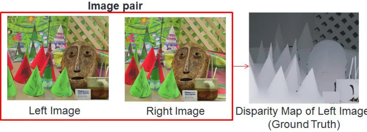
By experiments, we find the proper values for all the adjustable parameters in each system block. In the first system block, as mentioned previously, we pay attention to the results achieved by cost aggregation in order to keep the details. Hence, the adaptive window size N is set to 7. The scalar β for the smoothness term is set to 0.01. The iteration times T is 1. In the second system block, we pay attention to refining textureless pixels. Hence, the adaptive window size N is set to 7. The scalar β for smoothness term is set to 0.5 for computing left image disparity map and 0.4 for computing the right image disparity map. In order to refine the results of textureless pixels properly, the iteration times T is set to 2. In the third system block, we pay attention to solving the occlusion problem. Hence, the PID is used here. The adaptive window size N is set to 1. The scalar β for smoothness term is set to 3. The iteration times T is 1.

There are four commonly used test patterns from the Middlebury website [1], as shown in Figure 4-1. Their ground truths are shown in Figure 4-2. We will show the results of each system block and discuss the final results pattern by pattern. Finally, we will show the evaluation results on Middlebury [1] and also discuss them.

(40)

(41)

Figure 4-2 Ground truths: (a) Tsukuba ground truth, (b) Venus ground truth, (c) Teddy ground truth, (d) Cones ground truth.

First, we discuss the image pair of Tsukuba. Tsukuba has a rough background but continuous values of disparity. Some parts of the table lamp, such as its brace, are so narrow and may get merged into nearby regions. To prevent merging these narrow parts into nearby regions, the result obtained by cost aggregation is important; that is, the result of the first system block is important. Figure 4-3 shows the output of the first system block. The output shows that the disparity values of those narrow parts can be kept instead of being merged into nearby regions, but the disparity values of the background are not smooth. This problem will be solved in the second or third

(42)

system block. Figure 4-3(c) and (d) show the confidence maps for the next system block.

Figure 4-3 Outputs of the first system block: (a) initial disparity map of left image, (b) initial disparity map of right image, (c) confidence map of left image, (d) confidence map of right image.

In the second system block, we focus on refining the disparity values based on the results of the first system block. Here, we try to make most of the disparity map smooth and try to deal with the textureless regions. There are two iterations in this block in order to solve the textureless problem properly. The output results are shown as Figure 4-4. Most parts of the disparity map are getting smooth and those narrow parts, such as the braces of the table lamp, remain. However, some regions still have incorrect disparity values, like the wire between the lamp and its brace. The wire cannot be seen clearly in the output disparity map and cannot be refined anymore. Moreover, there are still some parts with strange disparity values, such as

(43)

those parts at the left side of some objects in Figure 4-4(a). These parts are so-called occlusion pixels and will be handled in the third system block. Figure 4-4 (c) and (d) show the confidence maps. Figure 4-4 (e) and (f) show those pixels with inconsistent disparity values.

Figure 4-4 Outputs of second system block: (a) disparity map of left image, (b) disparity map of right map, (c) confidence map of left image, (d) confidence map of right map, (e) PID map of left image, (f)

PID map of right map.

In the third system block, we focus on refining those pixels with wrong disparity values. Most of these pixels are the occluded pixels. The final results are shown in Figure 4-5. As expected, the pixels at the left side of objects that have strange disparity values can be refined properly. In Figure 4-6, we compare our result with

(44)

the ground truth. The black regions in the ground truth are the pixels with unknown disparity values. In addition to the missing wire between the lamp and its brace, there are still some obvious pixels with wrong disparity values, such as the square block at the right side of the table and some pixels between the braces of the table lamp. We have submitted the estimated disparity maps of the four test patterns to Middlebury for quantitative comparison. The result of Tsukuba pair performs better than the other three. The detail will be discussed later.

Figure 4-5 Outputs of the third system block: (a) disparity map of left image, (b) disparity map of right image.

(45)

The second test pattern is called Venus, which has lots of textureless regions and much smoother disparity values. The disparity map of Venus can be categorized into four blocks. For the textureless regions, traditional local algorithms often estimate wrong disparity values for these pixels above the newspaper in the image. This problem will be solved by global algorithms. Figure 4-7 shows the outputs of the first system block. As mentioned before, many pixels above the newspaper have no confident disparity values as shown in Figure 4-7 (c) and (d). These regions will be solved in the second or third system block.

The results of the second block are shown in Figure 4-8. As shown in Figure 4-8 (c) and (d), the textureless pixels problem mentioned above can be solved in this system block. The occlusion problem is left to be solved in the third block.

(46)

The output results of the third system are shown in Figure 4-9. Most of the aforementioned problems have been solved. However, while comparing with the ground truth as shown in Figure 4-10, we can find that there are still some pixels which don’t have smooth disparity values. This happens at the regions which get inconsistent disparity in the last system block. For example, this happens at the edge of the newspaper. This region can be refined properly by increasing the value of the

(47)

scalar parameter β of the smoothness term in the third system block. However, although a higher value of the scalar parameter can solve this problem, it may cause the narrow regions in the other test patterns to be merged into nearby regions, such as the braces of the lamp in the Tsukuba pair. Therefore, we still choose the previously proposed parameter set to test all four test pairs.

(48)

The third test pattern is called Teddy. The challenging areas of this test pattern are the sealed region below the chimney and the region at the right side of the teddy bear. These regions contain lots of pixels with no specific textures. The region at the right side of teddy bear can be refined properly in the proposed second or third system block. The most difficult problem to solve is the region below the chimney. Most pixels of this region are occluded by the foreground objects, while the remaining unoccluded pixels have little texture. To solve this problem, we use mainly the cost aggregation term and set the adaptive window size N to 7 to obtain more information in the first system block. The result of the first system block is shown in Figure 4-11. After that, we try to refine this region by these pixels with correct disparity value. Here, we assign a value around 0.5 to β. However, the final determination of β in this system block is decided when we consider the fourth pattern. Furthermore, to refine the disparity map properly, we set the iteration number T to 2 in the second system block. The output results of the second system block are shown in Figure 4-12. The third system block solves the occlusion problem and its output results are shown in Figure 4-13, where the problems mentioned previously can be handled properly.

(49)

(50)

While comparing the results with the ground truth as shown in Figure 4-14, we still find some problems in our results. Although the disparity values of the region below the chimney are not assigned to the disparity value of the chimney anymore, this region still has wrong disparity values. Another region with apparent wrong disparity values is at the left side of the left image. Since this region cannot be seen in the right image, this region has wrong disparity values and is not properly refined in the third system block.

(51)

The fourth test pattern is called Cones. The challenging areas of this pattern are the region with multiple cones and the region of the chopsticks. The region with multiple cones has lots of occluded pixels while the region of the chopsticks is narrow. The methods for solving these challenges are the same as the methods used to solve the challenges of the last three patterns. All we have to do is to find the proper parameters for the four patterns. The exact scalar parameter β in the second system block is decided here in order to refine the disparity map of the chopsticks region. The output results of the first system block are shown in Figure 4-15. Figure 4-16 shows the output results of the second system block and Figure 4-17 shows the output results of the third system block.

(52)

(53)

Then, we compare the final result with the ground truth as shown in Figure 4-18 and identify some problems of our results. Although the region of the chopsticks is refined properly, the region near the chopsticks has wrong values of disparity. Another obvious region with wrong disparity values is at the left side of the left image. The reason for this problem is the same as that when comparing the results of the third pattern with the ground truth.

Figure 4-18 Cones: (a) disparity map of our method, (b) ground truth.

Finally, we submit our results to Middlebury to compare our results with the results obtained by other methods. The results submitted to Middlebury are listed in Table 4-1, 4-2, 4-3 and 4-4. The case that achieves the best rank in our proposed method is Tsukuba. When the error threshold, which means the allowable difference of disparity values between our results and the ground truth, is set to 0.5, the rank for our method for Tsukuba is 22. From the results submitted to Middlebury, we can find that when the threshold error is set to a lower value, which means the allowable

(54)

difference is low, we can achieve higher ranks. When the threshold error is set to a higher value, we achieve a lower rank. A possible reason for this result may be that some of the other methods set the disparity values to be a real value, while our method only allows integer values.

Table 4-1 Results of Tsukuba on Middlebury

Error Threshold

Tsukuba

(without occluded pixels)

Tsukuba (all) Percentage of Bad Pixels Rank Percentage of Bad Pixels Rank 0.5 9.97 22 11.7 24 0.75 9.97 35 11.7 38 1 3.05 97 4.08 91 2 1.88 88 2.41 77

Table 4-2 Results of Venus on Middlebury

Error Threshold

Venus

Venus (all) Percentage of Bad Pixels Rank Percentage of Bad Pixels Rank 0.5 7.58 72 8.70 80 0.75 2.17 94 3.18 95 1 1.48 101 2.26 97 2 0.47 87 0.89 86

(55)

Table 4-3 Results of Teddy on Middlebury

Error Threshold

Teddy

Teddy (all) Percentage of Bad Pixels Rank Percentage of Bad Pixels Rank 0.5 13.9 51 21.0 59 0.75 9.28 65 16.2 73 1 7.80 71 14.2 82 2 5.09 72 9.48 87

Table 4-4 Results of Cones on Middlebury

Error Threshold

Cones

Cones (all) Percentage of Bad Pixels Rank Percentage of Bad Pixels Rank 0.5 9.87 61 17.0 61 0.75 5.91 75 12.9 78 1 4.89 85 11.4 81 2 2.99 71 8.11 70

(56)

Chapter 5 Conclusion

In this thesis, we propose a system to solve the challenges of stereo matching with a proposed matting affinity based stereo matching algorithm. First, we redefine the global cost function for our proposed global algorithm and develop the proposed method to solve this global optimization problem. Second, we construct a system with three system blocks. Each block has its own role to solve the stereo matching problems. The first system block pays attention to the result of cost aggregation. The second system block pays attention to refining the estimated disparity map in the first system block and to solving the textureless problem. The third system block pays attention to solving the occlusion problem. For each block, we have properly adjusted the four kinds of parameter: adaptive window size N, scalar β for smoothness term, iteration numer T, and the PID. The experimental results have demonstrated that our proposed system can successfully solve most of the textureless problem and the occlusion problem.

(57)

Reference

[1] Daniel Scharstein and Richard Szeliski, “The Middlebury Computer Vision Pages,” http://vision.middlebury.edu/stereo/, August 15, 2009.

[2] R. Szeliski, Computer Vision: Algorithms and Applications (Texts in Computer Science). Springer-Verlag London Limited, 2011.

[3] D. Scharstein and R. Szeliski. A taxonomy and evaluation of dense two-frame stereo correspondence algorithms. International Journal of Computer Vision, 47(1/2/3):7-42, April-June 2002

[4] X. Mei, X. Sun, M. Zhou, S. Jiao, H. Wang, and X. Zhang, “On building an accurate stereo matching system on graphics hardware,” International Conference on Computer Vision 2011.

[5] K. Zhang, J. Lu, and G. Lafruit, “Cross-based local stereo matching using orthogonal integral images,” IEEE Transactions on Circuits and Systems for Video Technology, 19(7):1073–1079, 2009.

[6] M. Bleyer, C. Rhemann, and C. Rother, “PatchMatch stereo - stereo matching with slanted support windows,” British Machine Vision Conference 2011

[7] A. Levin, D. Lischinski, Y. Weiss, “A Closed Form Solution to Natural Image Matting,” IEEE T. PAMI, vol. 30, no. 2, pp. 228-242, Feb. 2008.

[8] Chen-Yu Tseng, Sheng-Jyh Wang, “A cell-based matting Laplacian for contrast enhancement,” in IEEE International Conference on Image Processing (ICIP), 2012.

[9] Z. Wang and Z. Zheng, “A region based stereo matching algorithm using cooperative optimization,” IEEE Conference on Computer Vision and Pattern Recognition 2008.

[10] M. Bleyer, C. Rother, and P. Kohli, “Surface stereo with soft segmentation,” IEEE Conference on Computer Vision and Pattern Recognition 2010.

[11] W. Chen, M. Zhang, and Z. Xiong, “Segmentation-based stereo matching with occlusion handling via region border constrains,” Computer Vision and Image Understanding 2009

[12] Olga Veksler and Andrew Delong, software for energy minimization with graph cuts Version 3.0, 2010

(58)

[13] Yuri Boykov and Olga Veksler , http://vision.csd.uwo.ca/code/

[14] F. Besse, C. Rother, A. Fitzgibbon, and J. Kautz, “PMBP: PatchMatch belief propagation for correspondence field estimation,” British Machine Vision Conference 2012

[15] R. Kimmel, R. Klette, and A. Sugimoto, “Efficient Large-Scale Stereo Matching,” Asian Conference on Computer Vision 2010, Part I, LNCS 6492, pp. 25–38, 2011.

[16] D. Scharstein and R. Szeliski. High-accuracy stereo depth maps using structured light. In IEEE Computer Society Conference on Computer Vision and Pattern Recognition (CVPR 2003), volume 1, pages 195-202, Madison, WI, June 2003. [17] D. Scharstein and C. Pal. Learning conditional random fields for stereo. In IEEE

Computer Society Conference on Computer Vision and Pattern Recognition (CVPR 2007), Minneapolis, MN, June 2007.

[18] H. Hirschmüller and D. Scharstein. Evaluation of cost functions for stereo matching. In IEEE Computer Society Conference on Computer Vision and Pattern Recognition (CVPR 2007), Minneapolis, MN, June 2007.

[19] Y. Boykov, O. Veksler, R.Zabih, “Efficient Approximate Energy Minimization via Graph Cuts,” IEEE Transactions on Pattern Analysis and Machine Intelligence , 20(12):1222-1239, Nov 2001.

[20] V. Kolmogorov, R.Zabih, “What Energy Functions can be Minimized via Graph Cuts?” IEEE Transactions on Pattern Analysis and Machine Intelligence, 26(2):147-159, Feb 2004.

[21] Y. Boykov, V. Kolmogorov, “An Experimental Comparison of Min-Cut /Max-Flow Algorithms for Energy Minimization in Vision,” IEEE Transactions on Pattern Analysis and Machine Intelligence, 26(9):1124-1137, Sep 2004.

以去背相連性為基礎之立體匹配研究

國 立 交 通 大 學

電子工程學系 電子研究所碩士班

碩

士

論

文