Space-decomposition minimization method for large-scale minimization problems

(1)

computers &

mathematics

vmh smk.dkme P E R G A M O N Computers and Mathematics with Applications 37 (1999) 73--88

Space-Decomposition Minimization

M e t h o d for Large-Scale Minimization Problems

C H I N - S U N G LIU

Research Assistant of Applied O p t i m u m Design Laboratory D e p a r t m e n t of Mechanical Engineering, National Chiao T u n g University

Hsinchu 30050, Taiwan, R.O.C. C H I N G - H U N G T S E N G

Professor of Applied O p t i m u m Design Laboratory

D e p a r t m e n t of Mechanical Engineering, National Chiao T u n g University Hsinchu 30050, Taiwan, R.O.C.

(Received August 1997; accepted September 1998)

A b s t r a c t - - T h i s paper introduces a set of new algorithms, called the Space-Decomposition Min- imization ( S D M ) algorithms, that decomposes the minimization problem into subproblems. If the decomposed-space subproblems are not coupled to each other, they can be solved independently with any convergent algorithm; otherwise, iterative algorithms presented in this paper can be used. Fur- thermore, if the design space is further decomposed into one-dimensional decomposed spaces, the solution can be found directly using one-dimensional search methods. A hybrid algorithm that yields the benefits of the S D M algorithm and the conjugate gradient method is also given.

A n example that demonstrates application of S D M algorithm to the learning of a single-layer perceptron neural network is presented, and five large-scale numerical problems are used to test the S D M algorithms. The results obtained are compared with results from the conjugate gradient method. (~) 1999 Elsevier Science Ltd. All rights reserved.

K e y w o r d s - - U n c o n e t r a l n e d minimization, Decomposition method, Direct-search method, Large- scale problem.

1. I N T R O D U C T I O N

This paper introduces a set of space-decomposition minimization (SDM) algorithms for solving the unconstrained minimization problem

min f(x), (1)

z E R ~

where f : ~n ~ ~ is a lower bounded and continuously dilferentiable function.

The space-decomposition minimization (SDM) algorithms are based on decomposing the design space S 6 ~'* into individual subspaces. The minimization problem can then be decomposed into q subproblems and the final minimization solution is the combination of the q decomposed- space minimization solutions.

The research reported in this paper was supported under a project sponsored by the National Science Council Grant, 'Palwan, R.O.C., N S C 85-2732-F_,-009 -010.

(2)

74 C.-S. LIu AND C.-H. TSZNG

The space-decomposition minimization (SDM) algorithms can be considered as extensions of the Parallel Variable Distribution (PVD) algorithm and associated decomposition methods. The P V D algorithm, proposed by Ferris and Mangasarian [1], and extended by Solodov [2], is a method that decomposes the design variable x into q blocks xl,..., xq and distributes them

among q processors, where xt E ~ nt with ~"~=I nt = n. Mangasarian [3] also introduced a

method that assigns a portion of the gradient Vf(x) to q processors. Similarly, the n-dimension real-space Nn is also decomposed into q hi-dimension subspaces.

Decomposition methods for decomposing the minimization problem into subproblems have been proposed by several researchers. Kibardin [4] decomposed minimization problem (1) into f(x) = ~~=i fi(x), where x E Nn and fi(x) is a convex function. Mouallif, Nguyen and Strodiot [5] also

decomposed minimization problem (1) into, where f(x) -- fo(X) + ~-~=1 fi(x), where x E Nn,

f0 is a differentiable, strongly convex function, and fi(x) is a convex function. In these studies,

the computing efficiency was shown to increase when the original minimization problem could be decomposed into subproblems.

In this paper, the P V D algorithm and the decomposition methods are combined into the space-decomposition minimization (SDM) algorithms. It is shown that any convergent algorithm that satisfies the descent condition can be applied to solve the decomposed-space subproblems. In addition, if the design space is further decomposed into one-dimensional decomposed spaces, one-dimensional search methods can be used directly to solve the subproblems. That is, the S D M algorithm can be considered a direct search method.

Direct-search methods search for m i n i m u m solutions directly without requiring analytic gradient information. The multiple mutually conjugate search directions are commonly used in the direct search methods [6-8]. Line search along these multiple search directions can be evaluated simultaneously on different computers using only evaluation of minimization function. In this paper, the special pseudo-conjugate directions [9] that parallel the coordinate axes are used for the direct-search S D M algorithm, and one-dimensional search methods, including exact and nonexact methods, can be used directly to solve the one-dimensional subproblems.

This paper is organized as follows. The space-decomposition minimization (SDM) algorithm is presented in Section 2. The direct-search space-decomposition minimization (direct-search S D M ) algorithm is presented in Section 3. In Section 4, a hybrid S D M algorithm that combines the algorithms presented in Sections 2 and 3 is introduced. A n example of application to the neural networks is given in Section 5, and numerical experiment results are given in Section 6. The conclusions along with further research directions are given in Section 7, and all test problems are listed in the Appendix.

The notation and terminology used in this paper are described below [3].

S E Nn denotes n-dimensional Euclidean design space, with ordinary inner product and associated two-norm [[ • [[. Italic characters denoting variables and vectors. For simplicity of notation, all vectors are column vectors and changes in the ordering of design variables are allowed through- out this paper. Thus, the design variable vector x E S can be decomposed into subvectors. That

is, x = [ x s l , . . . , xs~] T, where xs~ are subvector or subcomponent of x.

2. S P A C E - D E C O M P O S I T I O N

M I N I M I Z A T I O N ( S D M ) A L G O R I T H M

The space-decomposition minimization algorithm is based on the nonoverlapping decomposed- space set and the decomposed-space minimization function defined below.

DEFINITION 2.1. NONOVERLAPPING DECOMPOSED-SPACE SET. For the design space S spanned by {x [ x E ~"}, if the design variable x is decomposed into x = [xsl,... ,xs,] T, then the decomposed space Si spanned by {xsi [ xs~ 6 ~ " ' , where ~"~=lq n~ = n} forms a nonoverlapping

(3)

Space-Decomposition Minimization Method 75

decomposed-space set {$1, .... Sq}. That is, q

U S , = S

and

S~nSj=O,

ifi~j.

Moreover, the complement space of S~ is defined as

Si

spanned by

{x&

] where

_- x).

(2)

That is, Si U Si = S and :~i n S~ = 0, V i e (1, q).

According to definitions of the nonoverlapping decomposed-space set, the minimization function (1) can be decomposed as

f(x) = f$, (xS,,x~,) -t-f~, (x~,). (3)

where fs,(xs,, x&) is the decomposed-space minimization function and fg, (xg,) is the complement decomposed-space minimization function.

COROLLARY 2.2. According to (3), the complement decomposed-space minimization function f&(xg, ) is only a function of x&. That is, f i x & /s a constant vector, f&(x&) can be treated as a constant value that can be removed during the process of minimizing decomposed-space subproblems.

The following example uses the Powell test function listed in the Appendix to describe Defini- tion 2.1 and Corollary 2.2.

EXAMPLE 2.3. The Powell minimization problem with four design variables is [9-11]. min f(x) = (Xl -{- 10x2) 2 -[- 5(x3 - x4) 2 -{- (x2 - 2x3) 4 -{- 10(Xl - x 4 ) 4.

zER 4

Definition 2.1 and Corollary 2.2 suggest the nonoverlapping decomposed spaces Si, i = 1 , . . . , 4, are spanned by {Xl), {x2}, {x3), {x4}, and the complementary spaces •, i = 1 , . . . , 4 , are spanned by {x:,xa,x4), {xl,xa,x4}, (xl,x2,x4}, {xl,x2,x3), respectively. Thus, the decomposed-space minimization function f& can be expressed by eliminating the component of f(x) defined only in S~. That is,

IS1 (XSI,X~I) -~ (Xl -}- 10X2) 2 "{- 10(xl - x4) 4,

= + 2 + -

4,

f s s (XSa, X~s) ---- 5(X3 -- X4) 2 -4- (X 2 -- 2X3) 4,

IS4 (Xs,, X,~4) ---~ 5(X3 -- X4) 2 + 10(Xl -- X4) 4.

These subproblems can then be solved using the methods presented in this paper. | The definition of the nonoverlapping decomposed-space set leads to the following theorem. T H E O R E M 2.4. U N C O U P L E D S P A C E - D E C O M P O S I T I O N T H E O R E M . //'minimization

problem (1)

can be decomposed

into

q

f(x) = ~ f& (XS,), (4)

iffil

where {81,..., Sq } is the nonoverlapping decomposed-space set, then the minimization prob- lem (1) can be decomposed into q uncoupled subproblems that can be solved independently

using any convergent a/gorithm. That is,

(4)

76 C.-S. LIu A N D C.-H. TS~.NG

and the final minimization or stationary solution can be obtained from

x" [ * . . x * ] T

= = s , , . , s ,

(6)

PROOF. From (4), it gets

0 / ( = ) = Ofs,(=s,) v x j E s~.

(7)

Oxj Oxj '

Thus, from Definition 2.1 and (7), it can be concluded that

Of(x) 0Is, (xs,)

0=-"-7 = o=~ ' v=~ e s.

(8)

Since x~, is the minimization solution for decomposed space Si, it follows that x*

0fs, ( s , ) = 0, Vxj 6 S,. (9)

Oxj

Thus, from (8) and (9), it can be concluded that

Of (x*)

Ox----7- " = O, V xj E S.

That is, [[Vf(x*)][ = 0, and this is the minimization or stationary condition for minimization

problem (1). |

Theorem 2.4 is efficient for some simple problems, and can save lots of processor time and memory resources. However, most minimization problems cannot be decomposed into uncoupled decomposed-space subproblems, so iterative algorithms must be used.

Before stating and proving the iterative space-decomposition minimization algorithm, the definition of forcing function [1,3] is required and is defined below.

DEFINITION 2.5. FORCING FUNCTION. A continuous function a from the nonnegative real line

into itself is said to be a forcing function on the nonnegative real-number sequence {~} if a ( 0 ) = 0 , w i t h { a ( ~ ) } > 0 f o r ~ > 0 . (10)

In addition, a ( ~ ) --* 0 implies {~i} --* 0.

The forcing function definition leads to the following space-decomposition theorem and proof. THEOREM 2.6. SPACE-DECOMPOSITION THEOREM. If the design space S 6 @%" of n~nirnization

problem (1) is decomposed into a nonoverlapping decomposed-space set { S , , . . . , Sq}, then mini-

mization problem (1) can be solved iteratively in the q decomposed spaces using any convergent algorithm that satisfies the descent condition [3]:

k T ~

([W/s,

( 1 1 )

- V f s , (Xs,,XS,) ds, >_ a] and

(X k+l ( - - V f$, (xk,,x,~,) T d k ) > 0, (12)

f$, (x~,,x~,) - f$,l, S, ,x~,) _> 0"2

where d k & is the search direction in decomposed-space S~, (71 is a forcing function on the se- quence { II V / s ,

(=~,, =;, )11 },

~2 is a forcing function on the sequence { - V / s ,

(=~,, =~, )rd~, },

and

X k+l X _s,_, _&]IT _{= i s , ,}rXk = _&]~T _{+ a k d ~ , in space S~.}

The final minimization or stationary solution can be obtained by directly combining the solu- tions of the q subproblems. That is, x* = [Xsl, , ... ,Xsq ] . m.

(5)

S p a c e - D e c o m p o s i t i o n M i n i m i z a t i o n M e t h o d 77

PROOF. Using (12) and the forcing function definition yields

(Xs, ,xg,) -< Ss, (x~,,xg,).

(13)

fs~ k+l

Expanding (13) using the Taylor series about point x ~ yields

.fs, (x~,,x~,) +ak (c~, .d~,) _< .fs, (x~,,x~,),

(14)

where c~, is the gradient of fs, (x~,, xg,) in space S,. Thus, the descent condition for S, can be obtained as [12]

_< o (15)

Since ak > 0, it can be rewritten as

_< o. (16)

That is, (13) and (16) are equivalent. From (7) and (8), it gets

Since

d k

= [ s l , " " ,d~q] T, from (16) and (17) it gets that

d k

q

ck" dk = Z

(c~,. d~,) <

0.

(18)

'/,----1

That is, the descent condition is also satisfied in design space S and it can be concluded that

f

(x k+l) <

f

(xk). (19)

Therefore, {f(xk)}, is a nonincreasing sequence. Since

f ( x k)

is a lower bounded function, it gets from (19) that 0 = lim

[$

(x k) -

.f (xk+')]

k---*oo q {xk+l~] = k-.oolim ~ [f (xk,) -- f ~, s, ]J (20) i----1 q

> lim

~'a~(--Cks,.dks, )

> 0 , (by(12)). - - k--*oo ~

i = 1

Thus, from (20) and the forcing function definition, it gets

lim ( - c k, .dk,) = 0 , Vi E (1,q). (21) k - * o o

Using (11) and (21), it gets

0 = lira (-~s, "dk,) > lira al

(11411)

> 0.

(22)

k - . o o - - k--,oo - -

Therefore, forcing function definition yield [l~&[[ = 0. From (17), it can be concluded that I[ckl[ = 0. That is,

[[Vf(xk)[I

= 0, and the minimization or stationary solution can be obtained a s

l i r a [ I x k ' b l - x k [ [ ---- O. m k--.oo

In general, finding the exact zero point of [[Vf(xk)[[ is either impossible or impractical for numerical methods. Thus, the following convergence criteria can be applied to solve all the decomposed-apace subproblems [13]:

I. Max {[[V fs,(x~,,xg,)[[,i = 1,... ,q} < e,

II. [[Vf(xk)[[ <_ e, where xk ---- [xk81 ' " " ' ' xk8, J1T'

k+l - (x~,)j[ _< e([(x~+l)j[ + 1), where (.)j denotes the jth component of

xs,.

(6)

78 C.-S. Lxv AND C.-H. TSENO

It has been shown that T h e o r e m 2.6 can be applied to minimization problem (1) even though the decomposed-space minimization functions are coupled to each other. T h e o r e m 2.6 can be summarized as the following algorithm.

A L G O R I T H M 2.7. S P A C E - D E C O M P O S I T I O N MINIMIZATION ( S D M ) A L G O R I T H M .

Step 1. D e c o m p o s e the design space into a nonoverlapping decomposed-space set

{$I,...,

Sq}.

Step 2. Derive the decomposed-space minimization functions

f& (xs~,

xg~),

for { = 1,..., q. Step 3. Choose the starting point x I, where x I = [ S l " ' ' ' X 1 xlsq] T and set k -- 1.

t t x k ' i X x

Step 4. For i = 1 to q, solve one or more steps of the minimization subproblems Js~t s~, ~,) using any convergent algorithm, such as the conjugate gradient method, t h a t satisfies descent conditions i l l ) and (12). Then, update Xs,k'i, which is the subvector of xk; that is,

X k [ x k , 1 _ k , q l T -~ t Si ' ' " " X S q l "

Step 5. Apply convergence criterion to all decomposed-spaces Si. If the convergence criterion is satisfied for all decomposed spaces, then the minimization solution has been found as x* = [X's1, "'" , X*sqj]T', otherwise, set k = k + 1 and go to Step 4.

3. DIRECT-SEARCH

S P A C E - D E C O M P O S I T I O N

MINIMIZATION (SDM) ALGORITHM

Since direct-search methods with no analytic gradient information are of interest to a number of researchers, a direct-search SDM algorithm is also introduced in this paper.

It has been shown that, if the design space S is further decomposed into a one-dimension decomposed-space set { $ 1 , . . . , S , } , V S~ E !!~ 1, one-dimensional search methods can be directly applied to Step 4 of Algorithm 2.7, and search direction updating can be eliminated. T h a t is, the minimization function gradient is not required. T h e direct search algorithm is illustrated as the direct-search SDM algorithm below.

ALGORITHM 3.1. DIRECT-SEARCH S D M ALGORITHM.

Step 1 to 3 are the same as those in Algorithm 2.7 except for setting q = n.

Step 4. For i -- 1 to n, solve the minimization solutions x kJ & using any one-dimensional search m e t h o d t h a t satisfies

[ k,~

Ss, ~,Xs, ,x~,) <

Ss, (xks,,x~,) •

(23)

Then, u p d a t e x k'i which is the subcomponent of _{S i} xk; t h a t is, x k ₌ Ix k'z _t _{$ 1} _{' " " " ' " ~ S t t J}"k'nlT _" Step 5. Check the convergence criteria

max ISs,

(x~,,x~,) - Ss,

(x~, + ~,x~,)l < ~ ,

(24)

iE(1,n)

o r

- + 2 <

i----1

where 6 and ~ are small positive values. If the convergence criterion has been satisfied,

• X* | T .

t h e n the minimization solution has been found as x* = [ x s ~ , . . . , s.J , otherwise set k = k + 1 and go to Step 4.

In the direct-search SDM algorithm, x ~ is used as the line search parameter, and any exact or inexact line search method satisfied (23) can be used. This is a special case of Algorithm 2.7. T h e advantages are t h a t the search direction is either +1 or - 1 , depending only on the sign of fs, (xk~, x~,) -- f S , ( x ~ + 6, x ~ ) , where if is a small positive real number. Only one-dimensional search methods are used in every decomposed-space Si, and the convergence of Algorithm 3.1 can

(7)

be proof by Theorem 2.6 with all the dimensions of decomposed space are set to one. In addition, if the gradient of any decomposed-space minimization function ~ = 0 can be explicitly expressed

d x s i

as x & = g ( x & ) , then x s , can be calculated directly without using any one-dimensional search method.

4. H Y B R I D S P A C E - D E C O M P O S I T I O N

M I N I M I Z A T I O N A L G O R I T H M

As shown in Figures 1 and 2, the direct-search SDM algorithm initially decreases the minimization functionis value far faster t h a n the conjugate gradient method does. However, the direct-search SDM algorithm converges more slowly t h a n the conjugate gradient method around

100 : ...

• ... Conjugme Gradient Method

IO

,,

• .

~

Non-gradient SDM AIgorflhm

u 1

~

.

"...%

.

"'~-" Stage II of Hybrid S D M Algori@an

o.1

.~

o.o,

0.001 '~

0.00001

i

':

o.ooooo

i

0 . 0 0 0 0 0 0 1 ' '": ' ' ' 0 0.1 0.2 0.3 0 . 4 0.5 0 . 6 0.7

Sec.

Figure 1. Minimization function value versus time for problem (6) when n = 20.

1oooo

1

--. .... . ~ N o n - ~ m SDMAls~ridan ~

I

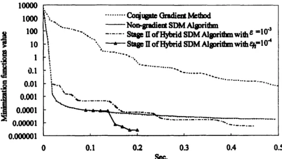
I00 ~ " ""-,. - ... Stalle IIofHybridSDMAlgorithmwilh ~ =I0" I I0 !L " " " - StagelI°fHybridSDMAIsm'iltanwitheh=104 I

0.I

0.01 .

~

...

0.001

'"",...

...

.

0.0001

"~

0.00001 . 4 . . . .

...

0.000001 ' ' ' 0 0.1 0.2 0.3 0.4 0.5

See.

Figure 2. Minimization function value versus time for time for text problem (I) when n = 100.

(8)

80 C.-S. LIU A N D C.-H. T S E N G

the minimization point. Thus, a hybrid algorithm that combines the benefits of both algorithms is presented below.

ALGORITHM 4.1. HYBRID SPACE-DECOMPOSITION MINIMIZATION (HSDM) ALGORITHM. S t a g e I

STEP 1 to 4 are the same as the direct-search Algorithm 3.1.

Step 5. If f& (x~, x$~) > 0, V k, check the approximate convergence criterion Ss, (x~,, x~,) ~h Ss, (x~,,x~,)

[xk+ 1 < , (26)

otherwise, check the approximate convergence criterion

max IS~, (x~,,x~,) - Ss, (x~, + 6,x~,)l < ~ h , (27)

iE(1,n)

to all decomposed-spaces, where ~ and eh are small positive values. If the approximate convergence criterion has been satisfied for all decomposed spaces, then go to Step 6; otherwise go to Step 4.

S t a g e II

Step 6. Using the approximate minimization solution in Stage I as the starting point, and then applying other convergent algorithms, such as the conjugate gradient method or the Al- gorithm 2.7, to find the final minimization solution.

Hybrid Algorithm 4.1 includes two stages. In the first stage, direct-search Algorithm 3.1 is used to solve for the approximate minimization solution. Then, another algorithm that converges more rapidly around the minimization point can be applied to solve for the final minimization solution in the second stage.

5. A P P L I C A T I O N E X A M P L E

The SDM algorithms were applied to the learning of the single-layer perceptron neural network to demonstrate their effectiveness.

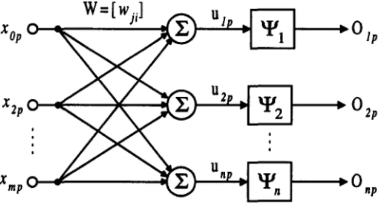
EXAMPLE 5.1. SINGLE-LAYER PERCEPTRON NEURAL NETWORK. The single-layer perceptron neural network with m input nodes and n output nodes shown in Figure 3 can be used as a pattern-classification device. The pth input pattern {x0p,..., Xrap} is multiplied by {wji}, which is a set of adjustable synaptic weights connecting the ith input node to the jth output node.

. w = [ wJ ] u Xop o - 1 I ~- 0 lp u 2

xzpc

2 I

~ O2p

,.

U n X rap 0 : 0 ,p

(9)

Space-Decomposition Minimization Method 81 Then, the internal potential ujp generated at the

jth

output node for the

pth

input pattern, is evaluated using

m

= (wj,x,p), (2s)

,=0

and the output YJn E ( 1 , - 1 ) is generated either via hard limiter yjp = sign (u~p),

or sigmoid function

YJn = tanh(Tujp), 7 > 0. (30)

Then, the output YJn is compared with the desired signal, d ¢ n • (1,-1), and the quantized error

ejp = din - YJn (31)

is generated to adjust the weight.

The standard perceptron neural network learning algorithm minimizes the mean-squared error function. Such a mean-squared error function for the f h pattern can he formulated as

1 n

Ep = ~ ~ e2n, (32)

jffil

and the total error function for all ~ patterns is formulated as

E = )--~Ep= ~ E ejp. 2 (33)

p=l p=l j=l

In order to apply uncoupled space-decomposition T h e o r e m 2.4 to minimize the total error function, (33) can be rewritten as

E = ~ ~ ej 2 = ~ Ej, (34)

j=l p=l j = l

where Ej = ~-~n--1 ejp = y~p=l(dj p _ yjp)2 is the error function generated at the jth output node ~ 2 for all input patterns.

Since YJn is a function of {wj0,..., wjrn} only, it can be concluded on the basis of Theorem 2.4 that the original design space Sw spanned by {wji [ wji • ~(r~+l)×n, j = 1 , . . . , n, i = 0 , . . . , m} can be decomposed into n nonoverlapping decomposed-spaces Sw~ spanned by

{wj, I wj, E ~rn, i---- 0 , . . . , m , Vj • (1,n)}. (35) That is, LJ~'=l Sw~ = Sw and Sw~ N S ~ = q), if j # j. Then, the unconstrained minimization problem (34) can be decomposed into n uncoupled subproblems

Ej = v j • ( 1 , . ) . (36)

p=l

These n uncoupled subproblems can be solved independently either on a single processor or on parallel processors. In addition, any of the n uncoupled subneural networks can be trained using either the conventional steepest-descent gradient rule [14] or some other more efficient minimization algorithm, such as the conjugate gradient method [15,16].

(10)

82 C.-S. LIu A N D C.-H. T S Z N G

Furthermore, the direct-search Algorithm 3.1 or the hybrid Algorithm 4.1 can also be applied to these n uncoupled subproblems. To apply the direct-search Algorithm 3.1 or the first stage of Algorithm 4.1 to subproblems (36), the original design space Swj in (36) must be further decomposed into one-dimensional space S%~ that is spanned by the subset

I

v;

vj (1,m)}.

( 3 7 )

Then, the error function ejp in

(36)

can be further decomposed into e#p = d#p - y#p

= d i p - t a n h ( ' y u j p )

= d i p - t a n h 7 WjiXip

ie(1,m) and i@i / J

where ~-~ee(i,m)and i~i(~UJiXiP) is a constant value in the decomposed-space S%~ and can be evaluated only once during the minimization process in decomposed-space S%~.

6. N U M E R I C A L T E S T I N G

To demonstrate the S D M algorithms, five large-scale test problems [10,11,17,18] were solved using the direct-search Algorithm 3.1 and the hybrid Algorithm 4.1. The numerical test results are shown in Tables 1 and 2, along with the results from the conjugate gradient method for comparison.

The notation used in Table 1 is shown below: n -- number of variables, IT = number of iterations,

C P U -~ processor time measured in seconds. The speed-up factors used in Table 2 were calculated as follows:

Processor time for the conjugate gradient method

Speed-up factor 1 = Processor time for nongradient Algorithm 3.1 ' (38) Processor time for the conjugate gradient method

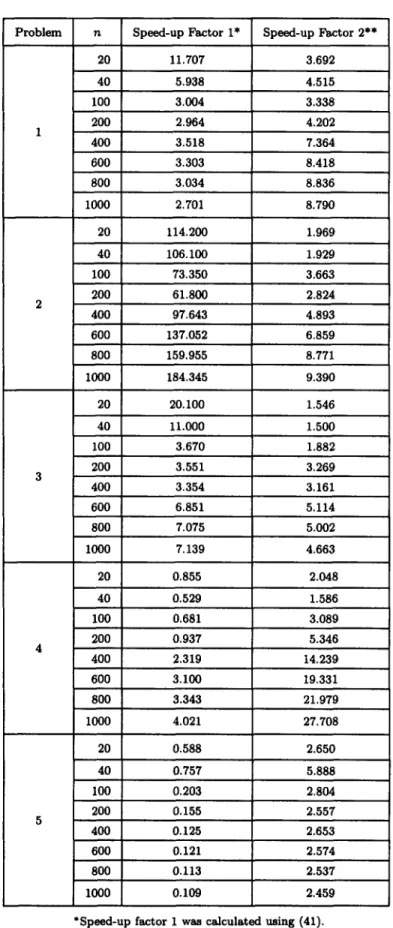
Speed-up factor 2 = Processor time for hybrid Algorithm 4.1 (39) As shown in Table 2, the speed-up factors varied from 0.109 to 184.345 for the direct-search S D M algorithm, and from 1.5 to 27.708 for the hybrid S D M algorithm. The numerical results were obtained on a Pentium 120 M h z machine with 48 M bytes of R A M memory, and the convergence criteria were set as e = 10 -3 and ~h -- 10 -3. The numerical test results show that the conjugate gradient method m a y be superior to direct-search S D M algorithm on some test problems. As shown in Figures 1 and 2, the direct-search S D M has a high convergence characteristic during the first few steps, but the convergence speed slows down significantly near the minimization point. However, as shown in Figures 1 and 2, the slow convergence problem of the direct-search S D M can be improved using the hybrid S D M algorithm. As Figure 2 shows, if the switch point between the two stages of hybrid S D M Algorithm 4.1 is properly chosen, the processor time can be significantly reduced.

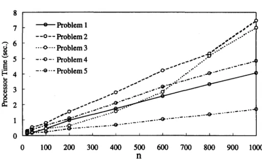
The processor times for the conjugate gradient method, the direct-search S D M algorithm and the hybrid S D M algorithm are shown in Figures 4-6, respectively. As Figure 1 shows, the

(11)

Space-Decomposition Minimization Method 83 Table i. C P U times and iteration numbers for the five test problems.

Direct-search S D M Conjugate Gradmnt

Hybrid S D M algorithm*

Problem n Algorithm Method*

IT C P U IT C P U I T 1 # I T 2 # # C P U 20 90 0.041 67 0.480 7 20 0.130 40 134 0.130 85 0.772 7 20 0.171 100 214 0.500 110 1.502 7 32 0.450 200 294 1.392 203 4.126 7 45 0.982 1 400 394 3.646 371 12.828 7 46 1.742 600 465 6.459 425 21.331 7 46 2.534 800 521 9.654 456 29.292 7 47 3.315 1000 569 1 3 . 1 9 9 459 35.651 7 47 4.056 20 13 0.005 66 0.571 3 31 0.290 40 13 0.010 108 1.061 3 49 0.550 100 14 0.040 210 2.934 3 51 0.801 200 15 0.070 212 4.326 3 63 1.532 2 400 15 0.140 416 13.670 3 68 2.794 600 15 0.210 616 28.781 3 69 4.196 800 16 0.291 814 46.547 3 69 5.307 1000 16 0.380 1008 70.051 3 80 7.460 20 27 0.010 26 0.201 14 16 0.130 40 32 0.030 42 0.330 14 26 0.220 I00 67 0.221 74 0.811 26 27 0.431 200 95 0.581 113 2.063 38 15 0.631 3 400 131 1.472 190 4.937 54 16 1.562 600 143 2.093 341 14.340 57 17 2.804 800 168 3.646 482 25.797 75 20 5.157 1000 187 4.566 495 32.597 77 19 6.991 20 593 0.551 63 0.471 20 30 0.230 40 615 1.172 73 0.620 20 42 0.391 100 643 3.045 147 2.073 20 42 0.671 200 664 6.229 246 5.838 20 44 1.092 4 400 685 12.849 760 29.803 20 49 2.093 600 697 19.608 1038 60.777 20 49 3.144 800 706 26.468 1161 88.487 20 49 4.026 1000 713 33.399 1447 134.303 20 48 4.847 20 959 0.631 53 0.371 6 19 0.140 40 998 1.322 129 1.001 6 19 0.170 100 1049 3.445 60 0.701 6 19 0.250 200 1087 7.090 61 1.102 6 19 0.431 5 400 1125 14.701 61 1.833 6 19 0.691 600 1148 22.532 61 2.734 6 19 1.062 800 1164 30.474 61 3.455 6 19 1.362 1000 1176 38.475 61 4.186 6 20 1.702

*Gradient information is assumed to be available for the conjugate gradient method and hybrid S D M algorithm.

# IT1 is the iteration number for Stage I of hybrid D S M Algorithm 4.1. # # IT2 is the iteration number for Stage II of hybrid D S M Algorithm 4.1.

(12)

84 C.-S. L]u AND C.-H. TSENO

Table 2. Speed-up factors for t h e five test problems.

Problem n Speed-up Factor 1" Speed-up Factor 2**

20 11.707 3.692 40 5.938 4.515 100 3.004 3.338 200 2.964 4.202 1 400 3.518 7.364 600 3.303 8.418 800 3.034 8.836 1000 2.701 8.790 20 114.200 1.969 40 106.100 1.929 100 73.350 3.663 200 61.800 2.824 2 400 97.643 4.893 600 137.052 6.859 800 159.955 8.771 1000 184.345 9.390 20 20.100 1.546 40 11.000 1.500 100 3.670 1.882 200 3.551 3.269 3 400 3.354 3.161 600 6.851 5.114 800 7.075 5.002 1000 7.139 4.663 20 0.855 2.048 40 0.529 1.586 100 0.681 3.089 200 0.937 5.346 4 400 2.319 14.239 600 3.100 19.331 800 3.343 21.979 1000 4.021 27.708 20 0.588 2.650 40 0.757 5.888 100 0.203 2.804 200 0.155 2.557 5 400 0.125 2.653 600 0.121 2.574 800 0.113 2.537 1000 0.109 2.459

*Speed-up factor 1 was calculated using (41). **Speed-up factor 2 was calculated using (42).

(13)

processor times for the conjugate gradient method are approximately exponential functions of the design variable numbers. By contrast, the processor times for the direct-search and hybrid SDM algorithms are approximately linear functions of the design variable numbers, as shown in Figures 5 and 6.

In order to compare the memory resources required by these methods, a Memory-Required Ratio (MRR) were calculated as follows:

Memory required for nongradient DSM Algorithm 3.1 (40) M R R = Memory required for the conjugate gradient method "

For minimization problem (1) with n design variables, it can be shown that the conjugate gradient method requires at least 3r~ units of memory to save the design variables, minimization function gradient and search-direction vector. Furthermore, additional temporary memory is required during the computation process for the conjugate gradient method. By contrast, the

140

, t

o Problem 1 _{B J}

120 - - o - - Problem 2 , / , "

100 ""<>"" Problem 3 ,-

"-" -..o-. Problem 4 .o"

.~ 80 -..o--- Problem 5 - " ' " • s S ( 60 ..o'"'" " 4° 20 0 200 400 600 800 1000 n

Figure 4. Processor times for the conjugate gradient method for different scales.

35 .,-"" o Problem 1 _{. . s °}.-" _{. ~ "},,~ 30 - - o - - Problem 2 . . a .-.'"" ,-v. ....o-.-- Problem 3 ..,-'" , ~ - ' " 25 ~o ,_,~ -. -o -- Problem 4 _{.°--" f . . . ' "}. , - ~ 20 -..o.-- Problem 5 . ° ~ ° °,~° . . - S - " ~ ..~ .*° 5 . . . 4 0 _ - " . . . ~ ' f ~ " . . . O " • . . . . ~ 0 " - - - ~ . . . . - " " . . . . " . . . . " ~ 0 100 200 300 400 500 600 700 800 900 1000 n

(14)

86 C.-S. LIU AND C.-H. TSENG 8 7 o Problem I ,**J~ ~ O .°° - -o - - Problem 2 ,,,,'..--" "-" 6 ...o--- Problem 3 -0"'"" ...

~

5 -.-o-- Problem 4 ,..-"'.'-" .- ~.,,, .°°° . . ~ ' ~ 4 - " o " " Problem5 ...o-- ..." . ..o. .. . . ~ 3

_{. - ' °}

-

_{...-'_...~...--~}

."" c r ' ~ 2 ~ , ' . " ~ " . . . -O" . . . 0 I I I [ 0 100 200 300 400 500 600 700 800 900 1000 n

Figure 6. Processor time for the hybrid DSM algorithm for different scales.

direct-search SDM algorithm requires only n units of storage memory to save the design variables and some more units of temporary storage for the one-dimensional search method.

Because temporary storage requirements are strongly dependent on programming techniques, the minimum amount of memory required was used to calculate the MRR. The MRR is less than 0.3333 as compared with conjugate gradient method. Therefore, the direct-search SDM algorithm is particular suitable for large-scale problems due to its low memory requirement.

7. C O N C L U S I O N S

Three fundamental convergent space-decomposition minimization (SDM) algorithms for large- scale unconstrained minimization problems have been presented in this paper. These algorithms allow minimization problems to be decomposed into q subproblems. If the decomposed-space minimization functions are uncoupled from each other, the q subproblems can be solved independently using any convergent algorithm. However, if they are coupled to each other, the iterative space-decomposition minimization (SDM) algorithm can be used and all subproblems can be solved iteratively with any convergent algorithm that satisfies space-decomposition Theorem 2.6. Furthermore, it has been shown that if the design space is further divided into one-dimensional decomposed spaces, general one-dimensional search methods can be applied directly to the one- dimensional subproblems, and the SDM algorithm can be considered a direct-search algorithm. Although the direct-search SDM algorithm converges slowly near the minimization point, the hybrid SDM algorithm can be used to eliminate the slow convergence problem.

Numerical tests have shown that the SDM algorithms save more processor time and memory resources than the conjugate gradient method. In addition, properly choosing the switch point between the two stages of the hybrid SDM algorithm allows the processor time to be significantly reduced, and further study of methods for finding the proper switch point for the hybrid SDM algorithm is warranted.

Although all of the test problems are solved on a serial computer, all of the algorithms presented in this paper are particularly suitable for parallel computers after further modification. Further study and testing on parallel computer of the SDM algorithms are warranted.

In the application example, the single-layer perceptron neural network was used as an example to demonstrate the effectiveness of SDM algorithms. However, the SDM algorithms can be extended to multilayer perceptron neural network by the multilevel decomposition methods [19,20] and further study and testing for multilayer pereeptron neural network are also warranted.

(15)

Space-Decomposition Minimization Method 87 A P P E N D I X

PROBLEM 1. EXTENDED POWELL TEST FUNCTION [9,10]. n/4

F = Z [(x4i-3 + 10x4i-2) 2 + 5(x4i-1 - x4i) 2 i=1

+ ( x 4 i - 2 - 2x4i-1) 4 + 10(x4/-3 - x4i)4] , x (1) = [ 3 , - 1 , 0 , 1 , . . . , 3 , - 1 , 0 , 1 , ] T .

PROBLEM 2. EXTENDED DIXON TEST FUNCTION [11].

= _ _ (1 - + (1 - + _ _ (x~. - X j + l ) 2 ,

F

/--1 j = 1 o i - 9

X (1) = [ - - 2 , - - 2 , . . . , - - 2 ] T .

PROBLEM 3. TRIDIA TEST FUNCTION [i0].

n

F =

Z[i(2x/-

x,_1)2],

i=2

X (1) = [3, - 1 , 0 , 1 , . . . , 3, - 1 , 0, 1] T.

PROBLEM 4. EXTENDED WOOD TEST FUNCTION [9,11]. n/4

F = Z { 1 0 0 ( x2/-3 - xa/-2) 2 + (xa/-3 - 1) 2 + 90 (x2/_1 - Xa,) 2 i=1

+ ( I - x4i_1) 2 -~- 10.1 [(x4i_ 2 - 1) 2 Jr ( x 4 / - 1) 2]

+ 19.8(x4/-2 - 1)(X4i -- I ) } ,

X ( I ) = [-3, - I , - 3 , - I , . . . , -3, - I , - 3 , -I] T.

PROBLEM 5. EXTENDED ROSENBROCK TEST FUNCTION [i0,II]. n/2

F ---- ~ - - L [100 (x2, -- X2i-1) -~- (1 2 2 _ X2i_I) 2]

/=1

X (I) = [--1.2, I, --1.2, i , . . - , --1.2, i] T. R E F E R E N C E S

1. M.C. Ferris and O.L. Mangasarian, Parallel variable distribution, SIAM J. Optim. 4 (4), 815-832, (1994). 2. M.V. Solodov, New inexact parallel variable distribution algorithms, Computational Optim. and Applications

7, 165-182, (1997).

3. O.L. Mangasarian, Parallel gradient distribution in unconstrained optimization, SIAM J. Contr. ~ Optim.

3 8 (6), 1916--1925, (1995).

4. V.M. Kibardin, Decomposition into functions in the minimization problem, Automation and Remote Control

40 (1), 1311-1323, (1980).

5. K. Mouallif, V.H. Nguyen and J.-J. Strodiot, A perturbed parallel decomposition method for a class of nonsmooth convex minimization problems, SIAM J. Contr. ~ Optim. 29 (4), 829-847, (1991).

6. D.G. Mcdowell, Generalized conjugate directions for unconstrained function minimization, J. Optim. Theory

and Applications 41 (4), 523-531, (1983).

7. Y.A. Shpalenskii, Iterative aggregation algorithm for unconstrained optimization problems, Automation and

Remote Control 42 (i), 76--82, (1981).

8. C. Sutti, Nongradient minimization methods for parallel processing computers, Parts 1 and 2, J. Optim.

(16)

88 C.-S. LIU AND C.-H. TSF.~G

9. E.C. Housos and O. Wing, Pseudo-conjugate directions for the solution of the nonlinear unconstrained opti- mization problem on a parallel computer, J. Optim. Theory and Applications 42 (2), 189-180, (1984). 10. A. Buckley and A. Lenir, QN-link variable storage conjugate gradients, Math. P~gramming 27, 155-175,

(1983).

11. D. Touati-Ahmed and C. Storey, Efficient hybrid conjugate gradient techniques, J. Optim. Theory and Applications 64, 379-397, (1990).

12. J.S. Arora, Introduction to Optimum Design, McGraw-Hill, New York, (1989).

13. P.J.M. van Laarhoven, Parallel variable metric algorithms for unconstrained optimization, Math. Program- ming 33, 68-81, (1985).

14. A. Cichocki and R. Unbehauen, Neural Networks for Optimization and Signal Processing, John Wiley & Sons, New York, (1993).

15. C. Charalvanbous, Conjugate gradient algorithm for efficient training of artificial neural networks, IEE Pro- ceedings Part G 139 (3), 301-310, (1992).

16. E.M. Johansson, F.U. Dowla and D.M. Goodman, Backpropagation learning for multilayer feed-forward neural networks using the conjugate gradient method, International J. of Neural Systems 2 (4), 291-301, (1992).

17. J.J. Mor~, B.S. Garbow and K.E. Hill~trom, Testing unconstrained optimization software, AC, M Trans. Math. Software 7 (1), 17--41, (1981).

18. J.A. Snyman, A convergent dynamic method for large minimization problems, Computers Math. Applic. 17

(10), 1369--1377, (1989).

19. W. Xicheng, D. Kennedy and F,W. Williams, A two-level decomposition method for shape optimization of structures, Int. J. Numerical Method8 in Engineering 40, 75--88, (1997).