行政院國家科學委員會專題研究計畫 成果報告
使用 Wireless Trunks 來增加無線網路可用頻寬
計畫類別: 個別型計畫 計畫編號: NSC92-2213-E-009-063- 執行期間: 92 年 08 月 01 日至 93 年 07 月 31 日 執行單位: 國立交通大學資訊工程學系 計畫主持人: 王協源 報告類型: 精簡報告 處理方式: 本計畫可公開查詢中 華 民 國 93 年 11 月 3 日
行政院國家科學委員會補助專題研究計畫
R 成 果 報 告
□期中進度報告
使用 Wireless Trunks 來增加無線網路可用頻寬
計畫類別:R 個別型計畫 □ 整合型計畫
計畫編號:
92-2213-E-009-063-執行期間: 92 年 8 月 1 日至 93 年 7 月 31 日
計畫主持人:王協源
共同主持人:無
計畫參與人員:
成果報告類型(依經費核定清單規定繳交):□精簡報告 R完整報告
本成果報告包括以下應繳交之附件:
□赴國外出差或研習心得報告一份
□赴大陸地區出差或研習心得報告一份
□出席國際學術會議心得報告及發表之論文各一份
□國際合作研究計畫國外研究報告書一份
處理方式:除產學合作研究計畫、提升產業技術及人才培育研究計畫、
列管計畫及下列情形者外,得立即公開查詢
□涉及專利或其他智慧財產權,□一年□二年後可公開查詢
執行單位: 國立交通大學資訊工程系
中 華 民 國 93 年 10 月 31 日
一、計畫中文摘要及關鍵詞
兩台連結主機間的頻寬直接影響網路傳輸的效能.最佳化的工作也會因頻寬而存在一 個上限.即使頻寬會因新技術的發展而不斷增加.不過,新技術的發展郤總是跟不上使用 需求,新的網路應用程式是不斷在推出.在這兩者 (新技術開發與應用程式需求) 的競賽 中,技術的開發總是無法一直保持領先以提供足夠的頻寬.現在無線區域網路的應用蓬勃 發展,頻寬不足的限制在無線區域網路更是明顯. 在現有技術未能支援足夠頻寬的限制下,把數個網路介面卡聚合在一起形成一個單一 對外的介面 (Trunk) ,由結合在一起的介面卡來提供累加的頻寬.這樣在上層的應用程式 看起來,就好像是頻寬增加了.這樣也就解決了頻寬不足的間題. 使用這種方法來增加頻寬除了增加效能外,還有一個促進網路基礎架構 (network infrastructure) 建置的功用.當現有網路架構提供之頻寬不足時,就會驅使廠商建置新的網 路架構.若沒有一個真實的應用程式可以展示來証明頻寬真的不足,並無法說服廠商投資 進行建置的工作.而既然頻寬不足,也就無法真正跑這樣一個應用程式出來作展示.使用 了上述的方法取得較多頻寬,郤可以打破這種關係. 關鍵字:無線區域網路,頻寬,聚合多張網路介面卡二、計畫英文摘要及關鍵詞
The bandwidth of two connected hosts directly infects the performance. The bandwidth limits the optimization of the connection. Even though the increased bandwidth can be gotten by the new developed technology, the developing speed cannot always follow the growing
bandwidth-requirement of applications. Now the wireless network is getting more and more popular. The shortage of the bandwidth in the wireless work is also an obvious problem.
With currently available interface-cards, we can aggregate them to get the accumulated bandwidth. In the applications’ view, they don’t know about what we do. They only feel that they have more bandwidth for use. This solves the problem of the bandwidth-shortage.
Besides, it also motivates technological improvement in commercially available service rate. A set up in a new technology takes place when the bandwidth is not sufficient. But we need a real application to prove it. It is often difficult to demonstrate that application can take advantage of a new service rate before it is actually available. Use above method can break this cycle by
permitting the application to obtain the bandwidth.
三、計畫成果自評
本研究內容與原計畫相符、且達成預期目標、研究成果具有學術及應用價值、且適合在學 術期刊發表或申請專利。
四、計畫內容
Chapter 1 Introduction
1.1 Striping over the network subsystem
1.1.1 Introduction of striping
Within the network subsystem, optimizing the single data path between two connected hosts is the most straightforward way to obtain higher performance. This kind of optimization includes minimizing copying and utilizing I/O resources. Sometimes further optimizations are impossible because of the limitation of the available bandwidth between the two hosts.
Generally striping within the network subsystem can solve the problem described above. According to the definition defined in [1], striping is an operation that aggregates physical resources to obtain higher performance. Striping was originally used within the disk subsystem and now is also used in the network subsystem. Within the network subsystem, we split the traffic over multiple network links to obtain a higher aggregated bandwidth. This operation is transparent to high-level systems except that the increased bandwidth is realized. Figure 1.1 shows an abstract striping system. A striping point is the position where the traffic is split or merged. It also performs the multiplexing and de-multiplexing operations. A stripe is an instance of the physical resources which is connected to one of the outputs of a striping point.
We use TCP/IP protocol stack to explain the position of the striping point. Figure 1.2 is shows that the striping can be installed in different network layers. As shown in the figure, if striping is installed at the application layer, the data is transmitted over two TCP connections. If striping is installed at the TCP layer, the TCP packets are split over two IP network paths and so on. Striping at a lower layer can obtain higher striping point utilization. This is because the striping algorithm can see more bandwidth. However, it also needs to do more jobs such as flow control and reordering.
1.1.2 Advantages of striping
Striping can be applied to a variety situation within the network subsystem. First, when the maximum bandwidth supported by a network link doesn’t satisfy the required bandwidth of the applications, there exists a bandwidth mismatch. The supported maximum bandwidth is driven by the new technique and the standard. But the development of the new technique cannot always follow the need of the applications. Sometimes an application needs more bandwidth than what the current technique can provide. When this mismatch occurs, striping can be applied to obtain
higher bandwidth before the new technique is developed. Second, striping can drive the setup of new network technologies. A setup of the new network technologies takes place when the technologies are mature and there exists a requirement. We need a running application to demonstrate the need of the new technologies. So we can convince the service provider to adopt the new technologies for higher service rate and that will generate income for the service provider. But it is difficult to run an application which can take advantage of a new service rate before it is actually available. Since the new network technologies have not been developed, there is nothing to run the application on. Striping can break this cycle by running the application over the aggregated existing network links. Then we can demonstrate the need of the higher service rate to run the application.
Besides the advantages of obtaining higher bandwidth listed above, there are also many other advantages from striping. First, the cost is low. Striping provides the performance which is comparable to high speed networks. But striping within the network subsystem only needs several low bandwidth adaptors. These low bandwidth adaptors are usually popular and cheaper than a single high speed adaptors. Second, striping provides the security when transmitting data. Striping splits the traffic over multiple network links. Eavesdrop becomes difficult because data is transmitting on multiple links. Even though someone can collect all data on the multiple links, he also needs to understand the striping algorithm to get the original transmitting data. Third, striping provides the redundancy within the network. Striping utilizes multiple network links at the same time. If one of the links failed, the striping can be designed to detect the failure and route all traffic to other remaining links. Fourth, striping is scalable. If more bandwidth is needed, more network adaptors are simply installed. Thus striping provides the flexibility regarding the addition of the bandwidth.
1.1.3 Problems of Striping
must keep the packets in the FIFO (first in, first out) order. The receiver collects packets from the multiple network links. Because striping is transparent to the up level, striping must hand the packets to the up level in their original delivery order, in the FIFO order. The first packet sent by the sender must be the first one handed to the up level by the receiver. Striping needs to know the original order of the packets and delivery them in the FIFO order.
The second problem is to assemble the packets. To split the traffic over the multiple network links, striping may need to split the large packets into small segments. Then these packets are able to be transferred on the separate links. This causes the problem that the receiver has to assemble these fragmented packets. The receiver has to wait for all segments of the packet and assembles them correctly before handing them to the up level.
The final problem is skew. Skew happens when the network links have different delays. Since the packets are transferred over multiple links. The receiver may get out-of-order packets because of the different link speed. As shown in Figure 1.3. The packets arrive in a different order which they are sent. One of the possible solutions is to keep the packets in the buffer for a while in the receiver. After all packets in the buffer are all in order, striping hands them to the up level.
these possible problems listed above, such as reordering packets, assembling packets. In the sender side, the striping algorithm decides how to split the traffic and transfer the packets over the multiple network links. In the receiver side, the striping algorithm is in charge of collecting the packets from the separate links and handing them to the up level in the correct order.
1.2
IEEE802.11 Wireless Network
In the recent years, the market for IEEE 802.11 wireless network has grown tremendously. Wireless technology reaches virtually every location in the world. Below we present a brief description of the IEEE 802.11.
The IEEE 802.11 standard [2] specifies both the physical (PHY) and medium access control (MAC) layers of the network. In IEEE 802.11, the PHY layer, which actually handles the transmission of data between nodes, uses the 2.4 GHz frequency band. The band is an unlicensed band for industrial, scientific, and medical (ISM) applications.
The MAC layer is a set of protocols which is responsible for controlling the medium accesses. The IEEE 802.11 standard specifies a carrier sense multiple access with collision avoidance (CSMA/CA) protocol. In this protocol, when a node has a packet to be transmitted, it first listens to ensure no other node is transmitting packets. If the medium is idle (not transmission), it can transmit the packet. Otherwise, it waits for the end of the transmission. After the transmission is done, it chooses a random "back-off time". After the time expired, the node is then allowed to transmit the packet. Since two nodes may choose the same back-off time at the same time, collisions may still happen. Besides, the packet may be corrupted on the transmission medium. Thus an acknowledgement is required for each packet in the MAC layer to ensure that the packet is received correctly.
1.3 Motivation
With the growth of the IEEE 802.11 wireless network, more communication bandwidth is needed to run network applications. Wireless mediums have lower performances than the wired mediums. The most popular product in the market now has only a bandwidth of 11Mbps (IEEE 802.11b). This is a bit small compared to the wired LAN. Although new standards are being developed to obtain higher bandwidth, the shortage of bandwidth is still a problem before the new technology gets popular.
We can use striping described in the last section to aggregate multiple IEEE 802.11 wireless adaptors to form a single trunk. The host uses this single trunk for communication. Because striping is transparent to the up level, the applications run on the host can obtain the aggregated bandwidth easily without any modification.
There are also other advantages for wireless communications. As we know, distance between two mobile stations affects communication bandwidth. The longer distance is, the less bandwidth we get. By striping, we can overcome this problem. Two hosts can communicate with each other in a long distance. At the same time, they still can obtain required high bandwidth via striping. We can archive both long distance transmissions and high-bandwidth requirement. Besides fault tolerance is also provided. A wireless adaptor may not work in a poor environment, such as quality of the using channel is bad or the station is moving rapidly. Because multiple adaptors are used for transmission, failures of partial adaptors only reduce the bandwidth. The communication can still work by using other adaptors.
There are already some existing striping algorithms. These algorithms are originally developed either for general purposes or for other network environments. They either have some problems or are not suitable for use in IEEE 802.11 wireless network. In this report, we will first discuss these striping algorithms. Then we will propose a new striping algorithm designed
Chapter 2 Striping Algorithms
2.1 Existing Striping Algorithms
There are many existing striping algorithms. Several striping algorithms, such as [3] and [4], have been proposed for striping traffic over different wireless mediums. Because our goal is to aggregate multiple IEEE 802.11 wireless adaptors, we are only interested in algorithms which are suitable for striping traffic over multiple links of the same media.
In the following sections, we present two existing striping algorithms. Both the algorithms use a basic round-robin method to switch between the stripes for transmission. The sender transfers the data on the first stripe and switches to the next stripe for transmission. The operation is repeated and the switch rolls back to the first stripe after the transmission is done on the last stripe. After switching from the first stripe to the last stripe, the operation completes a round.
These algorithms are not very suitable for use in IEEE 802.11 wireless network. But they are still worth of discussing. Thus, we will discuss the problems of these algorithms. Then we will propose our new algorithm and describe its design in detail.
2.1.1 Surplus Round Robin
Hari Adiseshu [5] proposed a striping algorithm named Surplus Round Robin (SRR). The Surplus Round Robin is designed for general purpose. Most of the research papers refer to [5]. Three key ideas of the Surplus Round Robin algorithm are load sharing, logic reception, and marker packets. In the sender side, the SRR uses a load sharing method to stripe over multiple links. Logic reception contains two parts. The receiver buffers the packets and performs the inversed algorithm to predict which stripe to receive from. The Surplus Round Robin uses the
marker packets to perform synchronization recovery at the receiver. Below we describe the design of the Surplus Round Robin in detail.
The load sharing means that each stripe shares the traffic load equally. The Surplus Round Robin keeps a counter for each stripe. The counter presents how many bytes can be sent on the stripe. Whenever a packet is sent from a stripe, the size of the packets is subtracted from the stripe’s counter. When this counter becomes negative, the transmission switches to the next stripe. When the stripe again receives its turn to send the packets, a fresh quantum value is added to the counter and the transmission continues on the stripe. Figure 2.1 illustrates the operation.
The receiver buffers the packets for each stripe and simulates the striping algorithm in the sender. The receiver performs the reverse of the striping algorithm performed in the sender to predict which stripe to receive from. It keeps a counter for each stripe. Whenever a packet is received from the stripe, the size of the packet is subtracted from the counter. When the counter becomes negative, the reception switches to the next stripe. By inversing the striping algorithm in the sender, the receiver can get the packets in their original order. Figure 2.2 illustrates the operation.
If the normal data packets are lost on the stripes, the reception of the packets will become out-of-order. This is one of the problems needed to be solved when using striping. The order of the packets must be in a FIFO (first in, first out) order. Marker packets are used to solve this problem. In the Surplus Round Robin, the sender will periodically sends a special packet named marker packet on each stripe. This marker packet is different from the normal data packets. The marker packet contains the information of the round number. When the receiver receives this packet, the receiver can synchronize its current round number with the sender side. With these marker packets, the receiver can recover this out-of-order problem. Figure 2.3 shows this scenario. In Figure 2.3 (a), the packet labeled ‘A’ are lost. Then we can see in Figure 2.3 (b) that the reception in the receiver is out of order. If the marker packet is sent, as shown in Figure 2.3 (c), the lost of packet can be detected via the round number in the marker packet.
The Surplus Round Robin can only guarantee FIFO when no packet is lost. As we mentioned above, striping should be transparent to the up level. The guarantee of FIFO is a very important issue. Even though the Surplus Round Robin can perform the recovery via the marker packets, the synchronization is re-established after the marker packets are received. Before the marker packets are received, some out-of-order data packets are already handed to the up level. The reestablishment of synchronization is too late for these out-of-order packets.
If we hope that the synchronization can be re-established as soon as possible, the marker packets must be sent frequently. These frequently sent marker packets are thus an overhead. The normal data packets have to share the bandwidth with these marker packets.
The Surplus Round Robin relies on the marker packets to re-establish synchronization when the data packets are lost. But what if the marker packet itself is lost? The marker packets have the same opportunity as the normal data packets to be lost in the transmission. Once a marker packet is lost, the out of order cannot be detected until the next marker packet is received.
The Surplus Round Robin also has another problem. The receiver simulates the sending algorithm used in the sender side. The receiver will expect to get the packets from the current receiving stripe. The receiver will not switch to the next stripe until the counter of the stripe is negative. If the link of that stripe is broken, the receiving operation will block forever. There will be no packet arrival on the stripe sine the link of the stripe is broken. Thus the receiver cannot switch to other stripes to get packets anymore.
Now we conclude the discussion of this striping algorithm. The Surplus Round Robin only provides a small degree of FIFO guarantee. It will encounter problems when transferring TCP traffic. We will explain the detail in section 2.2. It does not provide fault tolerance of the link failure either. Thus we know that the Surplus Round Robin is not suitable for our goal. In the next section, we will present another algorithm which enhances the Surplus Round Robin.
2.1.2 Trigger Round Robin
Jacob [6] proposed a new striping algorithm named Trigger Round Robin in 1998. He studied some existing striping algorithms, including the Surplus Round Robin, and found the common problem of them- no FIFO guarantee. He proposed a new striping algorithm and declared that the Trigger Round Robin can guarantee FIFO delivery of packets. Two key ideas of the Trigger Round Robin are to use the control packet carrying the striping information and to drop the out-of-order packets to guarantee FIFO. Below we describe it in detail.
Beside the normal data, the Trigger Round Robin sends the extra trigger cells. The trigger cell indicates the switch of the transmission on the stripe. In the sender side, when the transmission switches to the next stripe, a trigger cell is sent following the normal data packets. In the receiver side, all data packets are buffered in the per-stripe’s queue first. When a trigger cell is received on one stripe, the receiver hands the data in this stripe’s buffer to the up level. The switching operation is similar to the one in the Surplus Round Robin. The difference is that in the
Trigger Round Robin the switching operation of transmission is dynamically controlled by the sender via the trigger cells, not statically controlled by the per-stripe’s counter. Figure 2.4 shows the operation of the Trigger Round Robin.
The trigger cell contains a round number that is managed by the sender. Just like the purpose of the round number embedded in the marker packet in the Surplus Round Robin, the receiver can get the current round of the sender when receiving the trigger cell. With the round number, the receiver can easily order the receiving data.
If the normal data is lost on the transmission, the algorithm can also work well. For example, in Figure 2.4 if the normal data labeled ‘B’ is lost, the receiver will collect the other data in the order- ‘A’, ‘C’, ‘D’, ‘E’. The receiver even won’t notice the lost. All data is still kept in FIFO. Here we can see that the Trigger Round Robin provides a higher degree of FIFO than the Surplus Round Robin.
We ever mentioned the problem of marker packet lost in the section discussing the Surplus Round Robin. The trigger cell itself may also be lost on the transmission. In the Surplus Round Robin, the lost of the marker packet causes the delay of the synchronization reestablishment. What happened in the Trigger Round Robin? We use Figure 2.5 to describe it. Because a trigger
cell is lost, the receiver will collect the data labeled ‘C’ and ‘E’ in the same round. After the trigger cell containing the round number ‘2’ is received, the receiver switches to the first stripe and update its current round number to three. Now the receiver sees the data labeled ‘D’ and the trigger cell containing the round number ‘2’. Because the receiver has upgraded its round number to two, it is supposed to receive the data of round ‘3’. The trigger cell containing round number ‘2’ implies that the data labeled ‘D’ is out-of-date and cannot be handed to the up level. Otherwise the FIFO delivery cannot be guaranteed. The receiver has to drop the data labeled ‘D’ to keep FIFO.
With the trigger cell and drop of the out-of-order packets, the Trigger Round Robin provides the FIFO guarantee and fault tolerance. But the authors found that the TCP performance is poor in the experimental results. We know that the out-of-order packets will activate the retransmission of TCP packets and lower down TCP’s transfer throughput. That is why the FIFO guarantee is important when designing a striping algorithm. In order to provide the FIFO guarantee, the Trigger Round Robin drops out-of-order packets. But the drops can also activate the retransmission of TCP packets. That is why the performance of TCP is poor in the Trigger Round Robin. In the next section, we will describe the TCP fast retransmit and fast recovery algorithms briefly and explain the poor performance of the Trigger Round Robin.
2.2 TCP Fast Retransmit and Fast Recovery Algorithms
In order to explain the poor performance of TCP caused by out-of-order packets, we describe the TCP fast retransmit and fast recovery algorithms briefly in this section. Reading [7] can help understanding the detail of the TCP protocol.
TCP is required to generate an immediate acknowledgment (a duplicate ACK) when an out-of-order segment is received. The purpose of this duplicate ACK is to let the other end know that a segment was received out of order, and to tell it what sequence number is expected.
On the other end, if three or more duplicate ACKs are received, it is a strong indication that a segment is lost. TCP then performs a retransmission of the lost segment without waiting for a retransmission timer to expire. This is the fast retransmit algorithm.
Next the congestion avoidance algorithm is performed. Congestion avoidance dictates that the TCP’s congestion window is incremented by (1 / congestion window) each time an ACK is received. Compared to slow start’s exponential increase, this is an additive increase. Performing congestion avoidance, not slow start, is called fast recovery algorithm.
Because of TCP fast retransmit and fast recovery algorithms, the striping algorithm has to guarantee the FIFO delivery to get a good performance of TCP. The Surplus Round Robin cannot provide a true FIFO delivery. This is the major problem of the algorithm. Even though the Trigger Round Robin can provide a true FIFO delivery, dropping packets to keep FIFO causes TCP to generate duplicate ACKs. When the packets are dropped by the Trigger Round Robin, TCP in the up level will get the following packets whose sequence numbers are not consecutive. As mentioned above, TCP will generate an immediate acknowledgement when receiving an out-of-order packet, and it will perform retransmission and congestion avoidance.
Trigger the retransmission will cut the bandwidth of normal data into a half. Performing congestion avoidance will also slow down the transmission. This explains why the TCP performance is poor in the experimental result of the Trigger Round Robin.
2.3 The Proposed New Striping Algorithm
This section describes our new striping algorithm. This striping algorithm provides the true FIFO delivery and doesn’t have the poor performance of TCP.
2.3.1 The System Architecture
We implement the striping algorithm at the device driver level on the host. That is, the striping point is at the device driver level. Figure 2.6 shows the architecture diagram. Figure 2.7 shows the protocol stacks used inside a striping node. One of the advantages is to obtain greater striping point utilization. Another advantage is that the striping algorithm can support lots of network protocols. For example, both TCP and UDP can work together with our striping algorithm.
To avoid interference, we configure the striping wireless adaptors so that they use different frequency channels. Every IEEE 802.11 wireless adaptor can be configured to use one specific channel for transmission. Using different channel let each adaptor work separately and there won’t be any interference among them.
The Surplus Round Robin and the Trigger Round Robin both use an extra type of packet, which are named “marker packet” and “trigger cell”, respectively. One of the problems is that
these extra packets may be lost just like the normal data packets. Once these extra packets are introduced in a striping algorithm, this striping algorithm may need to handle the lost of the extra packets and make some sacrifices. For example, the Trigger Round Robin will drop some packets once a trigger cell is lost. The extra packets are also overhead.
Thus we decide not to introduce any extra packet in our striping algorithm. In stead, we embedded a sequence number in each outgoing packet. Below we describe the three major mechanisms used in our striping algorithm.
2.3.2 Sequence Numbers
Because data packets are multiplexed over multiple network links, the striping algorithm must have some ways to know the original order. The sender embeds a sequence number in each outgoing packet. These sequence numbers indicate packets’ delivery sequences. Later when the receiver collects packets from the multiple links , it can easily reorder the packets back to their original sequence.
The sequence number is embedded in each packet’s TOS (type of service) field in the IP header. The TOS field has eight bits, but only four bits are used now. The other four bits are either reserved or obsolete. Thus we can use these four bits to store the sequence number.
Our striping algorithm is thus quite simple compared to other round-robin based algorithms. The sender uses a round robin scheme to stripe over links and embeds a sequence number in each outgoing packet. Figure 2.8 shows the diagram and pseudo code in the sender side. The receiver extracts the sequence number of each packet and hands it to the up level in the FIFO order. Figure
2.9 shows the diagram and pseudo code in the receiver side.
2.3.3 Reordering Timers
When getting a packet from a network link, the receiver will extract the sequence number, which may not be successive. This is because its preceding packet may be still on transmission on another link. If the receiver gets a non-successive packet, it cannot just hand it to the up level; otherwise, the packet will be delivered out of order. Remember that one important issue of striping algorithms is to guarantee the FIFO delivery. We thus have to buffer this packet temporarily and wait for its preceding packet to come.
The receiver maintains a unique variable, which is the current sequence number. It indicates the sequence number of the last packet handed to the up level. The receiver updates the current sequence number each time when it hands a packet to the up level.
Once the receiver receives a packet from a link, it first checks the sequence number embedded in this packet and compares it to the current sequence number. If the sequence number is successive, the receiver can simply hand this packet to the up level and then the receiver updates the current sequence number. If the sequence number of the packet is not successive, the receiver has to wait for the arrival of the preceding packets. In this case, the receiver will buffer this packet in a per-stripe queue and schedules the reordering timer.
If all preceding packets have arrived before this reordering timer expires, this buffered packet can be de-queued and handed to the up level safely. In this case, the striping algorithm still guarantees the FIFO delivery. If the timer expires and the preceding packets have not arrived yet, it is possible that the preceding packets are lost. Thus when the reordering timer expires, this buffered packet is handed to the up level and the current sequence number is also updated.
Because the MAC layer of IEEE 802.11 requires an acknowledgement for each packet, the lost packet will be retransmitted. Consider the situation that a reordering timer is scheduled because of receiving a non-successive packet. If the reordering timer lasts long enough, the lost preceding packets may be retransmitted and arrived before the timer expires. But the longer the timer expiration time is, the longer the latency of the transmission. Non-successive packets will be queued for a longer time if the timer expiration time is set too large.
The length of the reordering timer is a variable in our striping algorithm. If it is too long, the latency of the transmission will increase. If it is too short, the non-successive packet may be handed to the up level too early.
The length of the reordering timer is important in our striping algorithm. It affects the performance of the algorithm. Under different network environments, it also has to be set to different values. If the network links are not busy, the reordering timer can be set to a smaller value as the transmission or retransmission could be finished shortly. If the network links are quite busy, the reordering timer has to be set to a larger value. Non-successive packet thus can be delayed long enough to wait for the arrival of its preceding packets.
Because the value of the reordering timer depends on the network environments, it should be adjusted dynamically. If the reordering timer expires and missing packets have not arrived yet, we will have to hand buffered packets to the up level. If missing packets arrive later, we will still hand them to the up level rather than dropping them. But these packets will become out-of-order packets. At this moment, the value of the reordering timer is then increased by one millisecond. Since missing packets have not arrived in the period of the timer, we can know that the network links are busy now. We thus increase the reordering timer’s timeout value and wait for missing packets for a longer time.
the reordering timer will increase infinitely. If the receiver doesn’t receive any out-of-order packet for a period of time, we can decrease the value of the reordering timer. An adjusting timer is thus set and its value is set to one second. When the adjusting timer expires, we halve the value of the reordering timer.
We need to carefully consider when to set the adjusting timer. If it is set frequently, the value of the reordering timer will also be decreased frequently. This will make the value of the reordering timer change too frequently. Instead, the value of the reordering timer should be kept at a high value if the adjusting timer can be set properly. Since the network environment may have changed to a non-busy state quickly, we should not use a too high value for the reordering timer. The adjusting timer thus should be set according to recent network environments.
If an out-of-order packet is received, we start up the adjusting timer. If another out-of-order packet is received again before the adjusting timer expires, we reset the adjusting timer. Thus if the receiver gets continuous out-of-order packets, the setup time of the adjusting timer will be propagated to the reception of the last out-of-order packet. The value of the reordering timer will not be decreased during the reception of out-of-order packets. When no out-of-order packet is received again, the adjusting timer will not be interrupted and it will continue to run. Since there won’t be any out-of-order packets received, we can assume that the value of the reordering timer is high enough for the current network environment. We can try to decrease the value of the reordering timer via setting the adjusting timer.
Figure 2.10 shows the timing diagram. We can see from the figure that the value of the reordering timer is halved when the adjusting timer expires. If lots of out-of-order packets are received, the adjusting timer will be set up again. Figure 2.11 shows the pseudo code of these two timers.
2.3.4. Load Balancing
In our striping algorithm, we use the round robin scheme for striping. Every stripe thus will share the same load. Consider a situation in which one of the stripes is busy because there are other transmissions simultaneously occurring on this stripe. We should route some packets to other stripes to balance the load. Otherwise, there will be lots of packets queued in the buffer of the busy stripe. For the same reason, in the receiver side, there will be lots of out-of-order packets
should adjust the striping dynamically based on the busy state of stripes.
The MAC layer of IEEE 802.11 performs carrier sense when transmitting a packet. If there is another host transmitting its packets in the same frequency channel, the transmission of the packet will be delayed. When there is no transmission on the medium, a back-off timer is scheduled. When the timer is expired, the MAC layer will try to transmit again. The operation is repeated until the packet is sent. If several retries all failed, the packet will be dropped. Thus if there are many hosts transmitting packets simultaneously (the medium is busy), lots of packets may not be able to be transferred and thus will be queued in the buffer of adaptors.
For this reason, we detect the packet queue length in each wireless link to check whether the wireless link is busy or not. If the wireless link is busy, a number of packets will be queued in the packet queue.
We use the round robin scheme to choose a link for transmission. If the queue length of a wireless link exceeds one-fourth of the maximum queue length, we can assume that the wireless link is busy now. We should try to find another wireless link whose queue length doesn’t exceed one-fourth of the maximum queue length. If all wireless links are busy, then we still choose the original link for transmission. This can dynamically balance the load and route more packets to the idle wireless link to eliminate out-of-order packets.
The one-fourth of the maximum queue length is a threshold used to adjust the link’s busy/idle status. Setting the value of the threshold is an interesting issue. If the link is really very busy (the service rate on the link is quite low), the value of the threshold should be set to a smaller value to get better performance. This is because if the link is quite busy, packets queued in its buffer may be queued for a long time. We thus should set the threshold to a smaller value to enforce the load balancing operation to happen earlier. With a smaller threshold, we can detect the busy status of a link earlier and select another non-busy link for transmission. Doing so will
result in fewer packets queued in the buffer of the busy link. In contrast, if the link is not very busy (the service rate on the stripe is still high), the value of the threshold could be set to a larger value for a higher utilization of the link.
Chapter 3 Performance Evaluations
3.1 Simulation Environment
We develop our striping algorithm and evaluate the algorithm’s performance on a network simulation program, the NCTUns 1.0 network simulator [8], [9], [10]. The NCTUns 1.0 is developed in the Network and System Lab of Computer Science and Information Engineering Department of National Chiao Tong University in Taiwan. The NCTUns 1.0 uses the network subsystem of the kernel of FreeBSD. Thus the simulation of the NCTUns 1.0 can get the real-world behaviors of network protocols such as TCP and UDP, and simulation results are more accurate than other network simulation programs. The NCTUns 1.0 provides an open architecture and allows us to add our developed protocol modules into it. We developed a device-driver level module and implement our striping algorithm in the module.
3.2 Simulation Results
We used some metrics to evaluate the performance of our striping algorithm. These metrics are throughput, latency, and PER (Packet Error Rate).
Figure 3.1 shows the basic simulation scenario. Each node has three wireless adaptors and performs striping over these three adaptors. Node 2 will transmit data to Node 1. Node 2, the sender, transmits greedy data to node1. Node 1, the receiver, receives data from node 2.
At first, we assume that the packet transmission is error-free (Bit Error Rate = 0) and there are no other nodes around (no congestion). In this clean environment, we evaluate the performance of our striping algorithm to show the algorithm’s basic correctness. Then we add the factors of packet-error and congestion in the simulation environment to show the flexibility of the algorithm.
3.2.1 Throughput
In order to evaluate the performance of our striping algorithm, we first run a simulation of non-striping case for comparison. In this non-striping case, a node has only one wireless adaptor for transmission. We assume that there is no packet-error and no congestion. To establish TCP connections and send packets we used the stcp/rtcp program, which was available on the Internet. One node runs the stcp program to transmit a greedy TCP data to another node. The other node runs the rtcp program to receive the data. Figure 3.2 shows throughput reported by the rtcp program on the receiving node. As we can see, the average throughput is about 5 Mbps.
Next we use the scenario described in the Figure 3.1 to evaluate our striping algorithm. Again, we assume that there are no packet-error and no congestion. The stcp/rtcp program generates the TCP traffic. Figure 3.3 shows the result of throughput. As we can see in the figure, throughput is about 15 Mbps. The speed-up of striping is three times compared to non-striping.
We also implemented the Surplus Round Robin and used the same scenario to see its performance. Figure 3.4 shows the result. The result shows that the Surplus Round Robin is not as good as our striping algorithm. Maximum throughput is only 11 Mbps. We can also observe that sometimes throughput is quite low (even almost 0 Mbps). As we explained in the above, the
Because of out-of-order packets.
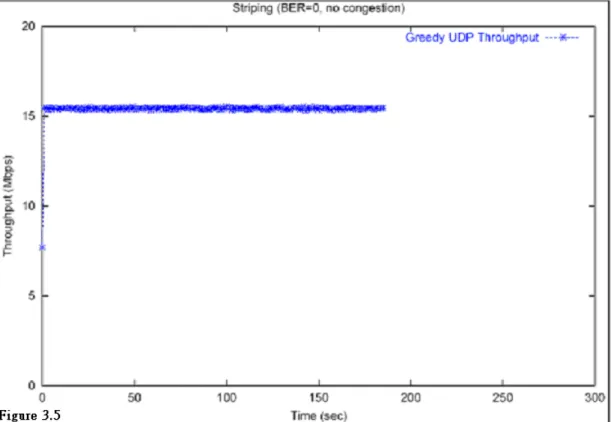
In addition to the performance of TCP traffic, we also did another simulation to evaluate the performance of UDP traffic. The scenario is the same as that for TCP except that we use the ttcp program to generate UDP traffic. Figure 3.5 shows the result. The speed-up is also almost three times.
3.2.1.1 Congestion
Now we add the factor of congestion in the simulation environment. Starting with a simple case, figure 3.6 shows the scenario. In Figure 3.6, Node 3 is in the transmission range of Node 1 and Node 2. So is Node 4. Notice that the wireless adaptors of Node 3 and Node 4 are configured to use channel 1. One of the striping adaptors of Node 1 and Node 2 are also configured to use channel 1. These four wireless adaptors share the same medium. If the transmissions of two pair of nodes, (Node1, Node2) and (Node3, Node4), run simultaneously, throughput will be only one half of the original throughput.
Figure 3.7 shows the result of throughput. As we can see, throughput of non-striping between node 3 and node 4 is 2.5 Mbps, half of the original throughput, because of medium sharing. Throughput of striping between node 1 and node 2 is about 12.5 Mbps. The wireless adaptors configured to use channel 1 can only get a throughput of 2.5 Mbps. The others adaptors can get full throughput of 5 Mbps since they don’t use channel 1. Thus the accumulated throughput is 12.5Mbps (2.5 + 5 + 5). This is the maximal aggregated throughput that can be
possibly archived. Here we can see that our striping algorithm can get good performance even under the situation of congestion. We use the same scenario for simulation but use the Surplus Round Robin. Figure 3.8 shows the result.
We add more nodes to test our striping algorithm. Figure 3.8 shows the scenario which contains 6 nodes. Node 5 and Node 6 are added and their wireless adaptors are configured to use channel 5. Figure 3.9 shows results of throughput. In this scenario, two striping adaptors in both Node 1 and Node 2 share the medium with others. Thus accumulated throughput is about 10Mbps (2.5 + 2.5 + 5).
Figure 3.10 shows another scenario which contains 8 nodes. Node 7 and Node 8 are added and their wireless adaptors are configured to use channel 9. Figure 3.11 shows result of throughput. All striping adaptors in both Node 1 and Node 2 share the medium with others. Thus accumulated throughput is about 7.5Mbps (2.5 + 2.5 + 2.5).
To see the performance of the Surplus Round Robin, we used the scenario in Figure 3.6 to run the simulation. Figure 3.12 shows the result. We can observe that performance is worse because congestion will cause more out-of-order packets.
These results show that our string algorithm can get a maximum aggregated throughput even under the situation of congestion.
3.2.1.2 Packet Error
In the above scenario, we assume that there is no packet error. The packet transmission is thus error-free. In the real world, this is impractical. Currently most of IEEE 802.11 wireless network products declare that there is a non-zero BER (bit error rate) which is less that 0.00001. Next we use a variety of BER values to run the simulations.
Again, in order to evaluate our striping algorithm, we run some simulations of non-striping in which BER is not zero. Figure 3.13 shows the results. We can see from figure 3.13 that throughput is a little lower when BER is not zero. Throughput is 4.1Mpbs, 4.5Mpbs, and 4.9Mbps when BER is 0.00001, 0.000005, and 0.000001 respectively.
Again we use the scenario in Figure 3.1 to run the striping simulations. But this time BER is set to a non-zero value. Figure 3.14 shows the results. Throughput is 12Mbps, 13.5Mbps, and 14.7Mpbs when BER is 0.00001, 0.000005, and 0.000001 respectively. They are the maximum aggregated throughput that can be achieved. The speed-up is also about three times. Figure 3.15 shows the results of the Surplus Round Robin. Again, we can observe that performance is worse because of packet errors.
In the each of above simulation cases, BER of all striping wireless adaptors of Node 1 and Node 2 is set to the same value. For example, we set BER of all adaptors to 0.00001 and get throughput of 12Mpbs. Figure 3.16 shows another scenario in which BER of each adaptor is different. Figure 3.17 shows the result. Throughput is about 13.4Mpbs. It is the accumulated result of three adaptors (4 + 4.5 + 4.9).
From these simulations, we can see that our striping algorithm can work well even under the situation of packet-error.
3.2.1.4 Other Issues
Mobility and the hidden terminal problem are common issues discussed in wireless network. We did two simulations about these to see the performance of our striping algorithm.
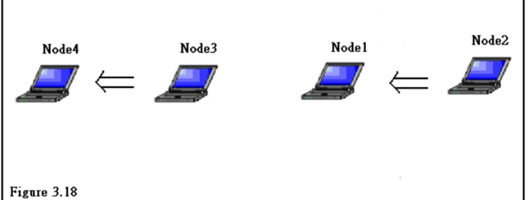
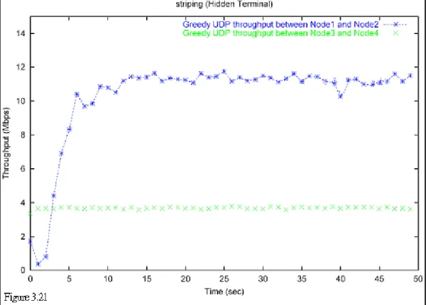
Figure 3.18 shows a scenario which has the hidden terminal problem. Node 1 is in the transmission ranges of both Node 2 and Node 3. But Node 2 is not in the transmission range of Node 3. Neither is Node3. Thus there is a hidden terminal problem here.
At first we didn’t use striping. Each of four nodes has only one wireless interfaces. Figure 3.19 shows the result. As we can see from the figure, transmission between Node 1 and Node 2 only gets throughput of 0.3 Mbps.
Then we apply striping on both Node 1 and Node 2. Figure 3.20 shows the result of using the Surplus Round Robin. Figure 3.21 shows the result of using our striping algorithm. We can see that we can get a maximum aggregated throughput (0.3 Mbps + 5 Mbps + 5 Mbps = 10.3 Mbps) by using our striping algorithm.
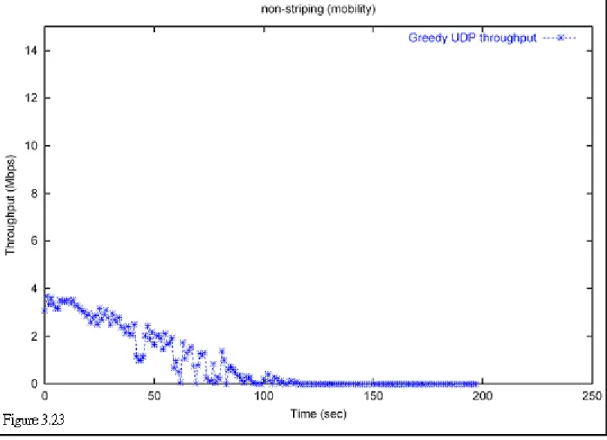
Figure 3.22 shows the next simulation scenario. Both Node 1 and Node 2 move with a speed of 0.7 m/s. Node 2 will transmit data to Node 1.
Again, we didn’t use striping at first. Figure 3.23 shows the result. Throughput is getting down as the distance between two nodes increases. When the distance exceeds the transmission range, the throughput becomes 0 Mbps.
Figure 3.24 shows the result of using the Surplus Round Robin. Figure 3.25 shows the result of using our striping algorithm. Throughput is also getting down as the distance increases. But our striping algorithm performs better than the Surplus Round Robin. A maximum aggregated
throughput, about 3 times of original throughput, still can be achieved.
3.2.1.3 Discussions
We can see that our striping algorithm can get the maximum aggregated throughput that can be achieved. The algorithm can also work well under the situation of congestion, packet-error, and mobility. Under these situations, skew must happen more frequently. Thus the reordering timer’s value must be set to a larger value to solve the problem of skew. Because the reordering timer is adjusted dynamically, the algorithm can get good performance results under situations of any degree of congestion or packet-error.
We can also see that the Surplus Round Robin doesn’t perform well. It cannot get the maximum aggregated throughput. Besides, because it doesn’t provide real FIFO, its TCP performance is bad and unstable.
3.2.2 Scalability Issue
The next simulation we did is to expand the number of striping wireless adaptors. In the above simulations, we use only three wireless adaptors for striping. We still use the basic scenario described in Figure 3.1 and use the stcp/rtcp program to generate traffic. We expand the adaptors’ number from three to ten. On each host, all adaptors are configured to use different frequency channels. For example, when we use ten wireless adaptors for striping, we configure them to use frequency channel 1 to 10, respectively. In the real world, using successive frequency channels may cause some interference. However in our simulation, we assume that there is no such interference. Figure 3.26 shows the result. We can see that the maximum aggregated throughput can be obtained while the number of striping adaptors is increased. This shows the scalability of our striping algorithm.
Latency is also an important metric to evaluate our striping algorithm. Since we set a reordering timer to reorder out-of-order packets, latency of a transmission will thus increase. We used the same simulation scenarios again to study latency issues. Here we didn’t use the stcp/rtcp programs to generate traffics. Instead, we used the stg/rtg programs, which are contained in the NCTUns 1.0 package, to generate UDP traffics. The rtg program will report latency of transmissions.
Latency (sec) Number of stripes
min max avg Stdev
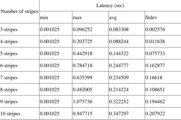
3 stripes 0.001025 0.096252 0.083308 0.002576 4 stripes 0.001025 0.203725 0.088244 0.011838 5 stripes 0.001025 0.442918 0.144322 0.075733 6 stripes 0.001025 0.784718 0.244777 0.162877 7 stripes 0.001025 0.635399 0.234509 0.16618 8 stripes 0.001025 0.482005 0.214224 0.108651 9 stripes 0.001025 1.075736 0.322252 0.194462 10 stripes 0.001025 0.947715 0.347297 0.207922 Table 3.1
Table 3.1 shows the results of simulation with different numbers of stripes. In the table, the first column lists the number of used stripes. The other columns list the minimum latency, the maximum latency, the average latency, and the standard deviation, respectively. As we can see, latency increases as we expand the number of stripes. This is because the possibility of receiving out-of-order packets increases while more stripes are used. When more stripes are used, packets are multiplexed over more stripes. Packets are thus more likely to be received out of order. This will cause the reordering timer to be increased. This in turn will cause latency to increase.
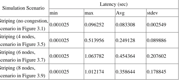
Latency (sec) Simulation Scenario
min max Avg stdev
Striping (no congestion,
scenario in Figure 3.1) 0.001025 0.096252 0.083308 0.002549 Striping (4 nodes, scenario in Figure 3.5) 0.001025 0.513956 0.249128 0.089886 Striping (6 nodes, scenario in Figure 3.7) 0.001025 1.063782 0.454364 0.207602 Striping (8 nodes, scenario in Figure 3.9) 0.001025 1.012174 0.358644 0.178845 Table 3.2
Table 3.2 shows the results of simulations with congestion. The first column lists simulation scenarios. The other columns list different kinds of latency. We can see that latency increases when the degree of congestion increases. The value of the reordering timer will certainly be increased because of congestion, which will in turn increase latency. Besides, when more adaptors are involved in congestion, it is more possible that packets are sent out of order because latency of each congestion stripe differs from each other.
Latency (sec) BER
min Max avg stdev
0.0 0.001025 0.096252 0.083308 0.002549 0.000001 0.001025 0.133014 0.086926 0.004745 0.000005 0.001025 0.256145 0.110644 0.026783 0.00001 0.001025 0.669147 0.177871 0.102995 Table 3.3
Table 3.3 shows the results of scenario with packet-error. We use three stripes and set the BER to different non-zero values. Latency increases when the value of BER increases. This is also because the value of the reordering timer increases. Higher value of BER causes more packets to be dropped. Thus the reordering timer is increased to wait for retransmission.
From these results, we know that we make a little sacrifice in latency to obtain higher aggregated bandwidth. The reordering timer can help keeping the FIFO delivery. But it also brings us longer transmission delays.
3.2.4 Reordering Timer Issue
The reordering timer plays a very important role in our striping algorithm. In order to observe its value, we did the following simulation. Figure 3.27 shows the scenario. During the first 50 seconds, there are three pairs of stcp/rtcp programs running simultaneously. During the second 50 seconds, there are only two pairs. Then there is only one pair running at last. The degree of congestion decreases as time proceeds. Figure 3.28 shows the value of the reordering timer obtained from Node 1.
there are three pairs of stcp/rtcp programs running at beginning, Node 1 will receive out-of-order packets because of congestion and increase the value of the reordering timer. Later when the adjusting timer is expired, the value of the reordering timer is halved. If there is still congestion, out-of-order packets will be received and the reordering timer will be increased again. As time proceeds, the degree of congestion will decrease, and Node 1 will not receive too many out-of-order packets. Then the value of the reordering timer will hold a stable value.
The result shows that the reordering timer is adjusted dynamically. The striping algorithm adjusts it according to the current environment. If a network is busy, the value of the reordering timer will be set to a higher value. If a network is idle, it will be set to a lower value. If a network is stable, it will be set to a stable value.
We did some simulations to evaluate performance of our striping algorithm. We can see that our striping algorithm can obtain the maximum aggregated throughput from simulation results. We also add the factors of packet-error and congestion in simulations. Simulation results show the flexibility of our striping algorithm. Even under the environment with lots of packet dropping (caused by congestion or packet-error), our striping algorithm can still obtain the maximum throughput.
To show the scalability of our striping algorithm, we expanded the number of striping wireless adaptors and did a series of simulations. The results show that our algorithm can still obtain the maximum aggregated throughput. Higher bandwidth can be obtained simply by expanding the number of striping wireless adaptors. However, latency will also increase when the number of adaptors increased.
We also did simulations to observe the latency. Since we use the reordering timer to delay the delivery of out-of-order packets, the latency will thus be a little longer. Besides, the bad network environment such as congestion or packet-error will cause latency to increase as well.
At last we did a simulation to observe the value of the reordering timer’s value. The value of the reordering timer changed dynamically. Based on the current network environment, it will be set to a proper value. In addition, if the current network environment is stable, it will be held in a stable state.
Chapter 4 Concluding Remarks
A striping algorithm based on the round robin scheme is proposed to aggregate multiple IEEE 802.11 wireless adaptors to gain higher bandwidth. This striping algorithm uses sequence numbers embedded in the packets to keep the FIFO delivery. A reordering-timer mechanism in the algorithm is used to queue out-of-order packets and reorder them. This can eliminate the triggering of TCP fast retransmit and thus avoid slowing down a TCP connection’s transfer progress. A mechanism of load balancing is used to route traffic to other stripes whose loads are lower.
We used the network simulation program, NCTUns 1.0, to evaluate the performance of our striping algorithm. NCTUns 1.0 uses the network subsystem of real-world FreeBSD and can thus generate more accurate simulation results. We conducted several experiments to evaluate the performance. As shown in the results, the aggregate throughput is the summation of throughput of individual adaptors. In addition, the striping algorithm can also perform well under the situation of packet-error and congestion.
By aggregating multiple wireless adaptors, users can obtain higher bandwidth to run network applications. Thus network applications that originally run on fixed networks and demand high bandwidth can also be run on mobile stations without the limitation of bandwidth. This is a low-cost and scalable way for achieving high wireless bandwidth.
References
[1] C. Brendan, S. Traw, and J. M. Smith. Striping within the network subsystem. IEEE Network, pages 22-29, July/August 1995.
[2] IEEE Std 802.11 Wireless LAN Medium Access Control (MAC) and Physical Layer (PHY) Specifications, June 1997.
[3] F. JACQUET, Philippe KAUFFMANN, Michel MISSON, Striping schemes for wireless communication system. The Fifth IEEE Symposium on Computer and Communications, Antibes, France, 4-6 July 2000
[4] F. JACQUET, Michel Misson, Striping over Wireless Links: Effects on Transmission Delays. [5] Hari Adiseshu, Guru Parulkar, and George Varghese, A reliable and scalable striping protocol. SIG-COMM, (8): 131-141, 1996.
[6] Jacob Jul Schroder, Design and Performance of Striping over ATM. Master’s thesis. February 1998.
[7] W. Richard Stevens, TCP/IP Illustrated, Volume1. Addison Wesley.
[8] S. Y. Wang and H. T. Kung, A Simple Methodology for Constructing Extensible and High-Fidelity TCP/IP Network Simulators. IEEE INFOCOM’99, March 21-25, 1999, New York, USA.
[9] S.Y. Wang, C.L. Chou, C.H. Huang, C.C. Hwang, Z.M. Yang, C.C. Chiou, C.C. Lin, The Design and Implementation of the NCTUns 1.0 Network Simulator. Computer Network Journals (to appear).
[10] C. H. Huang, The Design and Implementation of the NCTUns 1.0 Network Simulation Engine. Master’s thesis, National Chiao Tung University, Hsinchu, Taiwan, 2002.
可供推廣之研發成果資料表
R 可申請專利 □ 可技術移轉 日期:93 年 10 月 31 日國科會補助計畫
計畫名稱:使用 Wireless Trunks 來增加無線網路可用頻寬 計畫主持人: 王協源 計畫編號: 92-2213-E-009-063- 學門領域: 資訊技術/創作名稱
Wireless Trunks發明人/創作人
王協源 中文: 把數個網路介面卡聚合在一起形成一個單一對外的介面 (Trunk) ,由結合在一起的介面卡來提供累加的頻寬.這樣在上層 的應用程式看起來,就好像是頻寬增加了.這樣也就解決了頻寬不 足的間題.技術說明
英文:With currently available interface cards, we can aggregate them to get the accumulated bandwidth. In the applications’ view, they don’t know about what we do. They only feel that they have more bandwidth for use. This solves the problem of the bandwidth-shortage.