有限馬可夫鏈的對數索柏列夫常數

國

立

交

通

大

學

應用數學系

博

士

論

文

有限馬可夫鏈的對數索柏列夫常數

The Logarithmic Sobolev Constant on Finite Markov Chains

研 究 生：陳冠宇

指導教授：許元春

有限馬可夫鏈的對數索柏列夫常數

The Logarithmic Sobolev Constant on Finite Markov Chains

研 究 生：陳冠宇 Student：Guan-Yu Chen

指導教授：許元春 Advisor：Yuan-Chung Sheu

國 立 交 通 大 學

應 用 數 學 系

博 士 論 文

Submitted to Department of Applied Mathematics College of Science

National Chiao Tung University in partial Fulfillment of the Requirements

for the Degree of Doctor of Philosophy

in

Applied Mathematics

August 2006

Hsinchu, Taiwan, Republic of China

有限馬可夫鏈的對數索柏列夫常數

學生：陳冠宇

指導教授

許元春 教授

國立交通大學應用數學系博士班

摘

要

一副撲克牌要洗牌幾次其機率分佈才會接近均勻分佈。數學上，這個

問題是屬於有限馬可夫鏈收斂速度的計量分析。在其他的領域裡也有相似

的問題，其中包含了統計物理學、計算機科學和生物學。在這篇論文裡，

我們討論l

_{距離和超皺縮性之間的關係，並介紹兩個與收斂速度相關的常}

數－譜間隙和對數索柏列夫常數。

我們的目標是要準確地計算出對數索柏列夫常數，其中最主要的結果

就是在循環體上簡單隨機運動的對數索柏列夫常數。另外，透過馬可夫鏈

的崩塌，我們也得到兩種在直線上隨機運動的對數索柏列夫常數。最後，

我們考慮狀態空間為三個點的馬可夫鏈並求得部分的對數索柏列夫常數。

The Logarithmic Sobolev Constant on Finite Markov Chains

Student：Guan-Yu Chen

Advisors：Dr. Yuan-Chung Sheu

Department of Applied Mathematics

National Chiao Tung University

ABSTRACT

How many times a deck of cards needed to be shuffled in order to get close

to the uniform distribution. Mathematically, this question falls in the realm of

the quantitative study of the convergence of finite Markov chains. Similar

convergence rate questions for finite Markov chains are important in many

fields including statistical physics, computer science, biology and more. In this

dissertation, we discuss the relation between the l

-distance and the

hypercontractivity. To bound the convergence rate, we introduced two

well-known constants, the spectral gap and the logarithmic Sobolev constant.

Our goal is to compute the logarithmic Sobolev constant for nontrivial

models. Diverse tricks in use include the comparison technique and the collapse

of Markov chains. One of the main work concerns the simple random walk on

the n cycle. For n even, the obtained logarithmic Sobolev constant is equal to

half the spectral gap. For n odd, the ratio between the logarithmic Sobolev

constant and the spectral gap is not uniform.

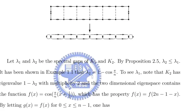
Ideally, if the collapse of a chain preserves the spectral gap and the original

chain has the logarithmic Sobolev constant equal to a half of the spectral gap,

then the logarithmic Sobolev constant of the collapsed chain is known and equal

to half the spectral gap. We successfully apply this idea to collapsing even

cycles to two different sticks. Throughout this thesis, examples are introduced to

illustrate theoretical results. In the last section, we study some three-point

Markov chains with introduced techniques.

誌

謝

首先我要感謝我的指導老師、同時也是我的精神導師許元春教授。在

他熱情和耐心的指導下，我在學術上的專業知識和論文寫作都有明顯的進

步。其次我要感謝每位博士學位口試委員在口試時給予的寶貴意見，以及

交大應用數學系每位老師的指導與教誨。

另外我要感謝長久以來一直支持我的親朋好友。因為他們的鼓勵，讓

我有更大的動力去完成博士學位。其中我要特別感謝我的父母親，他們在

經濟上的自主讓我能無後顧之憂的專心致力於學業。我要感謝我的兩個弟

弟，他們孜孜不倦的向學精神是我在研究遭遇瓶頸時的最大鼓勵。最後，

我要感謝敏玉--我的太太。因為她的陪伴與分享，我得以在平凡的日子裡

找到自己的興趣並預見未來努力的方向。

目

錄

中文摘要

……….

_i

英文摘要

……….

_ii

誌謝

……….

_iii

目錄

……….

_iv

1 Introduction

………

1

1.1

Preliminaries …..……….

2

1.2

The l

-distance and the submultiplicativity ………

10

1.3

Poincaré inequality and the spectral gap ………

10

2

Hypercontractivity and the logarithmic Sobolev constant .…

24

2.1

The logarithmic Sobolev constant ………..………

24

2.2 Hypercontractivity

……..………

28

2.3

Tools to compute the logarithmic Sobolev constant ………..

32

2.4

Some examples ...………

41

3

Logarithmic Sobolev constants for some finite Markov chains

48

3.1

The simple random walk on an even cycle ……….

48

3.1.1

The main result ………

49

3.1.2

Proof of Theorem 3.1 ..………

53

3.1.3

An application: Collapsing cycles and product of sticks…….

61

3.2

The simple random walk on the 5-cycle ..………...

65

3.3

Some other 3-point chains ………..………

70

Appendix A Techniques and proofs ………

79

A.1

Fundamental results of analysis ………..………

79

參考文獻

……….

₈₀

Chapter 1

Introduction

How many times a deck of cards needed to be shuffled in order to get close to the uniform distribution. Mathematically, this question falls in the realm of the quantitative study of the convergence of finite Markov chains. Similar convergence rate questions for finite Markov chains are important in many fields including statistical physics, computer science, biology and more. Many questions posted in these fields are to estimate the average of a function f defined on a finite set Ω with respect to a probability measure π on Ω. From the view point of Markov Chain Monte Carlo method, this is achieved by simulating a Markov chains with limiting distribution π and selecting a state at a random time T as a random sample. Knowing the qualitative behavior of convergence is not enough to determine the sampling time T . A quantitative understanding of the mixing time is essential for theoretical results. In practice, various heuristics are used to choose T .

Diverse techniques have been introduced to estimate the mixing time. Coupling and strong uniform time are discussed by Aldous and Diaconis in [1, 2]. Jerrum and Sinclair use conductance to bound mixing time in [17]. Application of rep-resentation theory appears in [8] and Diaconis and Saloff-Coste used comparison techniques in [9, 10]. For lower bound, important techniques are described in [7] and in more recent work of Wilson [27].

In this dissertation, we introduce two well-known constants, the spectral gap and the logarithmic Sobolev constant. Applying fundamental result in calculus and linear algebra, we are able to determine both constants for some specific models.

1.1

Preliminaries

Let X be a finite set. A discrete time Markov chain is a sequence of X -valued random variables (Xn)∞0 satisfying

P{Xn+1 = xn+1|Xi = xi, ∀0 ≤ i ≤ n} = P{Xn+1 = xn+1|Xn= xn}

for all xi ∈ X with 0 ≤ i ≤ n and n ≥ 0. A Markov chain is time homogeneous if

the quantity in the right hand side of the above identity is independent of n. In this case, such a Markov chains is specified by the initial distribution (the distribution of X0) and the one-step transition kernel K : X ×X → [0, 1](also called the Markov

kernel) which is defined by

∀x, y ∈ X , K(x, y) = P{Xn+1 = y|Xn= x}.

An immediate observation on the Markov kernel K is that P_y∈XK(x, y) = 1 for

all x ∈ X . Throughout this thesis, all Markov chains are assumed to be time homogeneous. For any Markov chain (Xn)∞0 with transition matrix K and initial

distribution µ, that is, P{X0 = x} = µ(x) for all x ∈ X , the distribution of Xn is

given by

∀x ∈ X , P{Xn= x} = (µKn)(x) =

X

y∈X

µ(y)Kn_{(y, x),}

where Kn _{is a matrix defined iteratively by}

∀x, y ∈ X , Kn_{(x, y) =}X z∈X

Kn−1_{(x, z)K(z, y).}

In a similar way, one may also consider a continuous-time Markov process. Here we consider only the following specific type. For any Markov kernel K, let (Xt)t≥0 be a Markov process with infinitesimal generator K − I(the Q-matrix

defined in [19]). One way to realize this process is to stay in a state for an ex-ponential(1) time and then move to another state according to the Markov kernel

K. In other words, the law of Xt is determined by the initial distribution µ

and the continuous-time semigroup Ht = e−t(I−K)(a matrix defined formally by

Ht(x, y) = e−t

P_∞

n=0t

n

n!Kn(x, y) for x, y ∈ X and t ≥ 0, where K0 = I) through

the following formula

∀x ∈ X , t ≥ 0, P{Xt = x} =

X

y∈X

µ(y)Ht(y, x).

Note that if (Yn)∞0 is a Markov chain with transition matrix K and Ntis a

Pois-son process with intensity 1 and independent of (Yn)∞0 , then the Markov process

(Xt)t≥0 with infinitesimal generator K − I satisfies Xt = Yd Nt(in distribution) for

t ≥ 0. This is because

∀x, y ∈ X , Ht(x, y) = E[KNt(x, y)] = P{YNt = y|Y0 = x}.

For any finite Markov process (Yt)t≥0, we may find a constant c > 0, a Markov

chain (Xn)∞1 and a Poisson(1) process independent of (Xn)∞1 such that Yt= XNct

in distribution, or equivalently

P{Yt= y|Y0 = x} = e−ct(I−K)(x, y), ∀x, y ∈ X ,

where K is the Markov kernel of (Xn)∞1 . To see the details, let Q be the

infinites-imal generator of (Yt)t≥0, which is a |X | × |X | matrix satisfying

Q(x, y) ≥ 0, ∀x 6= y, x, y ∈ X ,

and

X

y∈X

Q(x, y) = 0, ∀x ∈ X .

Then, for t ≥ 0, the law of Yt is given by

P{Yt = y|Y0 = x} = etQ(x, y) = ∞ X n=0 tn_Qn_{(x, y)} n! .

By letting q = max{−Q(x, x) : x ∈ X }, where we assume its positivity, and

K = q−1_{Q + I, one may check K(x, y) ≥ 0 and} P

yK(x, y) = 1 for all x, y ∈ X .

Then the distribution of Yt starting from x can be expressed by

P{Yt= y|Y0 = x} = etQ(x, y) = e−(tq)(I−K)(x, y), ∀x, y ∈ X .

Another view point on the continuous-time semigroup Ht is the following. For

any Markov kernel K, let L = LK be a linear operator on R|X | defined by

∀x ∈ X , Lf (x) = (K − I)f (x) =X

y∈X

K(x, y)f (y) − f (x). (1.1) The operator L can be viewed intuitively as a Laplacian operator on X . A di-rect computation shows that, for any real-valued function f on X , the function

u(t, x) = Htf (x) is a solution for the initial value problem of the discrete-version

heat equation, i.e.,      (∂t+ L)u = 0 u : R+× X → R u(0, x) = f (x) ∀x ∈ X .

For any Markov kernel K, a measure π on X is called invariant(with respect to K) if πK = π or equivalently

∀x ∈ X , X

y∈X

π(y)K(y, x) = π(x). (1.2) A measure π on X is called reversible if the following identity holds

∀x, y ∈ X , π(x)K(x, y) = π(y)K(y, x).

In this case, K is said to be reversible with respect to π. From these definitions, it is obvious that a reversible measure is an invariant measure. Besides, if π is invariant(resp. reversible) with respect to K, then, for all t ≥ 0, πHt = π

or equivalently P_y∈X π(y)Ht(y, x) = π(x) for all x ∈ X (resp. π(x)Ht(x, y) =

π(y)Ht(y, x) for all x, y ∈ X ).

Note that, for any Markov kernel K on X , a constant vector on X is a right eigenvector of K with eigenvalue 1. This implies the existence of a real-valued function f on X satisfying f = f K, or equivalently f (x) =P_yf (y)K(y, x) for all x ∈ X . By the following computation,

X x∈X |f (x)| =X x∈X ¯ ¯ ¯ ¯ ¯ X y∈X f (y)K(y, x) ¯ ¯ ¯ ¯ ¯≤ X x,y∈X |f (y)|K(y, x) =X y∈X |f (y)|,

one can find that |f | is also a left eigenvector of K with eigenvalue 1. Hence, for any Markov kernel, there exists a probability measure π, which is invariant with respect to K. In that case, π is called a stationary distribution for K.

A Markov kernel K is called irreducible if, for any x, y ∈ X , there exists n =

n(x, y) such that Kn_{(x, y) > 0. A state x ∈ X is called aperiodic if K}n_{(x, x) > 0}

for sufficiently large n, and K is called aperiodic if all states are aperiodic. It is known that under the assumption of irreducibility of K, there exists a unique stationary distribution π. In particular, the distribution π is positive everywhere. In addition, if K is irreducible, then K is aperiodic if and only if X has an aperiodic state.

Proposition 1.1. Let K be an irreducible Markov kernel on a finite set X with

the stationary distribution π. Then ∀x, y ∈ X , lim

t→∞Ht(x, y) = π(y).

If K is irreducible and aperiodic, then ∀x, y ∈ X , lim

n→∞K

Under mild assumptions —irreducibility for continuous-time Markov processes and irreducibility and aperiodicity for discrete-time Markov chains— Proposition 1.1 shows the qualitative result that Markov chains converge to their stationarity as time tends to infinity. If such a convergence happens, the Markov kernel is called ergodic.

Note that the irreducibility of a Markov chain is sufficient, by Proposition 1.1, but not necessary for the ergodicity. A counterexample for the necessity is to consider a Markov chain on a two point space {0, 1} whose kernel is given by

K(0, 0) = 1, K(0, 1) = 0, K(1, 0) = 1 − p, K(1, 1) = p,

where p ∈ (0, 1). In this example, K is not irreducible because Kn_{(0, 1) = 0 for}

n ≥ 0. A few computations show that for n ≥ 1 and t > 0, Kn₌    1 0 1 − pn _pn    , Ht=    1 0 1 − e(p−1)t _e(p−1)t    .

By the above formulas, the distribution of the Markov chain starting from any fixed state converges to (1, 0).

Proposition 1.2. Let K be a Markov kernel on a finite set X and π is a positive

probability measure on X . If, for all x, y ∈ X ,

lim

t→∞Ht(x, y) = π(y),

then K is irreducible. If the following holds

lim

n→∞K

n_{(x, y) = π(y), ∀x, y ∈ X ,}

By Proposition 1.1 and 1.2, if the limiting distribution is assumed positive, then, in continuous-time cases, K is ergodic if and only if K is irreducible, whereas, in discrete-time cases, ergodicity is equivalent to irreducibility and aperiodicity.

In many cases, the state space X is equipped with a group structure and the Markov kernel K is driven by a probability measure p on X in the following way.

K(x, y) = p(x−1y), ∀x, y ∈ X .

Let E be the support of p and, for n ≥ 1, En _{denote the set}

En = {x1x2· · · xn: xi ∈ E, ∀1 ≤ i ≤ n}.

In the above setting, it is clear that the irreducibility of K is equivalent to the existence of a positive integer n such that

X =

n

[

i=1

Ei.

Under the assumption of irreducibility of K, the Markov kernel K is aperiodic if and only if there exists a positive integer n such that X = En_.

The following proposition characterizes the irreducibility and the aperiodicity of finite Markov chains introduced in the previous paragraph, which has been proved many times by many authors. See [25, 26] for references.

Proposition 1.3 (Proposition 2.3 in [24]). Let X be a finite group and p be a

probability measure on X with support E = {x ∈ X : p(x) > 0}. Let K be a Markov kernel given by K(x, y) = p(x−1_{y) for x, y ∈ X . Then}

(1) K is irreducible if and only if E generates X , that is, any element of X can be expressed as a product of finitely many elements of E.

(2) Assume that K is irreducible. Then K is aperiodic if and only if E is not contained in a coset of any proper normal subgroup of X .

In particular, if X is simple and K is irreducible on X , then K is aperiodic.

To determine the reversibility of a Markov chain, by definition, one always needs to compute the stationary distribution first. In the following, we introduce a criterion to inspect the reversibility of a Markov chain without the computation of its stationary distribution.

Proposition 1.4. Let K be an irreducible Markov kernel on a finite set X with

stationary distribution π. Then (K, π) is reversible if and only if for any sequence {x0, ..., xn} with x0 = xn,

K(x0, x1)K(x1, x2) · · · K(xn−1, xn)

= K(xn, xn−1)K(xn−1, xn−2) · · · K(x1, x0).

(1.3)

Proof. Assume first that K is reversible with respect to π, that is, π(x)K(x, y) = π(y)K(y, x) for all x, y ∈ X . Let {x0, ..., xn} be a sequence with x0 = xn. Then

n−1 Y i=0 K(xi, xi+1) = n−1_Y i=0 π(xi+1)K(xi+1, xi) π(xi) = n−1_Y i=0 K(xi+1, xi).

For the other direction, we assume that (1.3) holds for any sequence {x0, ..., xn}

satisfying x0 = xn. This implies that for x, y ∈ X and n ≥ 1,

Kn(x, y)K(y, x) = X x1,...,xn−1 K(x, x1) n−2_Y i=1 K(xi, xi+1)K(xn−1, y)K(y, x) = X x1,...,xn−1 K(x, y)K(y, xn−1) n−2 Y i=1 K(xi+1, xi)K(x1, x) = K(x, y)Kn_{(y, x).}

Applying the above identity to the expansion formula of the continuous-time semi-group, we get

Letting t → ∞, the reversibility of K is then proved by Proposition 1.1.

The following is an application of the above proposition to random walks on finite trees.

Corollary 1.1. Let K be an irreducible Markov kernel on a finite set X and

G = (X , E) be an undirected graph induced from K whose vertex set is X and the edge set E is given by

E = {{x, y} ∈ X × X : x 6= y, K(x, y) + K(y, x) > 0}. If G is a tree, then K is reversible.

Remark 1.1. In Corollary 1.1, the induced graph G is connected if and only if K

is irreducible. In particular, if G is a tree, we have

∀x, y ∈ X , K(x, y) > 0 ⇐⇒ K(y, x) > 0.

Proof of Corollary 1.1. For convenience, any finite sequence of states in X is called

a path. For any path (x0, ..., xn), we let

Q_n−1

i=0 K(xi, xi+1) denote its “weight”. By

the above remark, it suffices to prove the identity (1.3) with paths of positive weight. To show this fact, we define D to be the set of all paths in G and, for all

x, y ∈ X , let f(x,y) be a function on D defined by

∀γ = (x0, ..., xn) ∈ D, f(x,y)(γ) =

n−1

X

i=0

δ(x,y)((xi, xi+1)) − δ(y,x)((xi, xi+1)).

Since G is a tree, it is obvious that, for all x, y ∈ X , f(x,y)(γ) ∈ {1, 0, −1} for any

positively weighted path γ ∈ D. If x0 = xn is assumed further, then f(x,y)(γ) = 0

for all x, y ∈ X . This implies that, for such a path γ, the multiplicity of the directed edge (x, y) in γ is the same as that of (y, x). Thus, for all x, y ∈ X , the multiplicity of (x, y) in γ is the same as that in the inverse path of γ, (xn, ..., x0),

1.2

The `

-distance and the submultiplicativity

As a consequence of Proposition 1.1, irreducible and aperiodic Markov chains con-verge in distribution to their stationarity. From the view point of the quantitative study, one may arise the following question: How fast the convergence can be? To answer this question, we need to specify the function used to measure the distance between the law of a Markov chain and its stationary distribution. In this section, we will introduce some frequently used distances or functions for measuring and give some basic results.

Definition 1.1. Let µ and ν be probability measures on a set X . The total

variation distance between µ and ν is denoted and defined by dTV(µ, ν) = kµ − νkTV= max

A⊂X{µ(A) − ν(A)}.

Let π be a positive probability measure on X . For 1 ≤ p ≤ ∞ and any (complex-valued) function f on X , the `p<sub>(π)-norm(or briefly the `</sub>p_{-norm) of f is}

defined by kf kp = kf k`p_(π) =        µ P x∈X |f (x)|p_π(x) ¶_1/p if 1 ≤ p < ∞ max x∈X |f (x)| if p = ∞ .

Definition 1.2. Let µ, ν and π be finite probability measures on X and assume that π is positive everywhere. The `p<sub>(π)-distance(or briefly the `</sub>p_-distance)

be-tween µ and ν is defined to be

dπ,p(µ, ν) = kf − gk`p_(π),

where f and g are densities of µ and ν with respect to π, that is, µ = f π and

Remark 1.2. From the above two definitions, it is easy to see that, for any

proba-bility measures µ and ν,

∀π > 0, dπ,1(µ, ν) = 2dTV(µ, ν).

Let (X , µ) be a measure space. It is well-known that, for 1 ≤ p ≤ ∞, if f is

`p_{-integrable, then} kf kp = sup kgkq≤1 Z X f (x)g(x)dµ(x),

where p−1 _{+ q}−1 _{= 1. By this fact, we may characterize the `}p_{-distance in the}

following way.

Proposition 1.5. Let π, µ, ν, f, g be the same as in Definition 1.2. Then, for 1 ≤ p ≤ ∞,

dπ,p(µ, ν) = sup khkq≤1

k(f − g)hk1,

where p−1_{+ q}−1 _{= 1.}

By Jensen’s inequality, if π is a positive probability measure, then

kf kp ≤ kf kq, ∀1 ≤ p < q ≤ ∞.

With this fact, we may compare the `p <sub>and `</sub>q _distances.

Proposition 1.6. Let π be a positive probability measure on X . For any two

probability measures µ, ν on X , one has

dπ,p(µ, ν) ≤ dπ,q(µ, ν), ∀1 ≤ p ≤ q ≤ ∞.

The following fact shows that, for fixed 1 ≤ p ≤ ∞, the `p_{-distance of Markov}

Proposition 1.7. Let K be an irreducible Markov kernel with stationary

distrib-ution π. Then, for 1 ≤ p ≤ ∞, the maps n 7→ max

x∈X dπ,p(K

n_{(x, ·), π) and t 7→ max}

x∈X dπ,p(Ht(x, ·), π)

are non-increasing and submultiplicative. In particular, if there exists β > 0 such that

max

x∈X dπ,p(K

m_{(x, ·), π) ≤ β (resp. max}

x∈X dπ,p(Hs(x, ·), π) ≤ β),

then for n ≥ m(resp. t ≥ s),

max

x∈X dπ,p(K

n_{(x, ·), π) ≤ β}bn/mc _{(resp. max}

x∈X dπ,p(Ht(x, ·), π) ≤ β bt/sc_).

Remark 1.3. By Proposition 1.7, if β ∈ (0, 1), then the exponential convergence of `p_{-distance has rate at least m}−1_{log(1/β) in discrete-time cases and rate s}−1_log(1/β)

in continuous-time cases.

For any Markov kernel K, we may associate it with a linear operator which is also denoted by K and defined by

Kf (x) =X

y∈X

K(x, y)f (y), ∀x ∈ X , f ∈ C|X |_.

In a similar way, we can view Ht and π as linear operators on C|X | by setting

Htf (x) = X y∈X Ht(x, y)f (y), π(f ) = X x∈X f (x)π(x).

To a standard usage, we let L∗ _{denote the adjoint operator of L. The}

follow-ing proposition equates the maximum `p_{-distance and the operator norm of the}

associated linear operator.

Proposition 1.8. Let K be an irreducible Markov operator with stationary

distri-bution π. For 1 ≤ p ≤ ∞,

max

x∈X dπ,p(K

n_{(x, ·), π) = kK}n_{− πk}

and

max

x∈X dπ,p(Ht(x, ·), π) = kHt− πkq→∞, for t ≥ 0,

where p−1_{+ q}−1 _{= 1 and for any linear operator L : `</sub>r<sub>(π) → `}s_(π),

kLkr→s= sup kf k`r (π)≤1

kLf k`s_(π). (1.4)

Remark 1.4. By Jensen’s inequality, for 1 ≤ p ≤ ∞, the linear operators Kn _and

Ht are contractions in `p, which means that

kKnkp→p ≤ 1, kHtkp→p ≤ 1.

This fact implies

kHt+s− πkp→∞≤ kHtkp→pkHs− πkp→∞≤ kHs− πkp→∞

and

kHt+s− πkp→∞≤ kHt− πkp→pkHs− πkp→∞

≤ kHt− πkp→∞kHs− πkp→∞.

By Proposition 1.8, these are the monotonicity and the submultiplicativity of the map t 7→ maxxdπ,q(Ht(x, ·), π), where p−1+ q−1 = 1. The same line of reasoning

also applies for the discrete-time cases.

Besides the `p_{-distance, there are many other functions of interest in measuring}

how close a Markov chain to its stationarity. We end this section by introducing two other well-known functions which are frequently used in probability theory and statistical physics. Let π be a positive probability measure on a finite set X . For any probability measure µ on X , let h be the density of µ with respect to π. The separation of µ with respect to π is defined by

dsep(µ, π) = max

and the (relative) entropy of µ with respect to π is defined by

dent(µ, π) = Entπ(µ) =

X

x∈X

[h(x) log h(x)]π(x).

(Generally, the entropy of any nonnegative function f on X with respect to any measure π is defined by Entπ(f ) = π[f log(f /π(f ))].) The following proposition

connects the `p_{-distance and the functions introduced above.}

Proposition 1.9. Let π and µ be probability measures on a finite set X and π is

positive everywhere. Then one has

1 2dπ,1(µ, π) ≤ dsep(µ, π) ≤ dπ,∞(µ, π) and 1 2dπ,1(µ, π) 2 _{≤ d} ent(µ, π) ≤ 1 2[dπ,1(µ, π) + dπ,2(µ, π) 2_].

Proof. Let h = µ/π. For the first part, it is obvious that maxx{1 − h(x)} ≤

kh − 1k∞. For the lower bound, setting A = {x ∈ X : h(x) < 1} implies that

max

x∈X{1 − h(x)} = maxx∈A{1 − h(x)} ≥

X

x∈A

{1 − h(x)}π(x) = kµ − πkTV.

For the second part, the upper bound is obtained by bounding the positive terms in the summation of the entropy though the following inequality.

∀u > 0, (1 + u) log(1 + u) ≤ u + u

2

2. For the lower bound, applying the fact

∀u > 0, √3|u − 1| ≤p(4u + 2)(u log u − u + 1) and Cauchy-Schwartz inequality implies that

As in Proposition 1.7, if the distance between a Markov chain and its station-arity is measured by the maximum separation and the maximum entropy, then it is decreasing in time.

Proposition 1.10. Let (X , K, π) be a finite Markov chain and Htbe the

continuous-time semigroup associated to K. Then the following maps n 7→ max x∈X dsep(K n_{(x, ·), π), t 7→ max} x∈X dsep(Ht(x, ·), π), (1.5) and n 7→ max x∈X dent(K n_{(x, ·), π), t 7→ max} x∈X dent(Ht(x, ·), π). (1.6)

are non-increasing. Furthermore, the maps in (1.5) are submultiplicative. Remark 1.5. By definition, if (X , K, π) an irreducible Markov chain, then

max

x∈X dsep(K(x, ·), π) = maxx∈X dsep(K

∗_{(x, ·), π).}

Proof of Proposition 1.10. Let A1 and A2 be two stochastic matrices satisfying

π = πA1 = πA2 and set A = A1A2. For the first part, it suffices to prove that

max

x∈X dsep(A(x, ·), π) ≤ maxx∈X dsep(A1(x, ·), π)

and

max

x∈X dent(A(x, ·), π) ≤ maxx∈X dent(A1(x, ·), π).

The first inequality can be easily obtained by the following computation. µ 1 −A(x, y) π(y) ¶ =X z∈X µ 1 −A1(x, z) π(z) ¶ µ π(z)A2(z, y) π(y) ¶ ≤ max z∈X ½ 1 − A1(x, z) π(z) ¾ , ∀x, y ∈ X .

For the second one, note that

∀x, y ∈ X , A(x, y) π(y) = X z∈X µ A1(x, z) π(z) ¶ µ π(z)A2(z, y) π(y) ¶ .

Since the function u 7→ u log u is convex, by Jensen’s inequality, one has A(x, y) π(y) log µ A(x, y) π(y) ¶ ≤X z∈X A1(x, z) π(z) log µ A1(x, z) π(z) ¶ π(z)A2(z, y) π(y) .

Multiplying π(y) on both sides, summing up all entries y in X and taking the maximum with respect to x implies the desired inequality.

For the submultiplicativity of the maximum separation, let A1, A2, A be the

same as in the previous paragraph. We prove this property by following the proof in [3]. Let c1 = maxxdsep(A1(x, ·), π) and c2 = maxxdsep(A2(x, ·), π). By definition,

we may express A1 and A2 as follows.

A1(x, y) = (1 − c1)π(y) + c1B1(x, y), ∀x, y ∈ X ,

and

A2(x, y) = (1 − c2)π(y) + c2B2(x, y), ∀x, y ∈ X ,

where B1 and B2 are stochastic matrices. Furthermore, one may check that πB1 =

πB2 = π. A simple calculation gives

A(x, y) =X z∈X A1(x, z)A2(z, y) = (1 − c1c2)π(y) + c1c2 X z∈X B1(x, y)B2(x, y) ≥ (1 − c1c2)π(y), ∀x, y ∈ X .

This proves the submultiplicativity of the maximum separation.

1.3

Poincar´

e inequality and the spectral gap

In this section, we introduce classical tools(the spectral gap of the transition ma-trix) to bound the `2_{-distance of continuous-time Markov chains to their stationary}

distributions. The following definition fits the classical notion of Dirichlet form if a Markov chain (X , K, π) is reversible.

Definition 1.3. Let (X , K, π) be an irreducible Markov chain. The quadratic form

E(f, g) = EK(f, g) = Reh(I − K)f, giπ, ∀f, g ∈ C|X |,

is called the Dirichlet form associated to the semigroup Ht = e−t(I−K), where h·, ·iπ

is the inner product in the complex space `2_(π).

By definition, if f = g, one can rewrite the Dirichlet form as follows.

Lemma 1.1. Let (X , K, π) be an irreducible Markov chain and E be the Dirichlet

form associated to the semigroup Ht. Then, for f ∈ C|X |,

E(f, f ) = h(I − 1 2(K + K ∗_{))f, f i} π = kf k22− RehKf, f iπ = 1 2 X x,y∈X |f (x) − f (y)|2K(x, y)π(x). In particular, one has

∂

∂tkHtf k

2

2 = −2E(Htf, Htf ), ∀t > 0. (1.7)

From (1.7), one can see that a bound of the ratio E(Htf, Htf )/kHtf k22 will give

a bound on the `2_{-norm of H}

tf . The following quantity is useful in bounding the

rate of the exponential convergence of the `2_-distance.

Definition 1.4. Let (X , K, π) be a Markov chain with Dirichlet form E. The spectral gap denoted by λ = λ(K) is defined by

λ = inf ½ E(f, f ) Varπ(f ) : Varπ(f ) 6= 0 ¾ ,

where Varπ(f ) is the variance of f , that is, Varπ(f ) = π(f − π(f ))2.

By definition, λ(K) = λ(K∗_{). Generally, the spectral gap is not an eigenvalue}

of I − K. Note that λ can be characterized by

If K is irreducible, the first equality in Lemma 1.1 and the minmax theorem in matrix analysis imply that the spectral gap is the smallest non-zero eigenvalue of

I − 1

2(K + K∗). In particular, if K is reversible, or equivalently, the operator K

is self-adjoint in `2_{(π), then λ is the smallest non-zero eigenvalue of I − K. Since}

the operator K + K∗ _{is self-adjoint, the spectral gap can be obtained by taking}

the infimum of the ratio in Definition 1.4 over all real-valued functions f .

Definition 1.5. Let (X , K, π) be an irreducible Markov chain. A Poincar´e in-equality is an inin-equality of the following type

kf − π(f )k2

2 ≤ CE(f, f ), ∀f ∈ `2(π),

where C is a positive constant in dependent of f .

From the above definition, if the Poincar´e inequality holds for a Markov kernel

K with constant C, then λ(K) ≥ C−1_{. In other words, the spectral gap is the}

inverse of the smallest C such that the Poincar´e inequality holds.

By applying (1.7), we may bound the operator norm kHt− πk2→2 from above

by using the spectral gap.

Proposition 1.11. Let (X , K, π) be an irreducible Markov chain and λ be the

spectral gap of K. Then the continuous-time semigroup Ht satisfies

∀f ∈ `2(π), kHtf − π(f )k22 ≤ e−2λtVarπ(f ).

Proof. Let g = f − π(f ). By Lemma 1.1, one has ∂

∂tkHtgk

2

2 = −2E(Htg, Htg) ≤ −2λVarπ(Htg) = −2kHtgk22.

This implies that

Remark 1.6. Since the Dirichlet form and the variance are invariant under the

addition of a constant vector, the conclusion in Proposition 1.11 is equivalent to saying that

kHt− πk2→2 ≤ e−λt, ∀t > 0.

By considering the spectrum of a Markov kernel, if K is reversible, we have kHt−

πk2→2 = e−λt for all t > 0. In general, this identity does not hold for all t > 0.

However, it is proved in [12] that λ is the largest value β such that kHt− πk2→2 ≤

e−βt _{for all t > 0.}

By Proposition 1.11, we may derive an upper bound on the `2_{-distance for}

continuous-time Markov chains.

Theorem 1.1. Let (X , K, π) be an irreducible Markov chain and λ be the spectral

gap of K. One has

∀x ∈ X , dπ,2(Ht(x, ·), π) ≤ π(x)−1/2e−λt, and ∀x, y ∈ X , |Ht(x, y) − π(y)| ≤ p π(y)/π(x)e−λt_. Proof. Let H∗

t be the adjoint operator of Ht and set δx(y) = π(x)−1 if x = y

and δx(y) = 0 otherwise. Since λ(K) = λ(K∗), we have, by letting f = δx in

Proposition 1.11,

dπ,2(Ht(x, ·), π)2 = kHt∗δx− π(δx)k22 ≤ e−2λtVarπ(δx) =

¡

π(x)−1− 1¢e−2λt.

This proves the first identity. For the second one, note that

This implies that, for x, y ∈ X , |Ht(x, t) − π(y)| = π(y) ¯ ¯ ¯ ¯ ¯ X z∈X µ Ht/2(x, z) π(z) − 1 ¶ Ã_H∗ t/2(y, z) π(z) − 1 ! π(z) ¯ ¯ ¯ ¯ ¯ ≤ π(y)dπ,2(Ht/2(x, ·), π)dπ,2(Ht/2∗ (y, ·), π) ≤pπ(y)/π(x)e−λt_,

where the first inequality applies the Cauchy-Schwartz inequality.

To relate the spectral gap and the spectrum of K, we define another quantity as follows.

ω = ω(K) = min{Reβ : β 6= 0, β is an eigenvalue of I − K}. (1.8) Since Ht = e−t(I−K), it follows that the spectral radius of Ht− π in `2(π) is e−tω.

This implies, for all 1 ≤ p ≤ ∞,

kHt− πkp→p ≥ e−ωt, ∀t > 0. (1.9)

In particular, we have, by applying the operator theory, lim

t→∞kHt− πk

1/t

p→q = e−ω, ∀1 ≤ p, q ≤ ∞.

The next theorem summarizes the above fact.

Theorem 1.2. Let (X , K, π) be an irreducible Markov chain, λ be the spectral gap

of K and ω be the quantity defined in (1.8). For all 1 ≤ p ≤ ∞,

lim t→∞ −1 t log µ max x∈X dπ,p(Ht(x, ·), π) ¶ = ω. In particular, λ ≤ ω.

Proof. Immediate from Proposition 1.8, Remark 1.6 and the discussion in the

As a consequence of Theorem 1.2, the rate of the exponential convergence of the maximum `p_{-distance is asymptotically ω, not the spectral gap λ. However, if}

an irreducible Markov kernel K is normal, that is, K∗_{K = KK}∗_{, then λ = ω. This}

implies that the asymptotical rate of the exponential convergence is the spectral gap. From this discussion, one can see that the spectral gap is closely related to the long-term behavior of a Markov chain. To reflect the finite-time behavior of the convergence and the notion of “time to equilibrium”, we consider the following quantity.

Definition 1.6. Let (X , K, π) be an irreducible Markov chain and Ht be the

associated continuous-time semigroup. For 1 ≤ p ≤ ∞, the `p_{-mixing time is}

denoted by Tp = Tp(K) and defined by

Tp = inf ½ t > 0 : max x∈X dπ,p(Ht(x, ·), π) ≤ 1/e ¾ .

By (1.9) and Theorem 1.1, we may bound the `p_{-mixing time as follows.}

Theorem 1.3. Let (X , K, π) be an irreducible Markov kernel and set π∗ = min{π(x) :

x ∈ X }. For 1 ≤ p ≤ 2, 1 ω ≤ Tp ≤ 1 λ µ 1 + 1 2log 1 π∗ ¶ , and, for 2 < p ≤ ∞, 1 ω ≤ Tp ≤ 1 λ µ 1 + log 1 π∗ ¶ .

Proof. The lower bound is obtained from (1.9) and Proposition 1.8. For the upper

bounds, note that, by Proposition 1.6, the identities in Theorem 1.1 imply that

∀1 ≤ p ≤ 2, max x∈X dπ,p(Ht(x, ·), π) ≤ π −1/2 ∗ e−λt and ∀1 ≤ p ≤ ∞, max x∈X dπ,p(Ht(x, ·), π) ≤ π −1 ∗ e−λt.

This is sufficient to prove the desired upper bounds.

For an illustration of the above theorem, we consider the following example.

Example 1.1. Fix n > 1 and let Kn be a Markov kernel given by

Kn(x, x + 1) = Kn(x, x − 1) = 1/2, ∀x ∈ Zn,

where Zn is the n-cycle. It is an easy exercise that Kn is irreducible and the

stationary distribution πn is a uniform distribution on Zn. By a method in Feller

[13, p.353], the following functions

φn,i(j) = cos(2πij/n), ∀0 ≤ j ≤ n − 1, 0 ≤ i ≤ b(n − 1)/2c,

and

φn,n−i(j) = sin(2πij/n), ∀0 ≤ j ≤ n − 1, 1 ≤ i ≤ d(n − 1)/2e,

are eigenfunctions of Kn and the corresponding eigenvalues βn,0, βn,1, ..., βn,n−1 are

given by

βn,0= 1, βn,i= βn,n−i = cos(2πi/n), ∀1 ≤ i ≤ d(n − 1)/2e.

Since Kn is reversible, the spectral gap is λ(Kn) = ω(Kn) = 1 − cos(2π/n).

Let Hn,t be the continuous-time semigroup associated to Kn. Applying

Theo-rem 1.1 and TheoTheo-rem 1.3 and using (1.9) derives

e−t(1−cos(2π/n))_{≤ d} π,2(Hn,t(x, ·), π) ≤ √ ne−t(1−cos(2π/n))_{, ∀n ≥ 1.} and, for 1 ≤ p ≤ ∞, n2 2π2 ∼ 1 1 − cos(2π/n) ≤ Tp(Kn) ≤ 1 1 − cos(2π/n)(1 + log n) ∼ n2_{log n} 2π2 .

This means that, for 1 ≤ p ≤ ∞, the `p_{-distance of continuous-time Markov chains}

after the time Cn2_{log n for large C. It is worthwhile noting that the correct order}

Chapter 2

Hypercontractivity and the logarithmic

Sobolev constant

Since Gross introduced the notions of the logarithmic Sobolev constant and of the hypercontractivity, many techniques are developed to compute the logarithmic Sobolev constant. The hypercontractivity is proved useful in bounding the conver-gence rate of Markov chains to their stationarity. An informative account of the development of logarithmic Sobolev inequalities can be found in the survey paper [14].

In Section 2.1, we define the logarithmic Sobolev constant and use it to bound the entropy of a Markov chain. In Section 2.2, we introduce how the hypercontrac-tivity can be used to bound the `p<sub>-distance and the `</sub>p_{-mixing time. In Section 2.3,}

diverse techniques for the estimation of the logarithmic Sobolev constant are intro-duced. In Section 2.4, we determine the explicit value of the logarithmic Sobolev constant for some examples.

2.1

The logarithmic Sobolev constant

The definition of the logarithmic Sobolev constant is very similar to that of the spectral gap. For a motive of why we concern such a constant, let’s start by looking at the relative entropy of the continuous-time Markov chain. Let (X , K, π) be an irreducible Markov chain, Ht be the associated continuous-time semigroup of K

with respect to π is defined by

Entπ(µ) = π(h log h),

where µ = hπ. Here we abuse the usage of Ent by letting Entπ(f ) = π(f log f ),

if f is a any nonnegative function but not a probability measure. A simple com-putation shows that, for any probability measure µ, P_xµ(x)/π(x) 6= 1 and

Entπ(µHt) = Entπ Ã X y∈X π(y)Ht(y, ·) π(·) µ(y) π(y) ! = Entπ(Ht∗h),

where h = µ/π. In the above setting, we have

∀t > 0, ∂

∂tEntπ(H

∗

th) = −E(Ht∗h, log(Ht∗h)) ≤ −2E(

p H∗ th, p H∗ th), (2.1)

where the inequality is proved by Diaconis and Saloff-Coste in [11, Lemma 2.7] and has an improved coefficient 4 instead of 2 if K is assumed reversible. By (2.1), one can see that a bound on the ratio Entπ(Ht∗h)/E(

p H∗ th, p H∗ th) suffices to give a

bound the rate of the convergence. To define the logarithmic Sobolev constant, we need to replace the variance by the following entropy-like quantity.

L(f ) = Lπ(f ) = X x∈X |f (x)|2_log µ |f (x)|2 kf k2 2 ¶ π(x). (2.2) Since u 7→ u log u is convex, Jensen’s inequality implies that L(f ) is nonnegative. Furthermore, if π is positive everywhere, then L(f ) = 0 if and only if f is constant. Note that if kf k2 = 1, that is, f2 is the probability density of µ = f2π with

respective to π, then

Definition 2.1. Let (X , K, π) be an irreducible Markov chain and L be the func-tional defined in (2.2). The logarithmic Sobolev constant α = α(K) is defined by α = inf ½ E(f, f ) L(f ) : L(f ) 6= 0 ¾ .

By definition, it is clear that α(K) = α(K∗_{). Obviously, one has L(f ) = L(|f |)}

and E(|f |, |f |) ≤ E(f, f ). By these facts, the logarithmic Sobolev constant can be obtained by taking the infimum of the ratio E(f, f )/L(f ) over all nonnegative functions f .

Definition 2.2. Let (X , K, π) be an irreducible Markov chain and E be the Dirich-let form. A logarithmic Sobolev inequality is an inequality of the following type.

CL(f ) ≤ E(f, f ), for all function f , where C is a nonnegative constant.

By the above definition, if the logarithmic Sobolev inequality holds for some constant C ≥ 0, then α ≥ C. In other words, α is the largest constant C such that the logarithmic Sobolev inequality holds. One may think of the existence of a function f such that the ratio E(f, f )/L(f ) is equal to 0, which means that the logarithmic Sobolev inequality never holds unless C = 0. It has been proved that the irreducibility eliminates such a possibility. Thus, one needs to consider only the case C > 0 in Definition 2.2. For a proof of the fact α > 0, please see Proposition 2.3. By (2.1), the entropy of a continuous-time Markov chain is bounded from above as follows.

Proposition 2.1. Let (X , K, π) be an irreducible Markov chain, Ht be the

measure on X . Then one has Entπ(µHt) ≤        e−2αt_Ent π(µ) in general e−4αt_Ent π(µ) if K is reversible. In particular, for x ∈ X , Entπ(Ht(x, ·)) ≤        e−2αt_log 1 π(x) in general e−4αt_log 1 π(x) if K is reversible.

Proof. Let h = µ/π. By (2.1), one can easily prove that for t > 0,

Entπ(µHt) = Entπ(Ht∗h) ≤ e−2αtEntπ(h) = Entπ(µ).

The same proof as above works for the reversible cases. The second part is followed by letting µ = δx, where δx(y) = 1 if y = x and δx(y) = 0 otherwise.

By applying Proposition 1.9 and Proposition 2.1, one may give an upper bound on the total variation distance.

Corollary 2.1. Let (X , K, π) be an irreducible Markov chain and α be the

loga-rithmic Sobolev constant of K. Then, for t > 0, dπ,1(Ht(x, ·), π) ≤ p 2 log(1/π(x))e−αt_, and, if K is reversible, dπ,1(Ht(x, ·), π) ≤ p 2 log(1/π(x))e−2αt_.

In particular, one has

T1 ≤ 1 2α µ 3 + log₊log 1 π∗ ¶ , and, for reversible chains,

T1 ≤ 1 4α µ 3 + log₊log 1 π∗ ¶ , where π∗ = minxπ(x) and log+t = max{0, log t}.

2.2

Hypercontractivity

In the previous section, the entropy and the `1_{-distance of a continuous-time}

Markov chain are proved to converge exponentially with rate at least the loga-rithmic Sobolev constant. It is natural to consider using the logaloga-rithmic Sobolev constant to bound the `p_{-distance. The following theorem is the well-known}

hy-percontractivity introduced in [14], which is sufficient to derive a bound on the

`p_-distance.

Theorem 2.1. (Theorem 3.5 in [11])Let (X , K, π) be an irreducible Markov

chain and α be the logarithmic Sobolev constant of K.

(1) Assume that there exists β > 0 such that kHtk2→q ≤ 1 for all t > 0 and

2 ≤ q < ∞ satisfying e4βt_{≥ q − 1. Then βL(f ) ≤ E(f, f ) for all f , and thus}

α ≥ β.

(2) Assume that (K, π) is reversible. Then kHtk2→q ≤ 1 for all t > 0 and

2 ≤ q < ∞ satisfying e4αt _{≥ q − 1.}

(3) For non-reversible chains, we have kHtk2→q ≤ 1 for all t > 0 and 2 ≤ q < ∞

satisfying e2αt _{≥ q − 1.}

Proof. See the proof given in [11].

Remark 2.1. Note that if (K, π) is reversible, then the first two assertions in

The-orem 2.1 characterize the logarithmic Sobolev constant as follows.

α = max{β : kHtk2→q ≤ 1, ∀t ≥ _4β1 log(q − 1), 2 ≤ q < ∞}.

To point out a surprising observation from the hypercontractivity, we recall the following fact in [23].

Lemma 2.1. Assume that K is a normal operator on `2_{(π) and β}

0 = 1, β1, ..., β|X |−1

are the eigenvalues of K with corresponding eigenvectors φ0 ≡ 1, φ1, ..., φ|X |−1.

Then, for all x ∈ X , one has

kHt(x, ·)/πk22 =

|X |−1_X i=0

e−2t(1−Reβi)_|φ

i(x)|2.

It follows from the above lemma that kHtk2→∞ > 1 if K is normal. Since

Ht is a contraction in `2 and has eigenvalue 1 with corresponding eigenvector 1,

we have kHtk2→2 = 1. A nontrivial observation, even in the discrete setting of a

state space, from the hypercontractivity is the existence of 0 < tq < ∞, for any

2 < q < ∞, such that kHtk2→q = 1 when t ≥ tq.

By Theorem 2.1, we may bound the `p_{-distance from above by using the}

loga-rithmic Sobolev constant.

Theorem 2.2. Let (X , K, π) be an irreducible Markov chain and λ and α be the

spectral gap and the logarithmic Sobolev constant of K. Then, for ², θ, σ ≥ 0 and t = ² + θ + σ, dπ,2(Ht(x, ·), π) ≤        kH²(x, ·)/πk2/(1+e 4αθ₎ 2 e−λσ if K is reversible kH²(x, ·)/πk2/(1+e 2αθ₎ 2 e−λσ in general . In particular, for c ≥ 0, one has

dπ,2(Ht(x, ·), π) ≤ e1−c, as t =        (4α)−1_log +log(1/π(x)) + cλ−1 if K is reversible (2α)−1_log +log(1/π(x)) + cλ−1 in general , where log₊t = max{0, log t}.

Proof. We consider only the reversible case by using Theorem 2.1(2), while the

general case can be proved by applying Theorem 2.1(3). Let θ > 0 and q(θ) = 1 + e4αθ_{. By Theorem 2.1(2), it is clear that kH}

θk2→q(θ) ≤ 1, and by the duality

given in Lemma A.1, it follows that kH∗

θkq0_(θ)→2 ≤ 1, where q(θ)−1+ (q0(θ))−1 = 1.

For convenience, let hx

t denote the density of Ht(x, ·) with respect to π. Note that

hx

t+s = Ht∗hxs. This implies

khx

t − 1k2 = k(Hσ∗− π)(Hθ∗hx²)k2

≤ kH_σ∗− πk2→2kHθ∗kq0_(θ)→2kh_²xk_q0_(θ)≤ e−λσkhx_²k2/q(θ)₂ ,

where the last inequality uses Remark 1.6 and the following H¨older inequality.

kf kq0 ≤ kf k1−2/q₁ kf k2/q₂ ,

for all 1 ≤ q0 _{≤ 2 and q}−1_{+ (q}0₎−1 _{= 1. This proves the first inequality.}

For the second part, note that khx

0k2 = π(x)−1/2 for x ∈ X . By letting ² = 0, we obtain khx_t − 1k2 ≤ µ 1 π(x) ¶_1/(1+e4αθ₎ e−λσ.

Let σ = cλ−1_{. To get the desired upper bound for the `}2_{-distance, we let σ = cλ}−1_,

choose θ = 0 if π(x) > e−1_{, and put}

θ = 1

4αlog log 1

π(x),

if π(x) < e−1_.

Using the Cauchy-Schwartz inequality, the `∞_{-distance can be bounded from}

above by the `2_{-distance. In fact, for t > 0, one has}

|ht(x, y) − 1| = ¯ ¯ ¯ ¯ ¯ X z∈X (ht/2(x, z) − 1)(h∗t/2(y, z) − 1)π(z) ¯ ¯ ¯ ¯ ¯ ≤ kht/2(x.·) − 1k2kh∗t/2(y, ·) − 1k2.

This implies the following corollary.

Corollary 2.2. Let (X , K, π) be an irreducible Markov chain and λ and α be the

spectral gap and logarithmic Sobolev constant of K. Then, for c > 0, one has |Ht(x, y)/π(y) − 1| ≤ e2−c, if t =        1 4α ³ log₊log 1

π(x)+ log+logπ(y)1

´ + cλ−1 _{if K is reversible} 1 2α ³ log₊log 1

π(x)+ log+logπ(y)1

´

+ cλ−1 _{in general}

, where log₊t = max{0, log t}.

Summing up Theorem 2.2 and Corollary 2.2, we may bound the `p_{-mixing time}

by using the logarithmic Sobolev constant.

Corollary 2.3. Let K be a reversible and irreducible Markov chain with stationary

distribution π and α be the logarithmic Sobolev constant. For 1 ≤ p ≤ ∞, let Tp

be the `p_{-mixing time of K. Then, for 1 < p ≤ 2,}

1 2mpα ≤ Tp ≤ 1 4α µ 4 + log₊log 1 π∗ ¶ and for 2 < p ≤ ∞, 1 2α ≤ Tp ≤ 1 2α µ 3 + log₊log 1 π∗ ¶

where log₊t = max{0, log t}, π∗ = minxπ(x) and mp = 1 + d(2 − p)/(2p − 2)e.

Proof. The upper bounds are obtained immediately from Theorem 2.2 and

Corol-lary 2.2. For the lower bound, Theorem 3.9 in [11] proves the case 2 < p ≤ ∞. For 1 < p ≤ 2, we use the fact

Remark 2.2. For general cases, Theorem 2.2 and Corollary 2.2 derive an upper

bound of the `p_{-mixing time which is twice of that in Corollary 2.3.}

Remark 2.3. Comparing Corollary 2.3 with Theorem 1.3, one may find that to

bound the `p_{-mixing time of a reversible continuous-time Markov chain, the}

loga-rithmic Sobolev constant is more closely related to Tp than the spectral gap.

2.3

Tools to compute the logarithmic Sobolev constant

It follows from Theorem 1.3 and Corollary 2.3 that the logarithmic Sobolev con-stant provides a tighter bound(in the sense of order) for the time to equilibrium

Tp than the spectral gap. Based on Corollary 2.3, to bound the `p-mixing time by

using the logarithmic Sobolev constant, we need to determine its value. For this view point, it is natural to ask: can one compute explicitly or estimate the con-stant α? In this section, we introduce several established tools to help determine the logarithmic Sobolev constant.

1. Bounding α from above by using the spectral gap λ. The following proposition establishes a relation between the spectral gap and the logarithmic Sobolev constant.

Proposition 2.2. (Lemma 2.2.2 in [23]) Let (X , K, π) be an irreducible Markov

chain. Then the spectral gap λ and the logarithmic Sobolev constant α of K satisfy α ≤ λ/2. Furthermore, let φ be an eigenvector of the matrix 1

2(K + K∗) whose

corresponding eigenvalue is (1 − λ). If π(φ3_{) 6= 0, then α < λ/2.}

Proof. We show by following the proof in [23] whose original idea comes from [22].

have f2log f2 = (1 + 2²g + ²2g2)¡2²g − ²2g2+ 2 3² 3_g3_{+ O(²}4₎¢ = 2²g + 3²2_g2₊ 2 3²3g3+ O(²4), and f2log kf k2₂ = (1 + 2²g + ²2g2)£2²π(g) + ²2(π(g2) − 2π(g)2) + ²3¡8 3π(g)3− 2π(g)π(g2) ¢ + O(²4₎¤ = 2²π(g) + ²2(4gπ(g) + π(g2) − 2π(g)2) + ²3£8 3π(g)3− 2π(g)π(g2) + 2gπ(g2) − 4gπ(g)2_{+ 2g}2_π(g)¤_{+ O(²}4₎ Thus, f2_log f2 kf k2 2 = 2² [g − π(g)] + ²2£_3g2_{− 4gπ(g) − π(g}2_{) + 2π(g)}2¤ + ²3£2 3g 3 ₋8 3π(g) 3_{+ 2π(g)π(g}2_{) − 2gπ(g}2₎ + 4gπ(g)2− 2g2π(g)¤+ O(²4) and L(f ) = 2²2_Var π(g) + ²3 £₂ 3π(g 3_{) +} 4 3π(g) 3_{− 2π(g)π(g}2₎¤_{+ O(²}4_),

where O(·) depends only on kgk∞.

To finish the proof, note that E(f, f ) = ²2_{E(g, g). Let φ be an eigenfunction}

of 1

2(K + K∗) whose eigenvalue is 1 − λ. By definition, it is clear that E(φ, φ) =

λVarπ(φ) and π(φ) = 0. Letting g = φ implies

α ≤ E(f, f ) L(f ) =

λVarπ(φ)

The first inequality is obtained by letting ² → 0. For the second part, since

π(φ3_{) 6= 0, we may choose |²| > 0 such that ²π(φ}3_{) > 0 and} 2

3²π(φ3) > O(²2). This

proves the second inequality.

2. One sufficient condition for α = λ/2. As a consequence of Proposition 2.2, the logarithmic Sobolev constant α is bounded from above by λ/2. Furthermore, a sufficient condition for the case 2α < λ is also given in that proposition. In the following, we give a necessary condition for the situation 2α < λ to happen. Proposition 2.3. (Theorem 2.2.3 in [23]) Let (X , K, π) be an irreducible

Markov chain and λ and α be the spectral gap and the logarithmic Sobolev con-stant of K. Then either α = λ/2 or there exists a positive non-concon-stant function u which is a solution of

2u log u − 2u log kuk2 =

1

α(I − K)u = 0, (2.3) where α = E(u, u)/L(u). In particular, α > 0.

Proof. We prove by considering the minimizer of the infimum in Definition 2.1.

Note that we may restrict ourselves to non-negative vectors with mean 1(under

π). By definition, either α is attained by a nonnegative non-constant vector, say u, or the infimum is attained at the constant vector 1. In the latter case, one may

choose a minimizing sequence (1 + ²ngn)∞1 satisfying

²n→ 0 and π(gn) = 0, kgnk2 = 1, ∀n ≥ 1.

This implies that the sequence {kgnk∞} is bounded from above and below by

positive numbers. Then, by the proof of Proposition 2.2, we get

α = lim n→∞ E(1 + ²ngn, 1 + ²ngn) L(1 + ²ngn) = lim n→∞ E(gn, gn) 2Varπ(gn) + O(²n) ≥ lim inf n→∞ λ 2 + O(²n) = λ 2

This proves α = λ/2.

If α is attained by a nonnegative non-constant vector f , then by viewing

E(f, f )/L(f ) as a function defined on R|X |_{, we have the following Euler-Lagrange}

equation ∇ µ E(f, f ) L(f ) ¶ ¯_¯ ¯ ¯ f =u = 0,

which is identical to (2.3). To show the positiveness of u, observe that if u(x) = 0 for some x ∈ X , then (2.3) implies that Ku(x) = 0, or equivalently, u(y) = 0 if

K(x, y) > 0. Thus, by the irreducibility of K, one has u ≡ 0, which contradicts

the assumption that u is not constant.

Remark 2.4. Note that a constant function is always a solution of (2.3).

Corollary 2.4. Let (X , K, π) be an irreducible Markov chain and λ and α be the

spectral gap and logarithmic Sobolev constant of K. If a non-constant function u on X and a positive number β satisfy the following system of equations

(I − K)u = 2β(u log u − u log kuk2), (2.4)

then β = E(u, u)/L(u). In particular, (2.4) has no non-constant solution for β ∈

(0, α). Moreover, if (2.4) has no non-constant solution for β ∈ (0, λ/2), then

α = λ/2.

3. Comparison technique. In many cases, the model of interest is complicated but can be replaced by a simpler one. In that case, the tradeoff of the replacement can be the loss of the accuracy of α(up to a constant) but the advantage is the simplicity of the new chain and, mostly, α is of the same order as the logarithmic Sobolev constant of the new Markov chain.

Proposition 2.4. (Lemma 2.2.12 in [23]) Let (X1, K1, π1) and (X2, K2, π2) be

irreducible Markov chains and E1 and E2 be respective Dirichlet forms. Assume

that there exists a linear map

T : `2(π1) → `2(π2)

and constant A > 0, B ≥ 0, a > 0 such that, for all f ∈ `2_(π 1),

E2(T f, T f ) ≤ AE1(f, f ), aVarπ1(f ) ≤ Varπ2(T f ) + BE1(f, f ). Then the spectral gaps λ1 = λ(K1) and λ2 = λ(K2) satisfy

aλ2

A + Bλ2

≤ λ1.

Similarly, if

E2(T f, T f ) ≤ AE1(f, f ), aLπ1(f ) ≤ Lπ2(T f ) + BE1(f, f ), then the logarithmic Sobolev constants α1 = α(K1) and α2 = α(K2) satisfy

aα2

A + Bα2

≤ α1.

In particular, if X1 = X2, E2 ≤ AE1 and aπ1 ≤ π2, then

aλ2

A ≤ λ1, aα2

A ≤ α1.

Proof. The proof follows from the variational definitions of the spectral gap and

the logarithmic Sobolev constant. For the spectral gap, we have

aVarπ1(f ) ≤ Varπ2(T f ) + BE1(f, f ) ≤ E2(T f, T f ) λ2 + BE1(f, f ) ≤ µ A λ2 + B ¶ E1(f, f ).

To show the last part, consider the following characterizations of λ and α. Varπ(f ) = min c∈R kf − ck 2 2 = min_c∈R X x∈X [f (x) − c]2_{π(x), (2.5)} and Lπ(f ) = X x∈X £ f2(x) log f2(x) − f2(x) log kf k2₂− f2(x) + kf k2₂¤π(x) = min c>0 X x∈X £ f2_{(x) log f}2_{(x) − f}2_{(x) log c − f}2_{(x) + c}¤_π(x). (2.6)

Letting T = I implies that

aVarπ1(f ) ≤ Varπ2(f ), aLπ1(f ) ≤ Lπ2(f ),

where the second one use the fact, t log t − t log s − t + s ≥ 0 for t, s ≥ 0.

The following is a simple but useful tool which involves collapsing a chain to that with a smaller state space.

Corollary 2.5. Let (X1, K1, π1) and (X2, K2, π2) be irreducible Markov chains and

E1 and E2 be respective Dirichlet forms. Assume that there exists a surjective map

p : X2 → X1 such that

E2(f ◦ p, f ◦ p) ≤ AE1(f, f ), ∀f ∈ R|X1|,

and

aπ1(f ) ≤ π2(f ◦ p), ∀f ≥ 0.

Then the spectral gaps λ1 = λ(K1), λ2 = λ(K2) and the logarithmic Sobolev

con-stants α1 = α(K1), α2 = α(K2) satisfy

aλ2

A ≤ λ1, aα2

A ≤ α1.

Proof. Let T : `2_(π

1) → `2(π2) be a linear map defined by T f = f ◦ p. In this

setting, the assumption becomes

E2(T f, T f ) ≤ AE1(f, f ), ∀f ∈ R|X1|,

and

aπ1(f ) ≤ π2(T f ), ∀f ≥ 0.

By (2.5) and (2.6), the second inequality implies

aVarπ1(f ) ≤ Varπ2(T f ), aLπ1(f ) ≤ Lπ2(T f ), ∀f ∈ R

|X1|_.

The desired identity is then proved by Proposition 2.4.

Remark 2.5. Note that, in Corollary 2.5, if π1 is a pushforward of π2, that is,

X

y:p(y)=x

π2(y) = π1(x), ∀x ∈ X1,

then π1(f ) = π2(f ◦ p) for all f ∈ R|X1|.

The following is a further corollary of Corollary 2.5 and the above remark which gives a sufficient condition on a = A = 1 in Corollary 2.5.

Corollary 2.6. Let (X1, K1, π1) and (X2, K2, π2) be irreducible Markov chains and

p : X2 → X1 be a surjective map. Assume that, for all x, y ∈ X1,

X

z:p(z)=x w:p(w)=y

π2(z)K2(z, w) = π1(x)K1(x, y). (2.7)

Let λ1, λ2 and α1, α2 be respectively the spectral gaps and logarithmic Sobolev

con-stants of K1 and K2. Then

λ2 ≤ λ1, α2 ≤ α1.