用於正交分頻多工數位視訊廣播系統之接收多樣與相位雜訊補償技術

全文

(1)交通大學聯發科研究中心子計畫所屬分項之技術報告. 用於正交分頻多工數位視訊廣播系統之接收多樣與相位雜訊補償技術 Diversity Reception and Phase Noise Compensation in OFDM-Based DVB Systems. 計畫主持人：李大嵩教授計畫參與人員：紀宜志、楊松根. 執行單位：國立交通大學電信工程系執行期間：九十二年八月一日至九十三年七月三十一日.

(2) 用於正交分頻多工數位視訊廣播系統之接收多樣與相位雜訊補償技術學生：紀宜志. 指導教授：李大嵩博士. 國立交通大學電信工程學系碩士班摘要正交分頻多工為一種具高頻譜效益，並能有效地克服多路徑衰落效應的調變技術。使用正交分頻多工技巧之數位視訊廣播(OFDM-based DVB)系統，具有對抗碼際干擾之強韌性及高頻譜效益，這些利基驅使研發單位與產業界競相投入該種系統之設計與實現。在本論文中，吾人提出一種具有接收多樣與相位雜訊補償能力之 OFDM-based DVB 接收機，能有效對抗多路徑衰落及相位擾動現象。一般而言，行動通訊系統受到多路徑干擾之時變性衰落通道的影響，易造成系統效能大幅降低，吾人將針對此問題對接收機之各個層級提出接收多樣方法，藉以減緩時變性衰落效應。另一方面，為了能夠充分地改善空時頻無線通道之相位雜訊問題，吾人針對相位雜訊補償，提出「空時頻回授決策法」，利用相鄰載波通道間高相關之特性，選擇最佳資料取樣大小，並將資料以最小平均平方誤差法則計算相對應之載波加權值，以取代原本的通道估測。此種批次處理法可在載波通道變化及相位雜訊補償上取得一平衡點。最後，吾人藉由電腦模擬驗證上述架構在市區無線環境中，具有優異的傳輸表現。. I.

(3) Diversity Reception and Phase Noise Compensation in OFDM-Based DVB Systems Student: Ji-Chi Chi. Advisor: Dr. Ta-Sung Lee. Institute of Communication Engineering National Chiao Tung University Abstract Orthogonal frequency division multiplexing (OFDM) is a high spectral efficiency modulation technique that can successfully alleviate multipath fading effects. Digital video broadcasting (DVB) systems incorporating the OFDM technique, which can promise robustness against intersymbol interference (ISI) and efficiency in spectrum utilization, are attracting researchers and industry attention to its design and implementation. In this thesis, an OFDM-based DVB receiver with diversity reception and phase noise compensation schemes is proposed, which provides diversity gain and phase noise suppression simultaneously. Performance of a mobile communication system is typically significantly degraded due to time-varying fading channels. To mitigate this problem, diversity reception schemes at different stages of the receiver are designed to alleviate the fading effects. On the other hand, to alleviate the phase noise effect over space-time-frequency wireless channels, we propose a space-time-frequency decision feedback algorithm for phase noise compensation, in which the optimum data sample size is selected based on the high correlation between adjacent data tones. Batches of the data samples are then processed with the minimum mean square error (MMSE) criterion to obtain the optimum weights at the corresponding data tones. The batch processing can achieve a good balance between channel variation and phase noise compensation. Finally, we evaluate the performance of the proposed system and confirm that it works well in a typical urban environment. II.

(4) Acknowledgement I would like to express my deepest gratitude to my advisor, Dr. Ta-Sung Lee, for his enthusiastic guidance and great patience. I learn a lot from his positive attitude in many areas. Heartfelt thanks are also offered to all members in the Communication Signal Processing (CSP) Lab for their constant encouragement. Finally, I would like to show my sincere thanks to my parents and Nall for their invaluable love and love.. III.

(5) Contents Chinese Abstract. I. English Abstract. II. Acknowledgement. III. Contents. IV. List of Figures. VII. List of Tables. XI. Acronym Glossary. XII. Notations. XIV. 1 Introduction. 1. 2 Overview of Receive Diversity, Phase Noise, and Doppler Shift. 4. 2.1 Receive Diversity.............................................................................................. 4 2.2 Phase Noise Phenomenon................................................................................. 7 2.2.1. Theoretical Analysis of Phase Noise in OFDM Systems ..................... 8. 2.3 Doppler Shift..................................................................................................... 9 2.3.1. Theoretical Analysis of Doppler Shift in OFDM Systems ................. 10. 2.4 Summary..........................................................................................................11. IV.

(6) 3. OFDM Based DVB-T Systems. 14. 3.1 Review of OFDM ............................................................................................14 3.2 Overview of DVB-T Systems..........................................................................15 3.2.1. Scrambler ............................................................................................ 16. 3.2.2. Outer Coder (Reed-Solomon Coder) .................................................. 17. 3.2.3 Outer Interleaver (Convolutional Interleaver) .................................... 17 3.2.4. Inner Coder (Convolutional Coder).................................................... 18. 3.2.5 Inner Interleaver.................................................................................. 19 3.2.6. Subcarrier Modulation Mapping and OFDM Frame Structure........... 21. 3.3 Synchronization in DVB-T Systems................................................................22 3.3.1. Coarse Timing and Frequency Offset Estimation............................... 22. 3.3.2. Fine Timing Estimation ...................................................................... 23. 3.3.3. Fine Frequency Estimation ................................................................. 23. 3.3.4. Frame Timing Estimation ....................................................................24. 3.4 Channel Estimation in DVB-T Systems ..........................................................24 3.4.1. Least Square Channel Estimation with Linear Interpolation...............25. 3.4.2. Lowpass Filtering in Transform Domain.............................................26. 3.5 Computer Simulations .....................................................................................28 3.6 Summary..........................................................................................................29. 4. Diversity Reception and Phase Noise Compensation in DVB-T Systems. 44. 4.1 Diversity Reception at Different Stages in DVB-T Systems ...........................44 4.1.1. Maximum Ratio Combining ................................................................45. 4.1.2. Symbol-Based Selective Diversity ......................................................46. 4.1.3. Cyclic delay Diversity .........................................................................46. 4.1.4. In-Viterbi Selective Diversity ..............................................................49 V.

(7) 4.1.5. Post-Viterbi Selective Diversity...........................................................50. 4.1.6. Packet-Based Selective Diversity ........................................................50. 4.2 Comparison of Performance and Complexity for Diversity Reception .........50 4.3 Phase Noise Compensation..............................................................................51 4.3.1. ICI Compensation Using MRC............................................................52. 4.3.2. ICI Compensation Using Lowpass Filtering in Transfer Domain .......53. 4.3.3. Decision Feedback Phase Noise Compensator....................................53. 4.3.4. Batch Processing in Time-Frequency Domain ....................................55. 4.3.5. Determination of Sample Size .............................................................55. 4.4 Computer Simulations .....................................................................................56 4.5 Summary..........................................................................................................58. 5. Conclusion. 74. Bibliography. 76. VI.

(8) List of Figures Figure 2.1. Illustration of jitter induced by additive noise ........................................12. Figure 2.2. Illustration of relation between jitter and phase noise. (a) Influence of jitter on signal duration (b) Influence of phase noise on signal bandwidth.......................................................................12. Figure 2.3. Modeling phase noise in frequency domain ...........................................13. Figure 2.4. Illustration of Doppler shift ....................................................................13. Figure 3.1. Digital implementation of appending cyclic prefix into OFDM signal in transmitter ................................................................................30. Figure 3.2. Transceiver architecture for DVB-T system...........................................30. Figure 3.3. Scrambler/descrambler schematic diagram in DVB-T system...............31. Figure 3.4. Conceptual diagram of outer interleaver and deinterleaver DVB-T system ........................................................................................31. Figure 3.5. Data format of DVB-T system. (a) MPEG-2 transport MUX packet (b) Randomized transport packets: Sync bytes and randomized data bytes (c) RS(204, 188, 8) error protected packets (d) Data structure after outer interleaving..................................32. Figure 3.6. Mother convolutional code of rate 1/2 in DVB-T system ......................32. Figure 3.7. Mapping of input bits onto output modulation symbols, for non-hierarchical transmission modes in DVB-T system ........................33. Figure 3.8. Block diagram of symbol interleaver address generation scheme for 2k mode in DVB-T system ...............................................................34. Figure 3.9. Frame structure in DVB-T system..........................................................34. Figure 3.10. Block diagram of synchronization and channel estimation in. VII.

(9) DVB-T system ........................................................................................35 Figure 3.11. Illustration of OFDM signal with cyclic prefix for coarse timing and frequency offset synchronization .....................................................35. Figure 3.12. Illustration of pilot-based correlation for fine frequency synchronization in synchronization and channel estimation in DVB-T system ........................................................................................36. Figure 3.13. Illustration of pilot-based channel estimation with linear interpolation in DVB-T system...............................................................36. Figure 3.14. Block diagram of channel estimation with lowpass filtering in transform domain in OFDM system .......................................................37. Figure 3.15. Estimated channel amplitude responses in transform domain of OFDM system.........................................................................................37. Figure 3.16. Decision variable versus sample index with coarse timing synchronization in DVB-T system..........................................................38. Figure 3.17. Decision variable versus sample index with fine timing synchronization in DVB-T system..........................................................38. Figure 3.18. BER performances versus. Eb N 0. of channel estimation. methods in DVB-T system with mobile speed v of (a) 0 m/s (b) 20 m/s......................................................................................................39. Figure 4.1. Various diversity reception schemes at different stages in DVB-T system .....................................................................................................59. Figure 4.2. OFDM system with delay diversity at transmitter side ..........................60. Figure 4.3. Effect of DD over a typical indoor channel (a) Without DD (b) with DD...................................................................................................60. Figure 4.4. OFDM system with phase diversity at transmitter side..........................61. Figure 4.5. Equivalent model of transmitter and the receiver with CDD in OFDM system.........................................................................................61. Figure 4.6. MRC with CDD at receiver side in OFDM system ................................62. Figure 4.7. BER performances of CDD and MRC in DVB-T systems with. VIII.

(10) cyclic delay varied as a parameter ..........................................................62 Figure 4.8. Illustration of symbol location induced by random noise under QPSK constellation..........................……………...................................63. Figure 4.9. Illustration of diversity reception scheme with IVSD ............................63. Figure 4.10. Different branches selected and compared after passing through a long path after Viterbi decoding .............................................................64. Figure 4.11. BER performances of different diversity reception schemes in DVB-T system ........................................................................................64. Figure 4.12. BER performance of MRC and PBSD decoder with outer channel coding in DVB-T system...........................................................65. Figure 4.13. 16QAM signals without compensating CPE effect induced by phase noise in frequency domain............................................................65. Figure 4.14. Illustration of decision feedback phase noise compensator with batch processing in DVB-T system ........................................................66. Figure 4.15. Phase noise compensation using batch processing for collection of OFDM symbols in time domain .........................................................66. Figure 4.16. Phase noise compensation using batch processing for collection of data tones in frequency domain..........................................................67. Figure 4.17. Phase noise compensation using batch processing for collection of OFDM symbols and data tones in time-frequency domain................67. Figure 4.18. BER performances obtained by using phase noise compensation in time domain with sample size varied and velocity v = 5 m/s (a) Phase noise variance = 0.4 (b) Phase noise variance = 0.1 (c) Phase noise variance = 0.04....................................................................68. Figure 4.19. BER performances obtained by using phase noise compensation in frequency domain with sample size varied and velocity v = 5 m/s (a) Phase noise variance = 0.4 (b) Phase noise variance = 0.1 (c) Phase noise variance = 0.04 ..............................................................70. Figure 4.20. BER performances obtained by using phase noise compensation in time-frequency domain with sample size varied, velocity v = 5 m/s and phase noise variance = 0.1.........................................................72. IX.

(11) Figure 4.21. BER performances obtained by using phase noise compensation in time domain with sample size varied, velocity v = 20 m/s and phase noise variance = 0.1 ......................................................................72. Figure 4.22. BER performances obtained by using conditional MRC and phase noise compensation in time, frequency, and time-frequency domain with velocity v = 5 m/s and phase noise variance = 0.1 ............73. X.

(12) List of Tables Table 3.1. Bit permutations for (a) 2k mode (b) 8k mode in OFDM-based DVB system........................................................................................... 40. Table 3.2. Signal constellation and mapping in DVB-T system. (a) Constellation points are z ∈ {n + jm} with values of n, m. (b) Normalization factors for data symbols................................................. 40. Table 3.3. Numerical values for OFDM parameters in 8k and 2k modes of 8MHz channel in DVB-T system .......................................................... 41. Table 3.4. Required C/N for non-hierarchical transmission to achieve a BER = 2 × 10 −4 after the Viterbi decoder for all combinations of. coding rates and modulation types in DVB-T system ........................... 41 Table 3.5. Relative power, phase and delay values for standard channel model of DVB-T system........................................................................ 42. Table 3.6. Simulation parameters of DVB-T system.............................................. 43. XI.

(13) Acronym Glossary ACS. add-compare-select. BCH. Bose-Chaudhuri-Hocquenghem. BER. bit error rate. COFDM. coded orthogonal frequency division multiplexing. CDD. cyclic delay diversity. CPE. common phase error. DD. delay diversity. DFT. discrete Fourier transform. DTV. digital television. DVB. digital video broadcasting. DVB-H. DVB-handheld. DVB-T. DVB-terrestrial. ETSI. European Telecommunication Standard Institute. FFT. fast Fourier transform. FIFO. first-input first-output. ICI. intercarrier interference. IDFT. inverse DFT. IEEE. institute of electrical and electronics engineers. IFFT. inverse fast Fourier transforms. ISI. intersymbol interference. IVSD. in-Viterbi selective diversity. LS. least square. MMSE. minimum mean square error. MRC. maximal ratio combining. OFDM. orthogonal frequency division multiplexing. PBSD. packet-based selective diversity XII.

(14) PD. phase diversity. PRBS. pseudo random binary sequence. PVSD. post-Viterbi selective diversity. QAM. quadrature amplitude modulation. QPSK. quaternary phase shift keying. RF. radio frequency. RS. Reed-Solomon. RX. receiver. SBSD. symbol-based selective diversity. SFN. single frequency network. SNR. signal-to-noise ratio. TPS. transmission parameter signaling. XIII.

(15) Notations B. system bandwidth. Bc. coherence bandwidth. fd. Doppler frequency. Eb. bit energy. Es. symbol energy. h(l ). channel gain from the transmit antenna to the lth receive antenna. Nc. number of subcarriers (FFT/IFFT size). N cp. number of guard interval samples. Nr. number of receive antenna. Tc. coherence time. Ts. symbol duration. Tsample. sampling period. v. mobile velocity. wd. weighting vector on the data tone for phase noise compensation. Nb. sample size. N k(1) ( n) additive white noise at the kth data tone, lth antenna and nth OFDM symbol Yk(1) ( n) received data at the kth data tone, lth antenna and nth OFDM symbol X k(1) ( n) transmitted data at the kth data tone, lth antenna and nth OFDM symbol. σ2. noise power. γ. instantaneous SNR. τ rms. root mean squared excess delay spread. φ. phase noise. XIV.

(16) Chapter 1 Introduction With the fast development of personal communications and increasing need of multi-media messaging, digital video broadcasting (DVB) is now widely deployed around the world. However, the physical limitation of the wireless channel, typically subject to both time-selective and frequency-selective fading induced by phase noise, Doppler shift and multipath propagation, presents a fundamental challenge to reliable communications. As a remedy, several signal processing techniques shall be developed to alleviate the transmission distortions caused by wireless communication environments. Hence, recent research efforts are carried out to design diversity reception [1]-[7], and phase noise compensation schemes [8]-[22] with sophisticated signal processing algorithms to deliver a feasible solution for advanced digital television (DTV) and create a portfolio of corresponding intellectual properties. DVB-terrestrial (DVB-T), which is probably the most complex DVB delivery system, has been standardized in February 1997 [23], and programs/services have started in several European countries a few years ago. The corresponding transmission scheme of DVB-T systems is based on the coded orthogonal frequency division multiplexing (COFDM) principle [24], whose origin goes back to the 1960s, and was considered recently for mobile radio services. COFDM is a multipath-friendly mechanism that treats the whole transmission band as a set of adjacent narrow sub-bands. This property leads OFDM to be chosen over a single-carrier solution to avoid using a complicated equalizer, which is usually a heavy burden in a wideband communication receiver. Moreover, with proper coding and interleaving across. 1.

(17) frequencies, multipath turns into an OFDM system advantage by yielding frequency diversity. OFDM can be implemented efficiently by using the Fast Fourier Transform (FFT) at the transmitter and receiver. At the receiver, FFT reduces the channel response into a multiplicative constant on a tone-by-tone basis. Diversity is a well-known approach to combating fading, and is also a very effective way to combat Doppler shift as long as well suited channel estimation algorithms are used. Especially, diversity is a powerful communication receiver technique that provides wireless link improvement with relative low cost. Unlike equalization, diversity requires no training overhead since the transmitter does not require the training sequence. Diversity exploits the random nature of radio propagation by finding independent (or at least high uncorrelated) signal paths for communication. Although it is not specified in European standard for DVB-T, more than one receive antenna can be used to achieve more robust reception by effectively combining the signals from the separate antennas. The improved reception can be leveraged to improve transmission reliability for both portable television sets and mobile televisions receivers. As clock speed in communication systems pushes into the higher carrier frequency, phase noise and jitter are becoming increasingly critical to the system performance. Phase noise and jitter are different ways of quantifying the same phenomenon. Jitter is a measurement of the variations in the time domain, and essentially describes how far the signal period has wandered from its ideal value. On the other hand, phase noise is another measurement of variations in signal timing, but the results are displayed in the frequency domain. As far as OFDM is concerned, it is sensitive to the phase noise. In particular, the phase noise in the local oscillators of transmitter and receiver affects the orthogonality between the adjacent subcarriers and finally increases intercarrier interference (ICI) in an OFDM system. Therefore, it is important to exactly analyze the phase noise effect in an OFDM system. Given this trend, designers of high-speed digital equipment are beginning to pay greater attention to phase noise. In this thesis, dual antennas, which are realized at the receiver side, incorporating the diversity scheme are utilized to achieve a substantial overall performance improvement over the conventional single technology in terms of the bit error rate. 2.

(18) (BER), the achievable range, and link robustness. Moreover, phase noise compensation methods are proposed to increase the robustness system against phase noise and to provide a notable performance improvement. This thesis is organized as follows. In Chapter 2, we describe that some concepts of receive diversity techniques are also included to provide a preliminary overview. Moreover, we describe the effects of phase noise and Doppler shift in an OFDM system. In Chapter 3, we build an OFDM-based DVB platform combining synchronization and channel estimation techniques. In Chapter 4, we introduce ideal diversity reception at different stages of the receiver and some phase noise compensation techniques suited to the OFDM-based DVB system. In Chapter 5, we conclude this thesis and propose some potential future works.. 3.

(19) Chapter 2 Overview of Receive Diversity, Phase Noise, and Doppler Shift Multiple antennas can be used for increasing the amount of diversity or the degrees of freedom in wireless communication systems. In addition, the effects of phase noise and Doppler shift are very important issues in wireless communications. In this chapter, we will introduce the basic features of receive diversity, the effects of phase noise and Doppler shift in OFDM systems.. 2.1. Receive Diversity. In wireless communication systems, diversity techniques are widely used to mitigate the effects of multipath fading and enhance the reliability of transmission without increasing the transmitted power or sacrificing the bandwidth. The receive diversity techniques require multiple replicas of the transmitted signals at the receiver. The basic idea of receive diversity is that, if two or more independent samples of a signal are taken, these samples will fade in an uncorrelated manner, e.g. some samples are severely faded while others are less attenuated. This means that the probability of all samples being simultaneously below a given level is much lower than the probability of any individual sample being below that level. Thus, a proper combination of the various samples results in reducing severity of fading greatly, and improving reliability of transmission correspondingly. According to the domain where receive diversity is introduced, diversity techniques are classified into time diversity, frequency diversity and space diversity. 4.

(20) Time Diversity Time diversity which results in uncorrelated fading signals at the receiver can be achieved by receiving messages in different time slots. The required time separation is at least the coherence time of the channel. The coherence time is a statistical measure of the period of time over which the channel fading process is correlated. In mobile communications, error control coding combines with interleaving to achieve time diversity. In this case, replicas of the transmitted signals are usually provided to the receiver in the form of redundancy in the time domain introduced by error control coding. The time separation between the replicas of the transmitted signals is provided by time interleaving results in decoding delays, and this technique is usually effective for fast fading environments where the coherence time of the channel is small. One of the drawbacks of the scheme is that due to the redundancy introduced in the time domain, there is a loss in bandwidth efficiency.. Frequency Diversity In frequency diversity, a number of different frequencies are used to receive the same message. The frequencies need to be separated enough to ensure independent fading associated with each frequency. The frequency separation of the order of several times the channel coherence bandwidth will guarantee that the fading statistics for different propagation environments. In mobile communications, the replicas of the transmitted signals are usually provided to the receiver in the form of redundancy in the frequency domain introduced by spread spectrum such as multicarrier modulation. Spread spectrum techniques are effective when the coherence bandwidth of the channel is larger than the spreading bandwidth. Like time diversity, frequency diversity induces a loss in bandwidth efficiency due to a redundancy introduced in the frequency domain.. Space Diversity Space diversity has been a popular technique in wireless communications. Space diversity is also called antenna diversity. It is typically implemented using multiple antennas or antenna arrays arranged together in space for reception. The multiple antennas are separated physically by a proper distance so that the individual signals are. 5.

(21) uncorrelated. Typically, a separation of a few wavelengths is enough to obtain uncorrelated signals. In space diversity, the replicas of the transmitted signals are usually provided to the receiver in the form of redundancy in the space domain. Unlike time and frequency diversity, space diversity does not induce any loss in bandwidth efficiency. This property is very attractive for future high data rate in wireless communications. In essence, multiple copies of the transmitted stream are received, which can be efficiently combined using appropriate signal processing algorithms. This technique is aimed to provide an AWGN-like channel where the outage probability is driven to zero as the number of antennas increases. There are several ways to combine the received signals, such as switch combining, selective combining, equal gain combining, and maximal ratio combining (MRC). In the following, we will describe the MRC scheme to present the concept of optimal combining. In the MRC scheme, the outputs of the Nr receive antennas are linearly combined so as to maximize the instantaneous signal-to-noise ratio (SNR). The coefficients that yield the maximum SNR can be found from the optimization theory. Consider a 1×Nr transmission scheme and denote the received data at the lth receive antenna as y (l ) = h(l ) x + n(l ). (2.1). where h ( l ) denotes the channel gain from the transmit antenna to the lth receive antenna, and n ( l ) is the independent noise sample of power σ 2 . Further, we assume perfect channel estimation at the receive side. Finally, the transmitted signal power is normalized to be 1. The MRC scheme is achieved by using the linear combination Nr. Nr. Nr. l =1. l =1. l =1. y = ∑ w( l )* y ( l ) = ∑ w( l )*h ( l ) x + ∑ w( l )*n ( l ). (2.2). The noise power after MRC in (2.2) is given by Nr. ς n = σ 2 ∑ w(l ). 2. (2.3). l =1. while the instantaneous signal power is Nr. ∑w. ( l )* ( l ) 2. h. (2.4). l =1. 6.

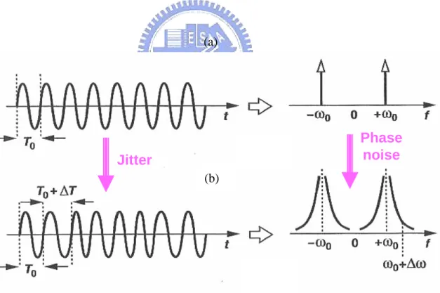
(22) The output SNR of the MRC expressed by Nr. γ=. ∑w. ( l )* ( l ) 2. h. l =1. σ. Nr. 2. ∑w. (2.5) (l ) 2. l =1. can be maximized by applying the Cauchy-Schwartz inequality defined as Nr. Nr. ∑ a(l )*b(l ) ≤ ∑ a(l ) 2. l =1. l =1. 2. Nr. ∑b. (l ) 2. (2.6). l =1. where the equality in (2.6) holds for w( l ) = h ( l ) for all l, which provides the weighting coefficients for MRC. This means that the heavily faded antennas, which are less reliable, are counted less than the less faded antennas, which are more reliable, and vice versa. Substituting w( l ) = h ( l ) into (2.5) leads to the SNR of MRC given by. γ MRC =. 1. σ2. Nr. ∑w. (l ) 2. (2.7). l =1. Noting that | w(l ) |2 / σ 2 is the post-processing SNR for the lth receive antenna, and (2.7) is just the sum of the SNRs for each receive antenna, which means γ MRC can be large even when the individual SNRs are small. It can also be proved that the MRC is the optimal combining technique in the sense of MMSE [25]. In Chapter 4, we will compare various receive diversity schemes in detail.. 2.2. Phase Noise Phenomenon. The time-domain behavior of phase noise effects introduced by the local oscillator in any receiver is called jitter, which is defined as the variation in the time of the significant instants such as zero crossings, as shown in Fig. 2.1. Alternatively, jitter is the deviation of each period from the ideal value as shown in Fig. 2.2. Since phase noise is the Fourier Transform of the jitter introduced by random Gaussian noise, phase noise may be modeled as Wiener process [13]. Phase noise can be interpreted as a parasitic phase modulation in the oscillator’s signal, which ideally would be a unique carrier with constant amplitude and frequency [14]. It has been modeled for simulation purposes as a phase modulation of the subcarrier. The modulated signal is a zero mean white Gaussian random process φW (n) with variance σ W2 . The corresponding 7.

(23) autocorrelation function is given by. RφW (k ) = σ W2 iδ (k ). (2.8). And its power spectral density is given by SφW ( f ) =. ∞. ∑ Rφ. k =−∞. W. (k )ie − j 2π fk = σ W2. (2.9). It has been lowpass filtered with an impulse response hLPF (n) , so that its power spectral density becomes Sφ ( f ) = SφW ( f )i H LPF ( f ). 2. (2.10). where H LPF ( f ) denotes the Fourier Transform of hLPF (n) . In (2.10), Sφ ( f ) is the power spectral density of phase noise and is modeled as Wiener process generated by Gaussian process passing through the lowpass filter as Fig. 2.3. Phase noise variance is also used as a parameter that will be easy to relate to commonly used phase noise specifications.. 2.2.1 Theoretical Analysis of Phase Noise in OFDM Systems For the sake of simplicity, we will not consider the cyclic prefix and assume that the channel is flat. Therefore, the signal only affected by phase noise φ ( n) at the receiver is given by. y (n) = x(n)ie jφ ( n ). (2.11). In order to separate the signal and phase noise terms, let us suppose that φ ( n) is small, so that. e jφ ( n ) ≈ 1 + jφ (n). (2.12). After FFT, the transformed signal is given by Yk = X k +. j N. N −1. N −1. r =0. n=0. ∑ X r ∑ φ (n)e j (2π / N )( r −k ) n = X k + ε k. (2.13). where N is the number of subcarriers, the suffix k denotes the kth tone in one OFDM symbol and error term ε k for each tone resulting from some combination of all of them is added to the useful signal. Let us analyze more deeply this phase noise contribution: 8.

(24) (1). If r = k: common phase error (CPE). εk =. N −1 j X k ∑ φ ( n ) = j i X k iΦ N n =0. (2.14). We have a common error added to every tone that is proportional to its value multiplied by a complex number jΦ , which is a rotation of the constellation given by Φ=. 1 N. N −1. ∑ φ ( n). (2.15). n=0. Since this rotation is identical for all the subcarriers, the phase difference between consecutive symbols can be obtained with the aid of pilots induced in the OFDM frame and corrected. (2). If r ≠ k: ICI. εk =. j N. N −1. N −1. ∑ X ∑ φ ( n)e r =0 r ≠k. r. j (2π / N )( r − k ) n. (2.16). n=0. This term corresponds to the summation of the information of the other N − 1 subcarriers multiplied by some complex number which comes from an average of phase noise with a spectral shift. This result is also a complex number that is added to each subcarrier’s useful signal and has the appearance of Gaussian noise. It is normally known as ICI or loss of orthogonality.. 2.3. Doppler Shift. The relative motion between the base station and the mobile results in random frequency modulation due to different Doppler shifts on each of the multipath components [25]. Doppler shift will be positive or negative depending on whether the mobile receiver is moving toward or away from the base station. Consider a mobile moving at a constant velocity v, along a path segment having length d between points X and Y, while it receives signals from a remote source S, as illustrated in Fig. 2.4. The difference in path length traveled by the wave from source S to the mobile at points X and Y is ∆l = d cos θ = v∆t cos θ , where ∆t is the time required for the mobile to travel from X to Y, and θ is assumed to be the same at points X and Y since the source is assumed to be very far away. The corresponding phase change in the received. 9.

(25) signal can be expressed by 2π∆l. ∆φ =. =. λ. 2π v∆t. λ. cos θ. (2.17). According to (2.17), the apparent change in frequency, or Doppler shift, denoted by f d , is given by fd =. 1 ∆φ v i = icos θ 2π ∆t λ. (2.18). It can be seen from (2.17) that if the mobile is moving toward the direction of arrival of the wave, Doppler shift is positive, and if the mobile is moving away from the direction of arrival of the wave, Doppler shift is negative. Thus, we can understand that Doppler shift increases the signal bandwidth.. 2.3.1 Theoretical Analysis of Doppler Shift in OFDM Systems In mobile radio environment, the channel impulse response model for one data block is expressed as M −1. h(n) = ∑ hl e. j. 2π ε l ( n − nl ) N. (2.19). l =0. where M denotes the total number of propagation paths, and nl and ε l = f dl / ∆f , with ∆f. being the subcarrier separation, are the delay chip number and the. normalized frequency offset associated with the lth path, respectively [26]. For each path, the amplitude of hl is Rayleigh distributed. Since the spectral behavior of OFDM is more important than the temporal behavior of the time domain, the analysis of the frequency domain representation of the channel response is preferred. Consider one typical path and the channel impulse response of the lth path can be expressed by. hl (n) = hl e. j. 2π ε l ( n − nl ) N. (2.20). Therefore, the corresponding frequency domain response at the kth subcarrier can be obtained by FFT as below. H l ,k. 1 = N. N −1. ∑he n =0. l. j. 2π 2π ε l ( n − nl ) − j nk N N. e. 10. 2π 2π − j ε l nl N −1 − j n ( k −ε l ) 1 N = hl e e N ∑ N n=0. (2.21).

(26) Then, the received frequency domain signal Yl , k is given by 2π 2π − j ε l nl N −1 − j n ( k −ε l ) 1 N Yl , k = hl X k e e N ∑ N n=0. π π − j ε l nl N −1 − j n ( k −ε l ) 1 N N = hlδ (k − r )e e ∑ N n=0 2. 2. 2π. (2.22). 2π. n ( k − r −ε l ) − j ε l nl N −1 − j 1 = hl e N ∑ e N N n=0. Note that the second equation holds due to that the transmitted data is set to be. X k = δ (k − r ) for 0 ≤ r < N . Let us analyze more deeply this Doppler shift contribution: (1). If r = k: CPE and frequency offset 2π. − j ε l nl 1 Yl , k = hl e N N CPE. N −1. ∑e. j. 2π nε l N. (2.23). n=0. Frequency offset. (2). If r ≠ k: ICI 2π. 2π. − j ε l nl N −1 − j n ( k − r −ε l ) 1 Yl , k = hl e N ∑ e N N n=0. (2.24). k ≠r. Therefore, Doppler shift results in three effects which are CPE, frequency offset and ICI.. 2.4. Summary. In wireless communication systems, diversity is a powerful technique for the improvement of system performance. Several types of diversity have already been introduced. In addition, the effects of phase noise and Doppler shift are investigated in OFDM systems. Based on the concepts mentioned above, we will propose diversity reception and phase noise compensation schemes for DVB-T systems in Chapter 4.. 11.

(27) Figure 2.1: Illustration of jitter induced by additive noise.. (a). Phase noise. Jitter (b). Figure 2.2: Illustration of relation between jitter and phase noise. (a) Influence of jitter on signal duration. (b) Influence of phase noise on signal bandwidth.. 12.

(28) Figure 2.3: Modeling phase noise in frequency domain.. Figure 2.4: Illustration of Doppler shift.. 13.

(29) Chapter 3 OFDM-Based DVB System DVB system incorporating the OFDM technique can promise robustness against intersymbol interference (ISI) and efficiency in spectrum utilization. Specifically, OFDM with error correcting coding technique used, frequently referred to as COFDM modulation, is a key ingredient of DVB-T system. In this chapter, we will present some possible schemes of the DVB-T system and show how a DVB-T system benefits from the corresponding scheme. Furthermore, the design tradeoff of the DVB-T system is also included.. 3.1. Review of OFDM. OFDM can be regarded as either a modulation or a multiplexing technique. The basic concept of OFDM is to split a high rate data stream into a number of lower rate streams that are transmitted simultaneously over subcarriers [27]-[28]. In order to eliminate the effect of ISI, each OFDM symbol consists of a guard time, which is chosen to be larger than the maximum delay spread such that the current OFDM symbol never hears the interference from the previous one. However, this will cause ICI due to the loss of orthogonality between subcarriers. As a remedy, OFDM symbols are cyclically extended in the guard time to introduce cyclic prefix, as shown in Fig. 3.1. This ensures that the delayed replicas of an OFDM symbol always have an integer number of cycles within the FFT interval. Consequently, cyclic prefix can successively resolve both ISI and ICI caused by multipath as long as the delay spread of channel is smaller than the length of cyclic prefix. In addition, insertion of cyclic prefix makes the 14.

(30) transmitted OFDM symbol periodic, leading to that the linear convolution processing applied to the transmitted OFDM symbols (containing cyclic prefix) and channel impulse response will be translated into a circular convolution one. According to discrete-time linear system theory, the frequency response associated with the output of a circular convolution is equivalent to the product of the frequency responses associated with the OFDM symbol and channel. Definitely, OFDM is a powerful modulation technique for increments in bandwidth efficiency and simplification in removal of distortion due to a multipath channel. Advances in fast Fourier transform (FFT) algorithm enable OFDM to be efficiently implemented in hardware, even for a large number of subcarriers. The key advantages of OFDM transmission are summarized as follows: 1.. OFDM can effectively deal with multipath delay channels with much lower implementation complexity as compared with that of a single carrier system using an equalizer.. 2.. OFDM can achieve robustness against impulse noise because it possesses a long symbol period compared with an equal data-rate single-carrier system.. 3.. OFDM can support dynamic bit loading technique, in which different subcarriers use different modulation modes depending on the channel characteristic or the noise level. Hence, the system performance can be significantly enhanced in this systematic way.. 3.2. Overview of DVB-T Systems. The DVB organization was formed in September 1993. Along these years, several system specifications have been proposed and become standard in the European Telecommunication. Standard. Institute. (ETSI). or. European. Committee. for. Electrotechnical Standardisation. The term “OFDM-based DVB” system is often rewritten by the “DVB-T” system. The DVB-T system for terrestrial broadcasting is probably the most complex DVB delivery system. The key feature of this system is the employment of COFDM, which is a very flexible wide-band multicarrier modulation system using different levels of forward error correction, time and frequency interleaving and two level hierarchical channel coding [23]-[24]. Basically, the 15.

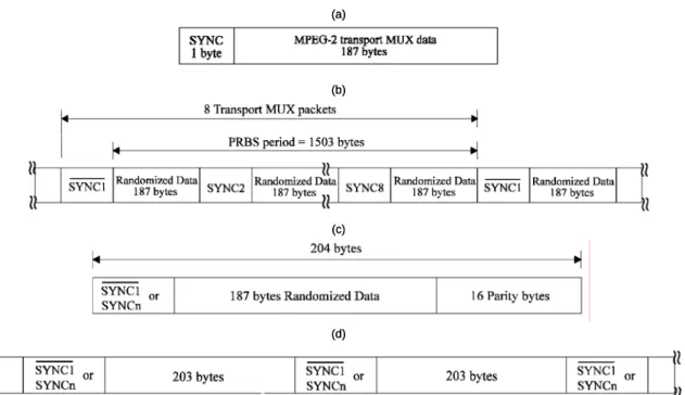
(31) transmitted information is split into a given number (“2k” 1705 or “8k” 6817) of modulated carriers with individual low bit rate, so that the corresponding symbol time becomes larger than the delay spread of the channel. A guard interval (1/4, 1/8, 1/16, 1/32 of the symbol duration) is inserted between successive symbols to avoid ISI and to protect against echoes. Depending on the channel characteristics, different parameters (subcarrier modulation: QPSK, 16QAM, and 64QAM; number of carriers: 2k and 8k; code rate of inner protection, and guard interval length) can be selected leading to different operation modes. Every mode offers a trade-off between net bit rate and protection of the signal (against fading, echoes, etc.). Depending on the selected operation mode, 60 different net bit rates could be obtained ranging from 5 to 32 Mbps. The selection of the COFDM modulation system presents two major advantages that make its use very interesting to terrestrial digital video broadcasting: 1.. COFDM improves the ruggedness of the system in the presence of artificial (long distance transmitters) or natural (multiple propagation) echoes. The echoes may benefit instead of interfering the signal if they fall inside the guard interval.. 2.. COFDM provides a considerable degree of immunity to narrow-band interferers as maybe considered the analogue TV signals; and on the other hand it is seen by those analogue signals as white noise, therefore not interfering or having little effect upon them.. These characteristics enable a more efficient use of the spectrum and the introduction of single frequency networks (SFN). Furthermore, some characteristics of a DVB-T system, as shown in Fig. 3.2, will be discussed as below.. 3.2.1 Scrambler This is a method of removing long runs of 0’s or 1’s in the signal which would otherwise give the receiver a problem at the other end of the channel. This is achieved at the bit level. The pseudo random sequences produced from the incoming bit stream are generated by the polynomial given by 1 + x14 + x15. (3.1). This is realized, as shown Fig. 3.3, with a shift register. Bits 14 and 15 are fed into an XOR gate, then back to the input and also XOR’ed with the data, when enabled, to give 16.

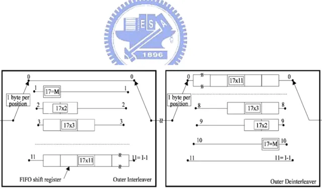
(32) the output. The initialization sequence is loaded every 8 transport packets. Note that this gives a pseudo random binary sequence (PRBS).. 3.2.2 Outer Coder (Reed-Solomon Coder) Reed-Solomon (RS) coding is mathematically very complicated and will not be explained here in any detail. The aim here is simply to give an overview of the coding technique. The coding is a block level code, i.e., it operates over a block of data. The block of data must therefore be constructed prior to the code operation. This puts an overhead on the system in terms of memory and the need for block synchronization. The coding adds 16 additional bytes to the 188 byte transport stream packets, making a final transport stream packet size of 204 bytes. This error correction algorithm, as applied to a transport stream, is characterized by the three numbers n, k and l, where n is the number of bytes in the final transport stream, k is the number of bytes of the original transport stream, and t is the number of bytes that can be corrected. We set the parameters to be n = 204 , k = 188 , and t = 8 . This is referred to as RS (204, 188, 8) shortened code. The RS code effectively specifies a polynomial by generating a large number of points. The RS code can detect and correct up to ( n − k ) / 2 errors. The field generator polynomial is used as. P ( x) = x8 + x 4 + x 3 + x 2 + 1. (3.2). with the code generator polynomial as below. G ( x) = ( x + α 0 )( x + α 1 ). ( x + α 15 ). (3.3). 3.2.3 Outer Interleaver (Convolutional Interleaver) Interleaving is a form of time diversity that is employed to disperse bursts of errors in time. A sequence of data symbols is interleaved before transmission over a bursty channel. If errors occur during transmission, reshaping the original sequence to its original ordering has the effect of spreading the error over time. By spreading the data symbols over time, it is possible to use channel coding, such as RS coding in DVB-T systems, which protects the data symbols from corruption by channel. The interleaver performance depends on the required memory for data storage and the delay in interleaving and deinterleaving, which should be kept as small as possible. In [23], 17.

(33) we obtain that the delay with convolutional interleaver is half the operation time compared with block interleaver and an efficiency of 14.2% for block interleaver and 64% for convolutional interleaver, where efficiency can be defined as the ratio of the length of the smallest burst of errors that can cause the errors correcting capability of the code to be exceeded to the number of memory element used in the interleaver. As stated above, the convolutional interleaver is applied in the outer interleaver of a DVB-T system. The outer coding can correct up to 8 bytes in a transport stream packet. Clearly, if a burst error condition occurs, i.e. a burst of energy from some noise source, then more than 8 bytes within the same packet could become corrupted. The convolution effectively takes these errors and spreads them out over a number of packets, thus allowing the outer coding to be more effective. Fig. 3.4 shows the outer interleaver and deinterleaver. Data is input from the RS outer coding and output to the convolution inner coder. Therefore, there are 12 individual branches with the largest first-input first-output (FIFO) being of length 187 bytes. Input bytes will therefore be delay by 17, 34, 51, …, 187 bytes, depending on the byte index. Fig. 3.5 shows the data format of passing though the scrambler, outer coder and interleaver.. 3.2.4 Inner Coder (Convolutional Coder) Convolutional coding operates at the bit level rather than block level such as RS coding. This has the advantage of the generator not having to store a whole block of data in expensive memory prior to performing the coding. The input stream is fed into shift register stages which have intermediate output taps after each stage. The input stream and various output taps are modulo two added. The DVB-T system actually uses 6 shift register stages and the generator polynomials are shown as. G1 = 171Oct. (3.4). G2 = 133Oct. The architecture as shown in Fig. 3.6 can be considered a state machine. Since there are 6 stages in the DVB-T implementation, this gives rise to 64 states. It is the change from one state to another based on which we can draw the trellis diagram to be applied in the Viterbi decoding algorithm.. 18.

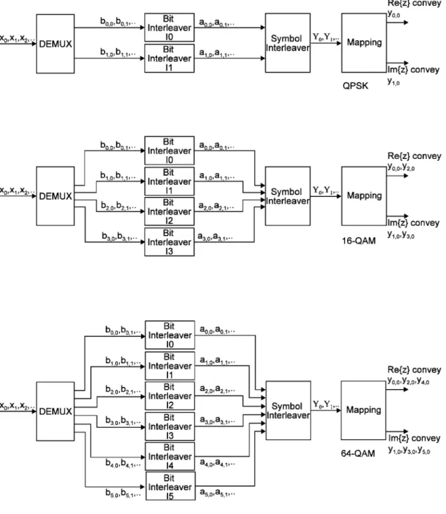
(34) 3.2.5 Inner Interleaver Inner interleaver is also performed to basically spread out the errors and so make the inner coding more effective. The inner interleaving consists of bit-wise interleaving followed by symbol interleaving. Both the bit-wise interleaving and the symbol interleaving processes are block-based.. Bit-Wise Interleaver The input, which consists of up to two bit streams, is demultiplexed into v sub-streams, where v = 2 for QPSK, v = 4 for 16QAM, and v = 6 for 64QAM in Fig. 3.7. The block size is the same for each interleaver, but the interleaving sequence is different in each case. The bit interleaving block size is 126 bits. The block interleaving process is therefore repeated exactly twelve times per OFDM symbol of useful data in the 2k mode and forty-eight times per symbol in the 8k mode. For each bit interleaver, the input bit vector is defined by B (e) = (be ,0 , be ,1 , be ,2 , ..., be ,125 ). (3.5). where be, w denotes the bit number w of inner bit interleaver e, B (e) denotes the input vector to inner bit interleaver e, and e ranges from 0 to v-1. The interleaved output A(e) = (ae ,0 , ae ,1 , ae ,2 , ..., ae ,125 ) is defined by ae , w = be , He ( w) , w = 0, 1, 2,..., 125. (3.6). where ae , w denotes the bit number w of inner bit interleaver output stream e, and. H e ( w) is a permutation function which is different for each interleaver. The H e ( w) is defined as follows for each interleaver I0: H 0 ( w) = w I1: H1 ( w) = ( w + 63) mod 126 I2: H 2 ( w) = ( w + 105) mod 126 I3: H 3 ( w) = ( w + 42) mod 126. (3.7). I4: H 4 ( w) = ( w + 21) mod 126 I5: H 5 ( w) = ( w + 84) mod 126 The outputs of the v bit interleavers are grouped to form the digital data symbols, such that each symbol of v bits will consist of exactly one bit from each of the v interleavers. 19.

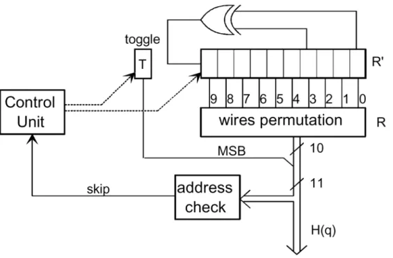
(35) Hence, the output from the bit-wise interleaver is a v bit word y', i.e. y 'w = ( a0, w , a1, w ,..., av -1, w ). (3.8). Symbol Interleaver The purpose of the symbol interleaver is to map the 2, 4 or 6 bit words onto one of the OFDM carriers (1512 for 2k mode or 6048 for 8k mode). The interleaved vector Y = ( y0 , y1 , y2 , ... y N max −1 ) is defined by. yH ( q ) = y 'q for even symbols for q =0,..., N max − 1 yq = y 'H ( q ) for odd symbols for q =0,..., N max − 1. (3.9). where N max = 1512 in the 2k mode and N max = 6048 in the 8k mode. H ( q ) is a permutation function defined by the following. An ( N r − 1) bit binary word R 'i is defined, with N r = log 2 M max , where M max = 2048 in the 2k mode and M max = 8192 in the 8k mode, where R 'i takes the following values:. i = 0,1: R 'i [ N r − 2, N r −3, ..., 1, 0] = 0, 0,..., 0, 0 i = 2 : R 'i [ N r − 2, N r − 3, ..., 1, 0] = 0, 0,..., 0, 1 2 < i < M max : { R 'i [ N r − 3, N r − 4,..., 1, 0] = R 'i −1[ N r − 2, N r − 3,..., 2, 1];. (3.10). 2K mode : R 'i [9] = R 'i −1[0] ⊕ R 'i −1[3] 8K mode : R 'i [11] = R 'i −1[0] ⊕ R 'i −1[1] ⊕ R 'i −1[4] ⊕ R 'i −1 [6] } A vector Ri is derived from the vector R 'i by the bit permutations given in Table 3.1. The permutation function H ( q ) is defined by the following algorithm. q = 0; for (i = 0; i < M max ; i = i + 1) { H (q ) = (i mod 2) × 2 N r −1 +. Nr −2. ∑ R ( j) ⋅ 2 ; j. j =0. (3.11). i. if ( H (q ) < N max ), q = q + 1; } A schematic block diagram of the algorithm used to generate the permutation function is represented in Fig. 3.8 for the 2k mode. 20.

(36) 3.2.6 Subcarrier Modulation Mapping and OFDM Frame Structure The system uses OFDM transmission. All data carriers in one OFDM frame are modulated using either QPSK, 16QAM, 64QAM, non-uniform 16QAM or non-uniform 64QAM constellations. The exact values of the constellation points are given by. d = K MOD × (n + jm). (3.12). where K MOD is the normalization factor and z ∈ {n + jm} with values of n, m is given by Table 3.2. The basic structure of what is known as an OFDM signal is a variable number of frequency carriers, either 1705 (known as 2k mode) or 6817 (known as 8k mode) as Table 3.3. These carriers are spaced in such a way as to allow them to fit into the 7.61 MHz bandwidth. These carriers can be shown in Fig. 3.9 and described as follows. 1.. Data: with a variable number of bits per carrier. 2.. Transmission parameter signalling (TPS): transmission information. 3.. Pilot: for receive synchronization, there are two types both transmitted at boosted power levels a.. Continual: there are 177 tones in 8k mode, and 45 tones in 2k mode. These always are at the same frequency in different OFDM symbols. These pilots are used to compute the CPE. The CPE is an error that is introduced into the signal due to the local oscillator’s phase noise. The CPE is a change in phase of all carriers within an OFDM symbol compared to the next OFDM symbol.. b.. Scattered: there are 524 tones in 8k mode, and 131 tones in 2k mode. Specified insertion pattern within the symbol. These pilots are used to estimate the channel distortion.. On the other hand, the guard interval is a replication of the end of the symbol and is added to the beginning of the symbol. The guard interval length of DVB-T system can be 1/4, 1/8, 1/16 or 1/64 of the symbol duration. There are two main reasons for the insertion of a guard interval. The first one is to combat against the ISI. The other is to allow the receiver to identify the start of a symbol. Finally, Table 3.4 gives simulated BER performance anticipating “perfect channel estimation and no phase noise” for various combinations of channel coding and modulations. 21.

(37) 3.3. Synchronization in DVB-T Systems. One of the major drawbacks of an OFDM system is its high sensitivity to synchronization errors, in particular, to carrier frequency errors. In an OFDM system, the pilot or cyclic prefix is used for the sake of synchronizing OFDM signals. An algorithm with the pilot used, referred to as the pilot-based synchronization, is developed based on a two-stage procedure. First, the transmitter encodes a number of reserved subchannels with the given phases and amplitudes. A correlation detector is then performed on the received signal to extract the synchronization information at the pilot tones. On the other hand, a scheme with the cyclic prefix used, referred to as the cyclic-prefix-based synchronization, can enable the self-synchronization [28]. The block diagram of synchronization techniques in DVB-T systems is illustrated in Fig. 3.10. The corresponding function of each block is investigated as below.. 3.3.1 Coarse Estimation. Timing. and. Frequency. Offset. Fig. 3.11 shows a cyclic-prefix-based synchronizer for coarse timing and frequency offset estimation [29]. The cyclic prefix generated by duplicating the last N cp samples of the N c -sample OFDM symbol is prefixed in the ( N c + N cp ) -sample. OFDM symbol. Note that the duration of the cyclic prefix should be greater than the maximum delay of the channel impulse response to eliminate ISI. Since the receiver cannot obtain the symbol starting position within the observation interval preliminarily, a likelihood function based on the consecutive samples of the received OFDM signal y along with moving average at time instant i is suggested for coarse timing. synchronization and is given by. ⎧ N cp −1 ⎫ ˆj = a rg max ⎪⎨ ∑ y * ( j + i − N c ) y ( j + i ) ⎪⎬ j ⎩⎪ i =0 ⎭⎪. (3.13). where ˆj and y (i ) denote the estimated symbol starting position and the ith sample of the received OFDM signal. In addition, frequency offset estimation is given by f coarse =. ⎧⎪ Ncp −1 ⎫⎪ 1 arg ⎨ ∑ y* ( j + i − N c ) y ( ˆj + i ) ⎬ 2π N cTsample ⎩⎪ i = 0 ⎭⎪ 22. (3.14).

(38) where Tsample denotes the sample duration. Since coarse timing and frequency offset estimates in (3.13) and (3.14), respectively, are usually distorted due to noise effect, we can average the estimates over several successive OFDM symbols to enhance the accuracy in timing and frequency offset estimation.. 3.3.2 Fine Timing Estimation Performance of coarse timing estimation will degrade due to the channel random noise, which will induce the estimation error of one or two samples. Therefore, a fine timing estimator is necessary for enhancing its robustness against noise. Specifically, as the starting position estimate ˆj is obtained, we correlate totally 7 OFDM symbols before and after ˆj with known continual pilots of the DVB-T system. The exact symbol starting position can be determined by maximizing the correlator output. Mathematically speaking, the algorithm, referred to as an early-late fine timing estimation, is given by. ⎧⎪ N p ,cont * j = max ⎨ ∑ Yk ( ˆj + j ) ⋅ X k ,cont j ⎩⎪ k =1. ⎫⎪ ⎬ , j = −3, −2, ⎭⎪. , 2,3. (3.15). where j is the estimated fine time index, N p ,cont is the number of the continual pilots, and X k ,cont is the value of the kth continual pilot, with k being the frequency index.. 3.3.3 Fine Frequency Estimation In order to further improve the performance in frequency offset estimation, a fine frequency offset estimator, as shown in Fig. 3.12, is constructed based on the continual pilots X k ,cont and given by f fine =. ⎧⎪ N p ,cont 1 ⎪ *⎫ arg ⎨ ∑ X k + Nc ,cont X k ,cont ⎬ 2π ( N c + N cp )Tsample ⎪⎩ k =1 ⎭⎪. (3.16). Similarly, several OFDM symbols can be used to enhance the accuracy in timing and frequency offset estimation [30].. 23.

(39) 3.3.4 Frame Timing Estimation Generally, the receiver performs the timing estimation at the beginning of the reception [31]. However, clock offset may cause sample drifting during one frame duration. Therefore, frame timing synchronization is necessary for every frame. Substantially, the second to 17 bits of the TPS pilot can be used to estimate frame starting position and the corresponding likelihood function for frame timing synchronization is given by. ⎧⎪ N p ,TPS * j = max ⎨ ∑ Yk ( j ) ⋅ X k ,TPS j ⎩⎪ k =1. ⎪⎫ ⎬ ⎭⎪. (3.17). where N p ,TPS denotes the number of bits associated with the TPS pilot for frame synchronization, and X k ,TPS denotes the TPS pilot. The frame timing estimation in (3.17) possesses two advantages: one is that the TPS pilot is more reliable due to the extra protection of the Bose-Chaudhuri-Hocquenghem (BCH) coding. The other is that we only need 16 synchronization bits in one frame, leading to a reduction of computational complexity.. 3.4. Channel Estimation in DVB-T Systems. In wideband mobile communication systems, under the assumption of a slow fading channel, in which the channel transfer function is stationary within several OFDM data symbols, preambles or training sequences can be used to estimate the channel response for the following OFDM data symbols. However, in practice, the channel response may significantly vary even within one OFDM data block. Therefore, in DVB-T systems, it is preferable to estimate the channel characteristic based on the pilot signals in each individual OFDM data block. The conventional channel estimation involves a two-stage procedure. First, the channel responses associated with the pilot tones are estimated. Second, interpolation technique is used to obtain channel responses of the data tones. We will introduce two pilot-aided channel estimation methods. One is least square (LS) channel estimation, together with piecewise-linear interpolation. The other is application of low-pass filtering on the transformed pilot tones to reduce the Gaussian noise and ICI effects.. 24.

(40) 3.4.1 Least Square Channel Estimation with Linear Interpolation Consider an OFDM system with N p , scat scattered pilot signals. The received pilot signal in vector form can be given by Yscat = X scat H scat + N scat. ⎡ X scat (0) ⎢ =⎢ ⎢ 0 ⎣. 0. X scat ( N p , scat. ⎤⎡ ⎤ H scat (0) ⎥⎢ ⎥ (3.18) ⎥⎢ ⎥ + N scat − 1) ⎥⎦ ⎢⎣ H scat ( N p , scat − 1) ⎥⎦. X scat. H scat. where X scat , H scat , and N scat denote the scattered pilot signals, the corresponding channel responses, and the noise, respectively [32]. According to the LS criterion, the channel transfer function can be obtained by. a rg min Yscat − X scat H scat. 2. (3.19). H scat. whose solution is given by 1 H scat , LS = X −scat Yscat. (3.20). From (3.20), the channel estimate can be obtained by dividing the received signals by the known scattered pilots. This implies that the LS channel estimator is easier to implement. As the estimation of the channel transfer functions of pilot tones is determined, the channel responses of data tones are then constructed by the linear interpolation technique. Note that we consider a linear interpolation method due to simplicity. With the linear interpolation used, two successive pilot subcarriers are used to compute the channel responses of data subcarriers located between these two pilot tones. Mathematically speaking, the estimated channel response of data subcarrier l within the m th and ( m + 1) th pilot tones is given by l l H (mL + l ) = (1 − ) H scat (m) + H scat (m + 1) L L l = H scat (m) + H scat (m + 1) − H scat (m) , 0 < l < L L. (. ). (3.21). where L = N M , with N and M being the number of total subcarriers and the number of pilot signals. Its schematic diagram of the pilot-based channel estimation with linear interpolation is shown in Fig. 3.13. It is noteworthy that this method needs lower computational complexity than those of channel estimation methods. 25.

(41) 3.4.2 Lowpass Filtering in Transform Domain LS-based channel estimation can achieve a better performance in a slow fading channel as long as the noise power is moderately small. However, this assumption is impractical due to the fact that a wideband radio channel is usually time-variant, frequency selective, and noisy. The pilot signals may be corrupted by ICI introduced by the fast variation of the mobile channel. In addition, the performance in channel estimation will significantly degrade because of noise. As a remedy, a novel channel estimation incorporating lowpass filtering in the transform domain, as shown in Fig. 3.14, is utilized to alleviate the effects of both ICI and noise [33]. The design involves the following procedure. 1.. Rough channel response obtained by LS channel estimation We first perform initial estimation of the channel responses at pilot locations with. a simple LS method used. That is, Y (k ) N (k ) Hˆ scat ,ls (k ) = scat = H sact (k ) + scat , k = 0, …, N p , scat -1 X scat ( k ) X scat ( k ). (3.22). where X scat and N scat = N scat ,noise + N scat , ICI denote the pilot signal and the noise component consisting of ICI and noise, respectively. 2.. Noise and ICI reduction Since the true channel response H scat ,ls in (3.22) is slowly varying with respect to. the noise component N scat , the “virtual high frequency” and “virtual low frequency” regions in the transformation of the estimated channel response will be mainly contributed by the true channel response and the noise, respectively. Note that the quotation marks denote the transform domain. An example is shown in Fig. 3.15. This suggests that these two components can be successfully separated by transforming the estimated channel responses of the pilot tones into the transform domain with discrete Fourier transform (DFT) or FFT. The transformation of Hˆ scat ,ls (k ) is given by i. G scat ( w) =. N scat −1. ∑ k =0. ⎛ ⎞ 2π Hˆ scat ,ls (k ) exp ⎜ − j kw ⎟ ⎝ N scat ⎠. (3.23). where w is the transform domain index for w ∈ [0, N p , scat − 1] . An ideal lowpass filter is then performed on the transformed data, leading to. 26.

(42) ⎧⎪ i G ( w), 0 ≤ w ≤ wc , N p , scat - wc ≤ w ≤ N p , scat -1 G scat ( w) = ⎨ scat ⎪⎩0, otherwise. (3.24). where wc is the “virtual cutoff frequency” of the filter. After filtering, noise and ICI effects can be effectively reduced. 3.. Interpolation approach Under the assumption of slow-variation, the channel transfer function can be. viewed as the sum of several sinusoidal functions with respect to k. However, the number and the “virtual frequencies” of the sinusoids vary due to the changing in the mobile radio channel. To avoid the model mismatch problem, we do not transform. G scat ( w) back to frequency domain and then perform interpolation. Instead, a high-resolution interpolation approach based on zero-padding is used. First, the N p , scat -sample transform-domain sequence G scat ( w) is extended to an N c -sample. sequence G (q) by padding with N c − N p , scat zero samples at the “virtual high frequency” region as follows: ⎧G scat (q ), 0 ≤ q ≤ wc ⎪⎪ G (q ) = ⎨0, wc < q < N c − wc ⎪ ⎪⎩G scat (q − N c + N p , scat ), N c − wc ≤ q ≤ N c − 1. (3.25). This N c -sample sequence G (q) , in its physical meaning, is the Fourier transform of the desired estimate of the channel transfer function. By performing an N c -point inverse DFT/FFT (IDFT/IFFT), the estimated transfer function is obtained as Nc −1 ⎛ 2π ⎞ H filter (k ) = a ∑ G (q ) exp ⎜ j qk ⎟, 0 ≤ k ≤ N c -1 q =0 ⎝ Nc ⎠. (3.26). where a denotes normalized coefficient term after IDFT. 4.. Dynamic selection of cutoff frequency According to (3.24), the accuracy of the channel estimation with lowpass filtering. is substantially dependent on the “virtual cutoff frequency” wc . With a large value of. wc selected, noise and ICI effects can only be reduced slightly, while the desired signal will be suppressed with a small value of wc used. A proper value of wc can be determined adaptively by the ratio.. 27.

(43) N scat −1 ⎡ wc 2 2⎤ + G ( w ) Gscat ( w) ⎥ ⎢ ∑ scat ∑ w= 0 w = N scat − wc ⎦ R= ⎣ N scat −1 2 ∑ Gscat (w). (3.27). w= 0. i. where Gscat ( w) is the average of G scat ( w) of the present OFDM symbol and those of ten previous OFDM symbols. By a rule of thumb, the ratio R is selected within 0.9 and 0.95. The channel estimator with lowpass filtering can achieve better performance in the penalty of higher computational complexity. This is because additional operations are necessary for the implementation of a lowpass filter, DFT/FFT, and IDFT/IFFT.. 3.5. Computer Simulations. Computer. simulations. are. conducted. to. evaluate. the. performance. of. synchronization and channel estimation in a DVB-T system. The channel model employed is given by K −1. ρ 0 x(t ) + ∑ ρi e − jθ x(t − τ i ) i. y (t ) =. i =1. (3.28). K −1. ∑ρ i =0. 2 i. where x(t ) and y (t ) are input and output signals, K is the number of fingers set to be 20, and θi , ρi and τ i denote the phase shift from scattering, the attenuation, and the relative delay associated with ith path, respectively. Note that the first term in the numerator in (3.26) represents the line of sight ray. The parameter setting of channel response is summarized in Table 3.5. In simulation, the relationship between SNR and. Eb N 0 can be defined as Eb Ts. Es Eb T ⋅M bit power 1 = = = s = SNR ⋅ N 0 noise power N ⋅ 1 N0 ⋅ B M 0 Ts. (3.29). When the system transmit power is normalized to one, then the noise power is given by. σ 2 corresponding to a specific Eb N 0 can be generated by N σ2 = 0 Eb. (3.30). where Es is the symbol energy, Ts is the symbol duration, B is the system bandwidth, 28.

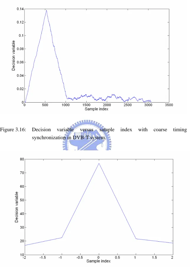
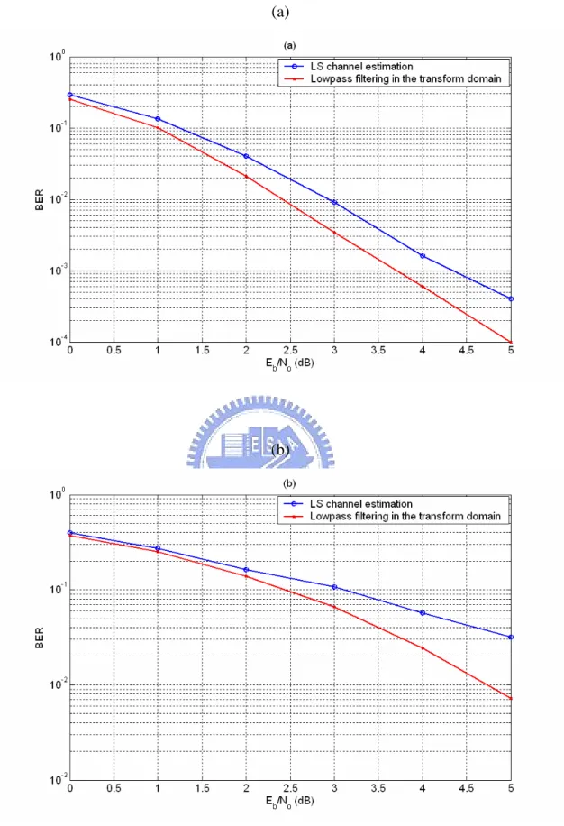
(44) and M is the modulation order. In the first simulation, the performance of synchronization is investigated in a DVB-T system. The simulation parameter setting is listed in Table 3.6. The result of cyclic-prefix-based coarse timing synchronization shown in Fig. 3.16 indicates that coarse timing synchronization may cause an error of one or two samples. Hence, a fine timing synchronization is required to enhance the performance. The result obtained by the pilot-based fine timing synchronization as shown in Fig. 3.17, demonstrates that a precise symbol timing position can be obtained. In the second simulation, the performance of channel estimation is examined in a DVB-T system. The BER versus Eb N 0 plots obtained by the LS channel estimation with linear interpolation and lowpass filtering in the transform domain are shown in Fig. 3.18 (a)-(b) for the mobile speed v of 0 and 20 m/s, respectively. Note that the Jake’s model is used to model the fading channel. From Fig. 3.18 (a), we observe that lowpass filtering can successfully suppress the noise and provides about 1dB improvement as compared with the LS channel estimation for the BER of 6 × 10−4 . This is because that the effect of ICI is negligible for low velocity. On the contrary, in the case of high velocity, the performance of both methods is degraded due to ICI, but the lowpass filtering slightly outperforms than the LS method. These simulation results confirm that the lowpass filtering can obtain better performance than the LS channel estimation.. 3.6. Summary. A standard DVB-T system is introduced. The cyclic-prefix based and pilot-based schemes are then constructed to enhance the accuracy of timing and frequency offset estimation over a fading channel. In addition, LS channel estimation with linear interpolation and lowpass filtering in the transform domain are also included for correct estimation of the channel response. A DVB-T system incorporating the previously mentioned technique proves to be robust in a typical urban environment.. 29.

(45) .......... 2. x0. d Nc − 2. x1. 2. IDFT. xNc − Ncp. OFDM signal. D/A. .......... Serial to parallel converter d − Nc +1. Parallel to serial converter. .......... ................. Input data Input data symbols Symbols. d Nc −1. 2. d − Nc. xNc −1. 2. Figure 3.1: Digital implementation of appending cyclic prefix into OFDM signal in transmitter.. Source data. Scrambler Scrambler. Outer Outer coding coding & & interleaving interleaving. Inner Inner coding coding & & interleaving interleaving. Modulation Modulation. Pilot Pilot insertion insertion and and frame frame adaptation adaptation. IFFT IFFT. Guard Guard interval interval insertion insertion. Up Up conversion conversion. Tx. Fine Fine frequency frequency estimation estimation. Impulse Impulse noise noise detection detection. + Channel Channel estimation estimation. Down Down conversion conversion. Impulse Impulse response response shortening shortening. Coarse Coarse timing timing estimation estimation. Coarse Coarse frequency frequency estimation estimation. FFT FFT. Fine Fine timing timing estimation estimation. Frame Frame timing timing estimation estimation Phase Phase noise noise & & I/Q I/Q imbalance imbalance compen. compen.. Figure 3.2: Transceiver architecture for DVB-T system. 30. Diversity Diversity combining combining or or selection selection. Data Data detection detection. Rx.

(46) Figure 3.3: Scrambler/descrambler schematic diagram in DVB-T system.. Figure 3.4: Conceptual diagram of outer interleaver and deinterleaver DVB-T system.. 31.

(47) (a). (b). (c). (d). Figure 3.5: Data format of DVB-T system. (a) MPEG-2 transport MUX packet. (b) Randomized transport packets: Sync bytes and randomized data bytes. (c) RS(204, 188, 8) error protected packets. (d) Data structure after outer interleaving.. Figure 3.6: Mother convolutional code of rate 1/2 in DVB-T system.. 32.

(48) Figure 3.7: Mapping of input bits onto output modulation non-hierarchical transmission modes in DVB-T system.. 33. symbols,. for.

(49) Figure 3.8: Block diagram of symbol interleaver address generation scheme for 2k mode in DVB-T system.. Figure 3.9: Frame structure in DVB-T system.. 34.

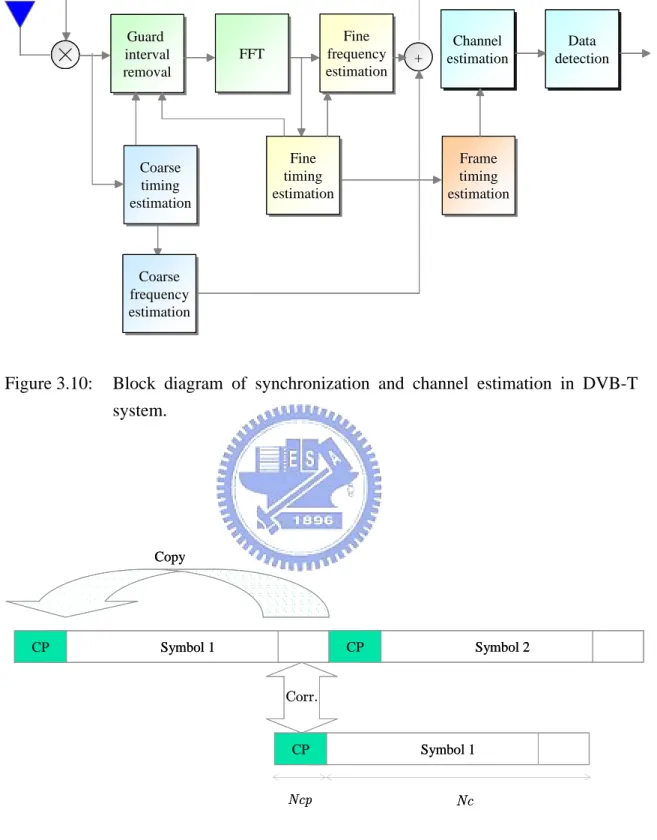
(50) Guard Guard interval interval removal removal. Coarse Coarse timing timing estimation estimation. Fine Fine frequency frequency estimation estimation. FFT FFT. Fine Fine timing timing estimation estimation. +. Channel Channel estimation estimation. Data Data detection detection. Frame Frame timing timing estimation estimation. Coarse Coarse frequency frequency estimation estimation. Figure 3.10:. Block diagram of synchronization and channel estimation in DVB-T system.. Copy. CP. CP. Symbol 1. Symbol 2. Corr.. Figure 3.11:. CP. Symbol 1. Ncp. Nc. Illustration of OFDM signal with cyclic prefix for coarse timing and frequency offset synchronization.. 35.

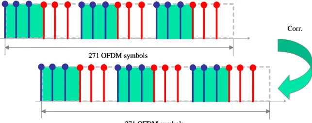
(51) Corr.. 271 OFDM symbols. 271 OFDM symbols. Figure 3.12:. Illustration of pilot-based correlation for fine frequency synchronization in synchronization and channel estimation in DVB-T system.. f. Channel response at the pilot tone. Figure 3.13:. Illustration of pilot-based channel estimation with linear interpolation in DVB-T system.. 36.

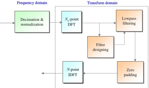
(52) Frequency domain. Decimation Decimation & & normalization normalization. Transform domain. N Npp-point -point DFT DFT. Lowpass Lowpass filtering filtering. Filter Filter designing designing. N-point N-point IDFT IDFT. Figure 3.14:. Zero Zero padding padding. Block diagram of channel estimation with lowpass filtering in transform domain in OFDM system.. High “virtual frequency” component. Figure 3.15:. Estimated channel amplitude responses in transform domain of OFDM system.. 37.

(53) Figure 3.16:. Decision variable versus sample synchronization in DVB-T system.. Figure 3.17:. Decision variable versus sample index with fine timing synchronization in DVB-T system.. 38. index. with. coarse. timing.

(54) (a). (b). Figure 3.18:. BER performances versus Eb N 0 of channel estimation methods in DVB-T system with mobile speed v of (a) 0 m/s. (b) 20 m/s.. 39.