Message Ferry Routing Algorithm for Data Collection
in Partitioned and Buffer-Limited Wireless Sensor Networks
JYH-HUEI CHANGAND RONG-HONG JAN
Department of Computer Science National Chiao Tung University
Hsinchu, 300 Taiwan
In some particular environments such as battlefield, disaster recovery and wide area surveillance, most existing routing algorithms will fail to deliver messages to their des-tinations. Thus, it is an important research issue of how to deliver data in disconnected wireless sensor networks. This paper presents two efficient message ferry routing algo-rithms, denoted as MFRA1 and MFRA2, for data collection in disconnected wireless sensor networks. Both algorithms are designed to find feasible routes for the message ferry such that the buffers of sensors will not overflow after a complete sequence. A complete sequence is the visit sequence of message ferry which visits every sensor node at least once. We find the shortest sequence for message ferry which visits every sensor exactly once and then we check the feasibility of the visit sequence. If there is a sensor overflow, MFRA1 and MFRA2 fix the overflow by partitioning the initial visit sequence into some sub-sequences such that the ferry visits the overflow node twice in the result-ing sequence. The above process will continue until a feasible solution is found. Simula-tion results show that both MFRA1 and MFRA2 are better than other schemes in terms of the amount of data lost, because the other schemes neglect the case of sensor over-flow.
Keywords: message ferry, routing algorithm, data collection, sensor networks, partitioned networks
1. INTRODUCTION
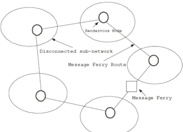
In disconnected wireless sensor networks, most existing routing algorithms will fail to deliver messages to their destinations. The Message Ferry scheme is an approach for message delivery in the disconnected wireless sensor network. As shown in Fig. 1, there is a wireless sensor network with several separated sub-networks. Each sub-network has a rendezvous node to connect and buffer the data. A special node, called Message Ferry, visits these rendezvous nodes to collect the buffered data of the sensing field based on a pre-defined route. The message ferry route problem is to find a route for message ferry to visit rendezvous nodes and collect data.
1.1 Our Proposed Scheme
The previous schemes focus on the routing problems under the assumption that the buffer size of each sensor node is unlimited. These schemes do not deal with the condi-tion that the sensor may overflow and thus the sensing data will lose.
In real applications, there are different kinds of sensors such as surveillance sensors and data sensors. The surveillance sensor has high sampling rate to capture video mes-
Fig. 1. Example of message ferry scheme.
sages. The data sensor has low sampling rate to collect temperature or noise data. In such a sensing environment, each sensor has a limited buffer size and thus the surveillance sensor may overflow before the message ferry visits all sensor nodes. It is a serious prob-lem that a sensor loses critical messages due to overload. Therefore, how to avoid over-flow should be an important research issue in the message ferry routing problem. This paper presents two novel message ferry routing algorithms to find feasible solutions un-der the limited buffer size constraint for disconnected wireless sensor networks.
In our network model, we assume that the message ferry has infinite memory and can move to visit each rendezvous node. All sensors are static and have a limit buffer size. The main idea of the proposed Message Ferry Routing Algorithms (MFRA1 and MFRA2) is that we find the shortest visit sequence for message ferry which visits every sensor exactly once and then we check the feasibility of the visit sequence. If there is a sensor overflow, MFRA1 and MFRA2 fix the overflow by partitioning the initial visit sequence into some sub-sequences such that the ferry visits the overflow node twice in the resulting sequence. Then, we check the feasibility of the current sequence until a fea-sible solution is found.
Simulation results show that both MFRA1 and MFRA2 algorithms perform better than Greedy and Nearest Neighbor algorithms in term of the amount of data lost. Greedy and Nearest Neighbor algorithms will lose data when sensors overflow. MFRA1 and MFRA2 algorithms can solve the problem of buffer overflow.
The remainder of this paper is organized as follows. In section 2, we define the problem formulation and network model. Section 3 illustrates the details of the proposed algorithms. The simulation results and performance analysis are shown in section 4. Fi-nally, the conclusions are given in section 5.
1.2 Related Work
Several schemes have been proposed to solve the message ferry route problem in partitioned wireless ad hoc networks [1-5]. In [1], the authors propose a message ferry scheme to solve the data delivery problem in high-partitioned wireless ad hoc networks.
In [2], the authors introduce a non-randomness in the movement of nodes to improve data delivery performance and reduce the energy consumption in sensor nodes. Epidemic routing [4] is also a well-known routing method for partitioned wireless ad hoc networks. In this scheme nodes forward messages to other nodes they meet. However, this scheme transmits many redundant messages. Compared to Epidemic routing, message ferry scheme is very efficiency in data delivery and energy consumption. However, the syn-chronization between nodes and ferry is a problem in the message ferry scheme. An op-timized way-points (OPWP) algorithm [3] was proposed. It generates a ferry route to achieve good performance without any online collaboration between nodes and the ferry. OPWP outperforms other naive ferry routing schemes.
Many studies deal with efficient routing for intermittently connected mobile ad hoc networks [6-13]. In [6, 7], the authors proposed a routing scheme with two types of fer-ries and gateways. This scheme improves delivery rate and delay without online collabo-ration between ferry and mobile nodes. However, the local message ferry, global mes-sage ferry and gateway nodes of this scheme need more resources to buffer the mesmes-sages. In [8], the authors proposed single-copy routing schemes that use only one copy per mes-sage, and hence significantly reduce the resource requirements of flooding-based algo-rithms. In [9], the authors proposed a routing scheme that sprays a few message copies into the network, and then routes each copy independently toward the destination. This scheme can reduce the delay in flooding-based scheme.
Some studies deal with the data scheduling problem for message ferry [14, 15]. In [14], the authors present an elliptical zone fording (EZF) scheme for a ferry to deliver messages among partition nodes that are moving around. EZF scheme gives priority to urgent messages that are already in the message ferry buffer. However, there may be ur-gent message waiting to be picked up at other nodes that have closer deadlines than the most urgent message in the delivery up queue. Three ferry routes with look-ahead schemes were proposed in [15] to overcome the drawback of EZF scheme. The dynamic look-ahead scheme provides the best performance compared with other schemes.
Several studies focus on mobile element scheduling problem [16-18] for wireless sensor networks (WSNs). The mobile element works as a mobile sink in WSNs, which is similar to the message ferry. In [16], the authors present an architecture to connect sen-sors in sparse sensor networks. The advantage of this scheme is the potential of large power savings that can occur at the sensors because communication takes place over a short-range. Its disadvantage is the increasing latency because sensors have to wait for a mobile element to approach before the transfer can occur. In [17], the authors proposed a load balancing algorithm to balance the number of sensor nodes that each mobile element services. The network scalability and traffic may make a single mobile element insuffi-cient. Using multiple mobile elements scheme can overcome this problem.
2. PROBLEM FORMULATION AND NETWORK MODEL
2.1 Network Model
(1) A set of sensors are randomly deployed in a two-dimensional sensing area. These sensors form a disconnected network. The buffer size of each sensor is constant. (2) Each sub-network has a sensor node, called rendezvous node, which collects and
buffers the sensing data from other nodes. Each sensor node has different sampling rate to sense data and has to deliver sensing data to the rendezvous node in its sub- network.
(3) A message ferry visits each rendezvous node to collect data. The moving speed of the message ferry is constant. The message ferry works as a mobile sink and has infinite memory. When the message ferry visits a rendezvous node, the buffer of the rendez-vous node will refresh to empty. Message ferry and sensor nodes have the same transmission range.
(4) The data transmitting time from a rendezvous node to the message ferry is ignored. (5) Without loss of generality, we assume that there is only one sensor node in each sub-
network. Thus, the terms, rendezvous node and sensor node, are used interchangeably in the following sections.
2.2 Problem Formulation
We formulate the problem as follows. Let N = {n1, n2, …, nm} be a set of m sensors in a two-dimensional sensing field, and let dij be the distance between nodes ni and nj. The message ferry visits each sensor node at a constant speed to collect sensing data. We want to find a visit sequence for the message ferry such that the buffer of each sensor does not overflow between two visits. A complete sequence is defined as the visit se-quence of message ferry which visits every sensor node at least once and returns to the start sensor node. That is, a sequence ni1, ni2, …, nik, k ≥ m, is said to be a complete
se-quence if ni1 = nik and ∪
k
j=1{nij} = N. The message ferry can repeat this complete sequence
again and again if the sequence is feasible. Thus, any sensor node nij in the sequence ni1, ni2, …, nik-1, ni1 can act as start node and the resulting sequence nij, nij+1, …, nik-1, ni1, ni2, …, nij is equivalent to the sequence ni1, ni2, …, nik-1, ni1. Next, we define the travel time ti1 of
message ferry between two visits for node ni1 with respect to the complete sequence ni1, ni2, …, nik-1, ni1 as follows. 1. If nij ≠ ni1, j = 2, …, k − 1, then 1 1 1 1 2 1 ( kj i ij j ) i ik i d d t s + − − = + =
∑
where s is the speed of message ferry.2. If ni1 in the complete sequence ni1, ni2, …, nik-1, ni1, repeats p + 2, (p ≥ 1) times, say nih1
= ... = nihp = , then 2 1 1 1 1 1 1 1 1 2 1 1 1 ( ) max j j , j j , , p j j k . k h h i i i i i i i i j h j h j i d d d d t s s s + − + + − − − = = = ⎧ + ⎫ ⎪ ⎪ ⎨ ⎬ = ⎪ ⎪ ⎩ ⎭
∑
∑
∑
…In this case, we say the complete sequence ni1, ni2, …, nik-1, ni1 is partitioned into p sub-sequences on the node ni1.
set of sensor nodes N = {n1, n2, …, nm} and the distance between every pair of m sensors
in form of an m × m matrix [dij], where dij > 0. Each sensor node ni has a sensing rate ri to
collect data and a buffer with size bi to store sensing data. The message ferry visits each
sensor node with constant speed s to pick up the sensing data. A complete sequence ni1,
ni2, …, nik, k ≥ m, is a closed path that visits every sensor at least once. The message ferry
routing problem is to find a complete sequence such that the buffer of each sensor does not overflow between two visits. That is, tij ≤ bij/rij for every node nij where tij is the travel
time of message ferry between two visits for node nij with respect to sequence ni1, ni2, …,
nik.
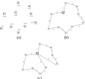
Consider an example of a sensor network with a set of sensor nodes N = {n1, n2, …,
n10}, as shown in Fig. 2 (a), and the distance between every pair of 10 sensors.
Fig. 2. (a) Ten sensors in the sensing field; (b) A least cost visit sequence with one critical node (Node n1); (c) A feasible complete sequence n1, n2, n3, n4, n5, n1, n6, n7, n8, n9, n10, n1.
1 2.3 2.5 4 3 3.8 3.2 3.5 1 1 2 2.7 4.5 3.9 4.7 4 4.5 2 2.3 2 1 2.9 3.3 4.2 4.1 5 3.5 2.5 2.7 1 2 2.3 3.3 3.5 4.5 3.5 4 4.5 2.9 2 2 3 3.8 5 5.1 [ ] 3 3.9 3.3 2.3 2 1 1.1 1.8 3.5 3.8 4.7 4.2 3.3 3 1 1 2.3 3.8 3.2 4 4.1 3.5 3.8 1.1 1 1 2.9 3.5 4.5 5 4.5 5 1.8 2.3 1 3 1 2 3. ij d − − − − − = − − − − 5 3.5 5.1 3.5 3.8 2.9 3 ⎡ ⎤ ⎢ ⎥ ⎢ ⎥ ⎢ ⎥ ⎢ ⎥ ⎢ ⎥ ⎢ ⎥ ⎢ ⎥ ⎢ ⎥ ⎢ ⎥ ⎢ ⎥ ⎢ ⎥ ⎢ ⎥ ⎢ ⎥ ⎢ − ⎥ ⎣ ⎦ (a) (b) (c)
The sensing rate (r1, …, r10) = (5, 2, 1, 1, 1, 2, 1, 1, 1, 2) and the buffer size bi = 74, i
= 1, …, 10. Assume that a message ferry with constant speed s = 1 to collect the sensing data along the visiting sequence n1, n2, …, n10, n1 (see Fig. 2 (b)). Then, the travel time ti
of message ferry between two visits for node ni is 1 2 1 2 2 1 1 1 3 1
15, 1, 2, ..., 10, 1
i
t = + + + + + + + + + = i=
and the amount of data sensed during two visits is (a1, a2, a3, a4, a5, a6, a7, a8, a9, a10) =
(75, 30, 15, 15, 15, 30, 15, 15, 15, 30) where ai = ti × ri. Note that the visiting sequence n1,
n2, …, n10, n1 is infeasible because the amount of data sensed by node n1 is 75 that is
greater than the buffer size 74. We call n1 a critical node since it is infeasible. Then, we
can partition on the critical node n1 and obtain a new sequence, say n1, n2, n3, n4, n5, n1,
n6, n7, n8, n9, n10, n1. If the message ferry visits the sensors along the sequence n1, n2, n3,
n4, n5, n1, n6, n7, n8, n9, n10, n1 (see Fig. 2 (c)), then the travel time ti of message ferry
be-tween two visits for node ni is
1 2 1 2 4 3 1 1 1 3 1 20, 2, ..., 10, 1 i t = + + + + + + + + + + = i= except 1 1 2 1 2 4 3 1 1 1 3 1 max , 10. 1 1 t = ⎧⎨ + + + + + + + + + ⎫⎬= ⎩ ⎭
And, the amount of data sensed during two visits for each node is (a1, a2, a3, a4, a5, a6, a7,
a8, a9, a10) = (50, 40, 20, 20, 20, 40, 20, 20, 20, 40). All ais are less than 74 and thus the
complete sequence n1, n2, n3, n4, n5, n1, n6, n7, n8, n9, n10, n1 is feasible.
3. DETAILS OF THE MFRA ALGORITHM
We propose two Message Ferry Routing Algorithms for data collection in discon-nected wireless sensor networks referred as MFRA1 and MFRA2.
3.1 MFRA1
The MFRA1 algorithm includes two phases: finding a least distance visit sequence and partitioning complete sequence. Details of the MFRA1 algorithm are illustrated as follows.
Phase 1:Find a least distance visit sequence
We first solve the Traveling Salesman Problem (TSP) by branch-and-cut algorithm [19] to find a least cost tour (i.e., a least distance visit sequence) for a set N of sensor nodes with distance matrix [dij]. Then we check buffer size constraint for each sensor
node. If all buffer size constraints are satisfied, a solution is found; otherwise, the least distance visit sequence is infeasible and go to phase 2.
Phase 2:Partition complete sequence
Phase 2 of MFRA1 recursively executes the following steps: partition sequence, construct TSP sequence and check the feasibility of the visit sequence.
(1) Partition sequence
If there is an overflow sensor in the initial visit sequence, MFRA1 fixes the over-flow by partitioning the initial visit sequence into some sub-sequences such that the ferry visits the overflow node twice in the resulting sequence. That is, given a least distance visit sequence ni1, ni2, …, nik, ni1, if there is a critical node ni1 (an overflow sensor) in this least distance visit sequence ni1, ni2, …, nik, ni1. MFRA1 partitions the nodes {ni2, ni3, …,
nik} into two sub-sets and each sub-set includes the critical node ni1 such as {{ni1, ni2}, {ni1, ni3, …, nik}}, {{ni1, ni3}, {ni1, ni2, ni4, …, nik}}, …, {{ni1, nik}, {ni1, ni2, …, nik-1}}, {{ni1,
ni2, ni3}, {ni1, ni4, ni5, …, nik}}, {{ni1, ni2, ni3, ni4}, {ni1, ni5, ni6, …, nik}}, …, {{ni1, ni2, …,
nik-1}, {ni1, nik}}, and so on.
Similarly, if there is another critical node, says ni3 in a sub-set such as {ni1, ni3, …,
nik}, then MFRA1 partitions the nodes {ni1, ni3, …, nik} into two sub-sets. By the way,
MFRA1 repeats the partition process as the same as the above step until no other sub-set can be partitioned.
(2) Construct TSP sequence
MFRA1 constructs TSP sequence of each sub-set which includes critical node. (3) Check the feasibility of the visit sequence
For each visit sequence ni1, ni2, …, ni1, we compute the travel time tij for nij by 1 ≤ j ≤
k − 1. Then, for each node nij, we check the feasibility by tij ≤ bij/rij. If any visit sequence
is feasible, then the solution is found. Otherwise, repeat phase 2 until no other sub-set can be partitioned. In this case, we can claim that there is no feasible solution.
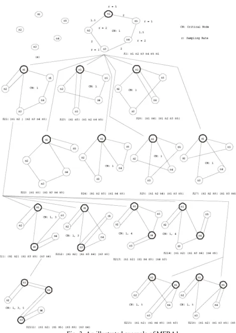
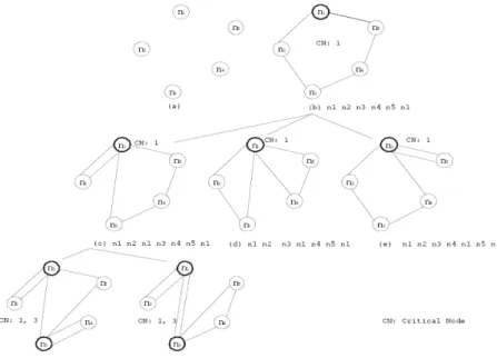
Consider the example in Fig. 3. There is a sensor network with a set of sensor nodes
N = {n1, n2, …, n5}. The sensing rate (r1, …, r5) = (5, 2, 1, 2, 1) and the buffer size (b1, b2,
b3, b4, b5) = (44, 44, 44, 44, 44). The distance between every pair of 5 sensors
0 1.5 3.4 2.6 2 1.5 0 2 2.3 2.5 [ ] 3.4 2 0 2 3.2 . 2.6 2.3 2 0 1.5 2 2.5 3.2 1.5 0 ij d ⎡ ⎤ ⎢ ⎥ ⎢ ⎥ ⎢ ⎥ = ⎢ ⎥ ⎢ ⎥ ⎢ ⎥ ⎣ ⎦
Assume that a message ferry with constant speed s = 1 to collect the sensing data. Applying phase 1, we find a least visiting sequence n1, n2, …, n5, n1, and a critical node
n1 (as shown in Fig. 3, state S1). In phase 2, start form critical node n1 and partition all
nodes {n1, n2, n3, n4, n5} into two sub-sets {{n1, n3}, {n1, n2, n4, n5}}, …, {{n1, n2, n5},
{n1, n3, n4}} (see states S21, S22, …, S27 in Fig. 3). Then, MFRA1 construct TSP sequence
Fig. 3. An illustrated example of MFRA1.
After executing steps 1 to 3 of phase 2, if there is not feasible solution, then we choose state S21 for further partition. Assume that there is another critical node n5 in {n1,
n3, n4, n5}, MFRA1 continues to partition the sequence {n1, n3, n4, n5} (see states S211,
S212, …, S216 in Fig. 3), construct the TSP sequence, and check the feasibility of the
se-quence.
After executing above steps, if there is another critical node n3 in sequence {n1, n3,
n5} in state S211, MFRA1 continues to partition the sequence {n1, n3, n5}, construct the
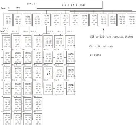
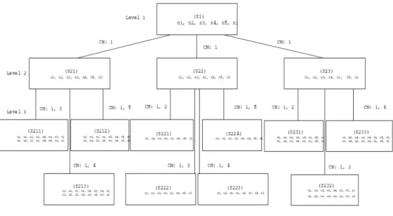
Fig. 4. The solution space of MFRA1 for the example.
Fig. 4 is the solution space for this illustrated example. Level 1 of Fig. 4 is the initial complete sequence. If all buffer size constraints are satisfied in level 1, then the solution is found. Otherwise, the least distance visit sequence is infeasible and search level 2 states. If all buffer size constraints are satisfied in any state of level 2, then the solution is found. Otherwise, search level 3 states, and so on. MFRA1 will stop after finding a fea-sible solution or checking all posfea-sible sequences. The following Lemma can help to speed up the search procedure.
Lemma 1 It is infeasible if partitioning critical node i leads node j to overflow and then partitioning node j leads critical node i to overflow in complete sequence k where 1 ≤ i, j ≤ m, i ≠ j, and m is the number of nodes.
Since TSP sequence is the shortest path, no other sequence has a path shorter than the TSP sequence. Therefore, it is infeasible if partitioning critical node i leads node j to overflow and then partitioning node j leads critical node i to overflow in complete se-quence k. 3.2 MFRA2
The MFRA1 algorithm can find the solution if the feasible solution exists. However, the MFRA1 is an exhaustive search and the computational time is untraceable. Thus, we
propose a heuristic algorithm, called MFRA2 which can find a solution more quickly. Details of the MFRA2 algorithm are illustrated as follows.
Phase 1:Find a least distance visit sequence
Phase 1 of MFRA2 is the same as phase 1 of MFRA1. Phase 2:Partition complete sequence
Start from a critical node, says ni1, partition the initial complete sequence ni1, ni2, …,
nim into sub-sequences in anti-clockwise direction, and check the feasibility of each
sen-sor node. Note that MFRA2 only generates m − 2 sequences ni1ni2ni1ni3…nimni1, ni1ni2ni3
ni1ni4…nimni1, …, ni1ni2…nim-1ni1nimni1 in the level one and check their feasibility. As shown in Fig. 5, a complete sequence n1n2n3n4n5n1 with one critical node n1 is partitioned into 3
sequences: n1n2n1n3n4n5n1, n1n2n3n1n4n5n1 and n1n2n3n4n1n5n1.
If all of the 3 sequences are infeasible, we choose one of them for further partition. For example, the sequence n1n2n1n3n4n5n1 with critical node n3 in sub-sequence n1n3n4n5n1 is
partitioned into two sequences n1n2n1n3n4n3n5n1 and n1n2n1n3n4n5n3n1 (see Fig. 5).
Fig. 5. An illustrated example of MFRA2.
An example of the solution space of MFRA2 is shown in Fig. 6. Level 1 of Fig. 6 is the initial complete sequence. If all buffer size constraints are satisfied in level 1, the solution is found. Otherwise, the initial complete sequence is infeasible and search level 2 states. If all buffer size constraints are satisfied in any state of level 2, the solution is found. Otherwise, search level 3 states, and so on. MFRA2 will stop after finding a fea-sible solution or checking all generated sequences.
Fig. 6. The solution space of MFRA2.
4. SIMULATION RESULTS
4.1 Performance Metrics and Environment Setup
This section presents the performance analysis of MFRA1 and MFRA2 algorithms. The environment setup of simulation is described as follows. There are different kinds of sensors such as surveillance sensors and data sensors in a two dimensional sensing area. The surveillance sensor has a high sampling rate to capture video message. Data sensor has a low sampling rate to collect temperature or noise data.
We study the following performance metrics.
(1) The travel time: The travel time of message ferry is defined as the time that message ferry goes through every node in the complete sequence.
(2) Number of sequences checked: The number of sequences checked is the number of sequences generated and feasibilities checked by the MFRA1 (or MFRA2) algorithm. (3) The amount of data lost: For a complete sequence (found by MFRA1, MFRA2,
Greedy algorithm, Nearest Neighbor, Lin Kernighan [20] or PBS [18]), we calculate the amount of data lost if the message ferry collects the data along this complete se-quence. The greedy algorithm finds a Hamiltonian cycle as a complete sequence greedily. The nearest neighbor algorithm constructs a Hamiltonian cycle as a com-plete sequence by starting at a node n0, choosing the nearest neighbor node as next
4.2 Numerical Results (1) The travel time
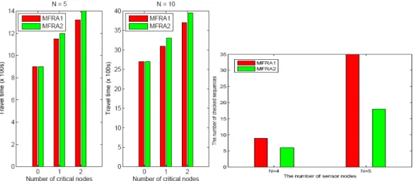
There are two set of sensors, (N = 5 and N = 10), in a 10 km × 10 km two-dimen- sional sensing field. The speed of the message ferry is 36 km/hr. The travel time vs. the number of critical nodes for MFRA1 and MFRA2 is shown in Fig. 7. Overall, the travel time increases when the number of critical nodes increases. This is because MFRA1 and MFRA2 continue to partition a sequence and the number of nodes in the resulting se-quence increases.
Fig. 7. The travel time vs. the number of critical nodes for MFRA1 (MFRA2) with 5 and 10 sensors.
Fig. 8. The number of checked sequences of MFRA1 and MFRA2 algorithms. (2) Number of sequences checked
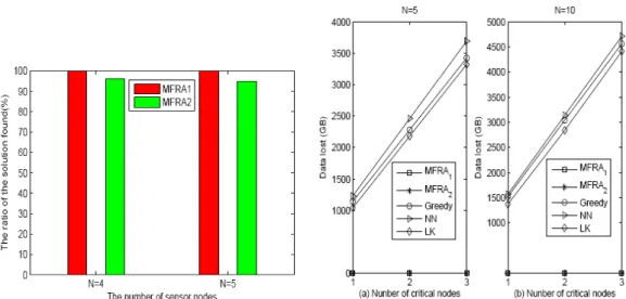
As shown in Fig. 8, the number of checked sequences of MFRA1 is much larger than MFRA2. This is because MFRA1 checks all sequences to find feasible solutions. MFRA1 algorithm can find the solution if the feasible solution exists. However, the MF- RA1 is an exhaustive search and it may consume lots of computation time. The MFRA2 is a heuristic algorithm and it can find a solution more quickly. But, the MFRA2 may not find the solution whenever the solution exists. This is because MFRA2 does not check all sequences. Fig. 9 shows the ratio of the solution found for MFRA1 and MFRA2. As shows in Fig. 9, the ratio of the solutions found of MFRA1 is nearly the same as MFRA2. Therefore, MFRA2 is an efficient algorithm.
(3) The amount of data lost
As shown in Fig. 10, the amount of data lost of MFRA1 and MFRA2 algorithms is much smaller than Greedy, Nearest Neighbor and Lin Kernighan algorithms. Greedy, Nearest Neighbor and Lin Kernighan algorithms will lose data when a sensor overflows. However, MFRA1 and MFRA2 work well without losing data. Fig. 11 shows the amount of data lost for different buffer sizes with 3 critical nodes. Fig. 12 shows the amount of
Fig. 9. The number of feasible solutions of MFRA1 and MFRA2 algorithms.
Fig. 10. The amount of data lost for different methods.
Fig. 11. The amount of data lost for different buffer sizes with 3 critical nodes.
Fig. 12. The amount of data lost for different buffer sizes with 2 critical nodes. data lost for different buffer sizes with 2 critical nodes. MFRA1 and MFRA2 perform better than other schemes.
5. CONCLUSIONS
This paper presents two efficient message ferry routing algorithms for data collec-tion in particollec-tioned wireless sensor networks. If there is a sensor overflow, MFRA1 and
MFRA2 fix the overflow by partitioning the initial visit sequence into some sub-se- quences to find feasible solutions. The partition phase of our scheme is the key difference compared to the previous schemes. It can achieve a better performance than other previ-ous schemes. MFRA1 and MFRA2 algorithms are efficient and novel for data collection in partitioned wireless ad hoc sensor networks.
REFERENCES
1. W. Zhao and M. Ammar, “Message ferrying: Proactive routing in highly partitioned wireless ad-hoc networks,” in Proceedings of the 9th IEEE Workshop on Future
Trends in Distributed Computing Systems, 2003, pp. 308-314.
2. W. Zhao, M. Ammar, and E. Zegura, “A message ferrying approach for data delivery in sparse mobile ad hoc networks,” in Proceedings of the 5th ACM International
Symposium on Mobile Ad Hoc Networking and Computing, 2004, pp. 187-198.
3. M. M. B. Tariq, M. Ammar, and E. Zegura, “Message ferry route design for sparse ad hoc networks with mobile nodes,” in Proceedings of International Symposium on
Mobile Ad Hoc Networking and Computing, 2006, pp. 37-48.
4. A. Vahdat and D. Becker, “Epidemic routing for partially connected ad hoc net-work,” Technical Report No. CS-200006, Department of Computer Science, Duke University, 2000.
5. W. Zhao, M. Ammar, and E. Zegura, “Controlling the mobility of multiple data tran- sport ferries in a delay-tolerant network,” in Proceedings of IEEE INFOCOM, 2005, pp. 1407-1418.
6. R. C. Suganthe and P. Balasubramanie, “Efficient routing for intermittently con-nected mobile ad hoc network,” International Journal of Computer Science and Net-
work Security, Vol. 8, 2008, pp. 184-190.
7. R. C. Suganthe and P. Balasubramanie, “Improving Qos in disconnected mobile ad hoc network,” Journal of Mobile Communication, 2008, pp. 99-104.
8. T. Spyropoulos, K. Psounis, and C. Raghavendra, “Efficient routing in intermittently connected mobile networks: The singlecopy case,” IEEE/ACM Transactions on
Net-working, Vol. 16, 2008, pp. 63-76.
9. T. Spyropoulos, K. Psounis, and C. Raghavendra, “Efficient routing in intermittently connected mobile networks: The multicopy case,” IEEE/ACM Transactions on
Net-working, Vol. 16, 2008, pp. 77-90.
10. Z. Zhang, “Routing in intermittently connected mobile ad hoc networks and delay tolerant networks: Overview and challenges,” IEEE Communications Surveys, 2006, pp. 24-37.
11. L. Pelusi, A. Passarella, and M. Conti, “Opportunistic networking: data forwarding in disconnected mobile ad hoc networks,” IEEE Communications Magazine, 2008, pp. 134-141.
12. A. A. Hanbali, M. I. Intria, V. Simon, E. Varga, and I. Carreras, “A survey of mes-sage diffusion protocols in mobile ad hoc networks,” in Proceedings of International
Conference on Performance Evaluation Methodologies and Tools, 2008, pp. 1-16.
13. W. Zhao, M. Ammar, and E. Zegura, “Controlling the mobility of multiple data trans- port ferries in a delay-tolerant network,” in Proceedings of IEEE INFOCOM, 2005,
pp. 1407-1418.
14. R. Viswanathan, J. Li, and M. Chuah, “Message ferrying for constrained scenarios,” in Proceedings of the 6th IEEE International Symposium on World of Wireless
Mo-bile and Multimedia Networks, 2003, pp. 487-489.
15. M. Chuah and P. Yang, “A message ferrying scheme with differentiated services,” in
Proceedings of IEEE MILCOM, 2005, pp. 1521-1525.
16. R. C. Shah, S. Jain, and W. Brunette, “Data MULEs: Modeling a three-tier architec-ture for sparse sensor networks,” in Proceedings of the 1st IEEE International Work-
shop on Sensor Network Protocols and Applications, 2003, pp. 30-41.
17. A. A. Somasundara, A. Ramamoorthy, and M. B. Srivastava, “Mobile element sched- uling for efficient data collection in wireless sensor networks with dynamic dead-lines,” in Proceedings of the 25th IEEE International Real Time Systems Symposium, 2004, pp. 296-305.
18. Y. Gu, D. Bozdağ, E. Ekici, F. Ozgüner, and C. G. Lee, “Partitioning based mobile element scheduling in wireless sensor networks,” in Proceedings of the 2nd Annual
IEEE Communications Society Conference on Sensor and Ad Hoc Communications and Networks, 2005,pp. 386-395.
19. D. Applegate, R. E. Bixby, V. Chvatal, and W. Cook, “On the solution of traveling salesman problems,” Documenta Mathematica, Extra Volume ICM III, 1998, pp. 645- 656.
20. S. Lin and B. W. Kernighan, “An effective heuristic algorithm for the traveling sales- man problem,” Operation Research, 1973, pp. 498-516.
Jyh-Huei Chang (張志輝) received his M.S. degree in Com- puter Science from National Chiao Tung University, Taiwan in 2002. He is currently working toward the Ph.D. degree in Com-puter Science at National Chiao Tung University, Taiwan. He is a Ph.D. candidate now. His research interests include wireless net- works, wireless sensor networks and mobile computing.
Rong-Hong Jan (簡榮宏) received the B.S. and M.S. de-grees in Industrial Engineering and the Ph.D. degree in Computer science from National Tsing Hua University, Taiwan, in 1979, 1983, and 1987, respectively. He joined the Department of Com- puter and Information Science, National Chiao Tung University, in 1987, where he is currently a professor. From 1991-1992, he was a visiting associate professor in the Department of Computer Science, University of Maryland, College Park, Maryland. His research interests include wireless networks, mobile computing, distributed systems, network reliability, and operations research.