助聽器回授路徑測量及適應性的噪音消除演算法

國

立

交

通

大

學

電子工程學系 電子研究所碩士班

碩

士

論

文

助聽器回授路徑測量及適應性的噪音消除演算法

Measurement of feedback paths and adaptive

noise cancellation algorithms in hearing aids

研 究 生：陳 建 男

指導教授：桑 梓 賢 教授

助聽器

回授路徑測量及適應性的噪音消除演算法

Measurement of feedback paths and adaptive noise

cancellation algorithms in hearing aids

研 究 生：陳建男 Student：Chien-Nan Chen

指導教授：桑梓賢 教授 Advisor：Tzu-Hsien Sang

國 立 交 通 大 學

電子工程學系 電子研究所碩士班

碩 士 論 文

A Thesis

Submitted to Department of Electronics Engineering & Institute of Electronics College of Electrical and Computer Engineering

National Chiao Tung University in Partial Fulfillment of the Requirements

for the Degree of Master

in

Electronics Engineering September 2009

Hsinchu, Taiwan, Republic of China

中 華 民 國 九 十 八 年 九 月

助聽器回授路徑測量及適應性的噪音消除演算法

研究生：陳建男 指導教授：桑梓賢 教授

國立交通大學

電子工程學系 電子研究所碩士班

摘要

本篇論文主要探討助聽器回授路徑(feedback path)的測量及使用適應性濾波器 (adaptive filter)消除噪音的演算法模擬。 我們首先用一個耳內型(ITC)助聽器，裡面無放大電路僅有接收器(receiver)及麥克 風(microphone)，接上脈衝產生器(pulse generator)使用掃頻(sweep stimulus)的方式驅動 助聽器的接收器並接收麥克風的聲音得到回授路徑的頻率響應(frequency response)，再 由程式將之轉回時域的脈衝響應(impulse response)，我們的測量結果可供消除回授演 算法的參考及實現。 卡爾曼濾波器(Kalman filter)是一種有效率的適應性濾波器且可應用在時變系統 上。尤其是更新估記狀態時僅需計算前一個狀態估記值及新得到的資料，所以只有前 個狀態需要儲存。因此我們考慮將卡爾曼濾波器列入助聽器消除噪音演算法的可能 性。我們做了一些卡爾曼濾波器在單一頻帶消除白雜訊的學習，至於在分頻濾波上加 上卡爾曼濾波器因為可能增加大量運算故先暫時予以保留。

Measurement of feedback paths and adaptive noise

cancellation algorithms in hearing aids

Student：Chien-Nan Chen Advisor：Tzu-Hsien Sang

Department of Electronics Engineering & Institute of Electronics

National Chiao Tung University

ABSTRACT

In this thesis, we focus on the measurement of feedback path of hearing aids and the simulation of adaptive filter algorithm for noise cancellation.

First of all we put an ITC hearing aid embodying only a receiver and a microphone in the artificial ear in the anechoic chamber. We use the pulse generator to inject the sweep signal to the receiver and receive the sound from the microphone to get the frequency response. Then make use of Matlab to transform it into impulse response. Our measurement result may supply to the realization of the feedback cancellation algorithm.

Kalman filter is an efficient adaptive filter and can be used for time-varying system. It only needs the estimated state from the previous time step and the current measurement to

Therefore we consider the possibility of using the Kalman filter in hearing aids for noise cancellation. The single-band Kalman filter for white noise cancellation is studied while the multi-band Kalman filter is kept aside due to the possible surge in computational cost.

誌謝

首先要感謝我的指導教授-桑梓賢老師，謝謝老師給我很多研究方向的啟發，也從 老師身上學到很多學業外的經驗及智慧，真的很感謝老師不吝辛苦的指導，才有這篇 論文的完成。再來要感謝我的父母給我的支持及鼓勵，謝謝他們從小到大無怨無悔地 照顧我，讓我無後顧之憂得專心在課業上。 接者要感謝科林助聽器及工程師林權宜先生，在我們助聽器的維修上麻煩他們許 多。在測量回授路徑的問題上要感謝機械系白明憲老師及其學生王俊仁同學借我們無 響室及許多實驗儀器，在測量方面也教導我們很多，實在萬分感謝。另外也要感謝助 聽器計劃的誠文學長、政君、羽庭、韋廷、永昌等每個實驗室學長及同學們的指教及 包涵。 感謝實驗室的學長欣德、正湟在研究上給我很多建議及指導，還要謝謝實驗室同 學宇峰、俞榮及學弟們譯賢、宗達、哲聖、耀賢、旭謙、俊育陪我度過很愉快且充實 的研究所生活，謝謝大家。 建男 2009.10.5

Contents

Chapter 1 Introduction ... 1

1.1 Overview of hearing aids ... 1

1.2 Introduction to hearing aid systems ... 3

Chapter 2 Measurement of feedback paths in hearing aids ... 7

2.1 Introduction to the feedback path ... 7

2.2 ITC digital hearing instrument... 9

2.3 Sweep stimulus method... 11

2.4 Modeling the EFP in the time-domain... 15

Chapter 3 Adaptive noise cancellation algorithms in hearing aids ... 17

3.1 Introduction ... 17

3.2 Kalman filtering for white noise cancellation... 19

3.3 Simulation ... 22

3.4 Discussion... 30

Chapter 4 Conclusions and future work ... 33

4.1 Conclusions ... 33

4.2 Future work ... 34 Bibliography 35

List of Figures

Fig. 1.1 Some types of hearing aids ... 3

Fig. 1.2 Block diagram of a digital hearing aid ... 4

Fig. 2.1 Block diagram of the basic hearing instrument system with adaptive feedback cancellation. ... 9

Fig. 2.2 Experimental setup with the ITC placed in-situ... 10

Fig. 2.3 Experimental system to measure the EFP. ... 11

Fig. 2.4 Frequency response of EFP ... 12

Fig. 2.5 Frequency response of the closed-loop ... 13

Fig. 2.6 Frequency response of the acoustic feedback path ... 14

Fig. 2.7 Frequency response of the closed-loop ... 14

Fig. 2.8 Impulse response of the EFP ... 16

Fig. 3.1 The flowchart of the frame-based AR Kalman filtering for white noise cancellation ... 21

Fig. 3.2 The flowchart of the fixed AR Kalman filtering for white noise cancellation ... 21

Fig. 3.3 Time plot of enhanced SNR-5 white noisy speech by frame-based AR4 Kalman filtering. ... 23 Fig. 3.4 Spectrogram of enhanced SNR-5 white noisy speech by frame-based

Fig. 3.5 Time plot of enhanced SNR-5 white noisy speech by fixed AR4 Kalman

filtering ... 24

Fig. 3.6 Spctrogram of enhanced SNR-5 white noisy speech by fixed AR4 Kalman filtering ... 24

Fig. 3.7 SNRseg of speech frames for frame-based AR Kalman filtering ... 25

Fig. 3.8 PESQ of speech frames for frame-based AR Kalman filtering ... 26

Fig. 3.9 SNRseg of speech frames for fixed AR Kalman filtering ... 27

Fig. 3.10 PESQ of speech frames for frame-based AR Kalman filtering ... 28

Fig. 3.11 PESQ of sentences in different SNR0 speech samples ... 29

List of Tables

Table 3.1 SNRseg of speech frames for frame-based AR Kalman filtering ... 25

Table 3.2 PESQ of speech frames for frame-based AR Kalman filtering ... 26

Table 3.3 SNRseg of speech frames for fixed AR Kalman filtering ... 27

Table 3.4 PESQ of speech frames for fixed AR Kalman filtering ... 28

Table 3.5 Overall complexities of a Kalman filter ... 31

Table 3.6 Complexities of Kalman filtering and spectrum subtracton for white noise cancellation... 31

Chapter 1

Introduction

1.1 Overview of hearing aids

Tremendous improvements have been realized in recent years in the technology to assist and improve human hearing. This is especially evident in advances in computers and subsequent miniaturization of manufacturing. In the past, hearing aids simply amplified sound, i.e. made it louder across the board. But the fact that every person has a different hearing profile prevent the flat-amplification approach unsuitable for most cases.

The older hearing aids couldn't adjust from one type of sound to another; they just made all the sounds louder. While that might have helped people hear some sounds they wanted to hear, they also amplified unwanted sounds that became uncomfortable.

Older technology lacks the flexibility and adaptability of nowadays state-of-art technologies, especially those enabled by the advance of computing power and micro-electronics. Today's hearing instruments actively process sound and match it specifically to individual hearing needs. These instruments take the incoming sound, analyze it with their digital micro-processors, adjust, shape and convert it into the type of sound according to the customized hearing-loss compensation profiles with high accuracy. It is therefore possible to realize many acoustic and speech processing methods which

simply existed on paper but were not available in hearing aids simply because of the complexity of implementation; the advance in hardware also opens new opportunities to develop even more sophisticate signal processing approaches that were not imaginable just a decade ago.

Today’s hearing-loss compensation strategy aims to amplify sound separately for each frequency bands, according to the degree of hearing loss. Therefore the entire sound is not amplified with a flat gain, but only that bands with severe hearing loss are subjected to high-level amplification. This method allows the hearing instrument to be tuned to the frequencies where the hearing loss specifically requires assistance. It does this by actually "shaping" the sound in the frequency domain specifically to suit the patient’s needs and by keeping it within the comfort range.

The most advanced hearing instruments today have multi-memory capabilities that change with the listening environment. Some do this automatically, some with the push of a button on the instrument, and some with a remote control. Some also have directional microphones that effectively reduce the background noise and enhance speech intelligibility.

Other advantages in today's hearing instruments are that they are smaller, more flexible and better able to deal with background noise. Here are some types of hearing aids shown in Fig. 1.1 [29].

Fig. 1.1 Some types of hearing aids [29].

1.2 Introduction to hearing aid systems

The number of hearing impaired individuals who need to use hearing aids is rapidly increasing [1]. But the cost of hearing aids is still a big concern for those in need. The goal of the NCTU hearing-aid team is to develop a low cost and low power-consumption, but yet high-performance hearing aid. It is therefore very important to consider signal processing tasks in terms of ease of implementation and power consumption in addition to effectiveness. In the following, the basic structure of hearing-aids is presented; along the way, major issues and signal processing tasks will be discussed and the main theme of this thesis will become clear.

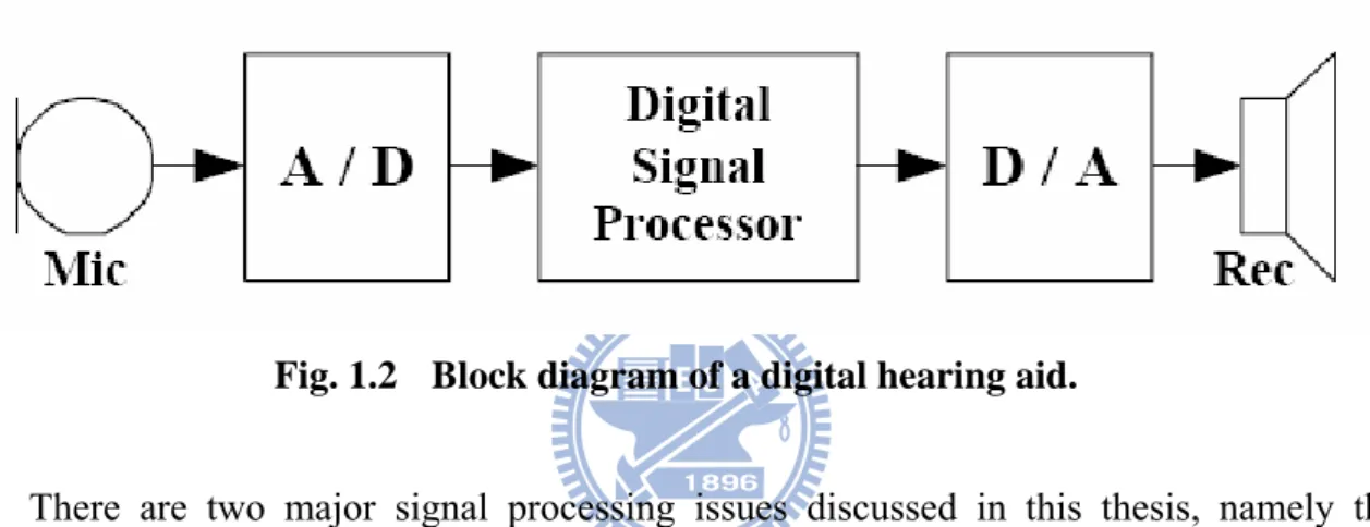
Current hearing aids are digital devices that embody input (microphone) and output (receiver/subminiature loudspeaker) transducers, analog input conditioning circuits, an analog-to-digital converter (ADC), a digital signal processor (DSP), a digital-to-analog converter (DAC) and a power amplifier [2]. The block diagram of a digital hearing aids is shown in Fig. 1.2. Hearing aids amplify incoming sound according to the hearing-loss profile of the patient so as to increase the signal level and compensate part of the hearing loss.

Fig. 1.2 Block diagram of a digital hearing aid.

There are two major signal processing issues discussed in this thesis, namely the feedback problem and the noise reduction problem. First, consider the feedback problem. Due to imperfect earmold fitting and venting in the hearing aid device, there is acoustic leakage from the receiver to the microphone. The leakage causes a regenerative feedback loop, which frequently makes the hearing aid oscillate and results in a whistling sound. For people with severe hearing loss, this problem is serious because at high gains there is an increased risk of squealing which may render the hearing aid useless. Feedback becomes more apparent when an object is close to the ear (i.e. when using a telephone) or when the jaw is moving (i.e. when chewing). In case of squealing, hearing aid users tune down the hearing aid gain or fit hearing aids more tightly in the ear canal, but such adjustments may compromise the function and comfort of the hearing aid [3].

To solve the problem of feedback, modern hearing-aids usually utilize adaptive filtering to imitate and eliminate the feedback signal. But before doing that, knowledge about typical feedback path is essential in making specifications on the adaptive feedback canceling filter. The first contribution of this thesis therefore consists of establishing an acoustic measuring environment and carrying out feedback path measurement and estimation task. An ITC hearing-aid earmold embodied with a receiver and a microphone, together with an artificial ear in the acoustic chamber, is used in the experiment. More technical details can be found in Chapter two. Our measurement results provide a reference point for the specification and implementation of the feedback canceling filter.

The second major issue is the background noise experienced in the daily lives of hearing aid users; this greatly reduces the speech intelligibility as well as comfort of listening [4]. Quite often noise reduction is a built-in feature for modern hearing aids, especially when the users’ primary need is to comprehend human speech. To achieve effective reduction, the usual approach is first to identify the defining characteristics of the speech and non-speech signals, then do different operations to signals with different characteristics. Not surprisingly, the most common operation is filtering.

In Chapter three, we consider the possibility of using the Kalman filter in hearing-aids for noise reduction. The single-band Kalman filter is studied while the multi-band Kalman filter is kept aside due to the possible surge in computational cost. We did simulation and comparison studies between the Kalman filter and the well-known spectrum subtraction method. The Kalman filter, in general, has the potential of obtaining better performance in reducing the noise, while the spectral subtraction method enjoys simple formulation and easy implementation. In considering signal processing tasks for real-time applications like hearing-aids, it is important to keep in mind that performance evaluation is not always the

major criterion of choosing particular signal processing algorithms. Easy implementation and low consumption, which often come with the low computation cost, are rather important, if not more important, in making the decision. We also suggest the possibility of combining the Kalman filter and the existing analysis/synthesis filter bank as the future development in order to achieve a balance between the performance and low power/cost.

Chapter 2

Measurement of feedback paths in

hearing aids

2.1 Introduction to the feedback path

Undesirable acoustic feedback is an uncomfortable squeal that occurs when the output sound from the receiver leaks to the microphone and that leaked sound gets re-amplified. Unstable acoustic feedback develops into a problem when the earmold/earshell is loosely fitted (or a large vent is part of the earmold/earshell) and when there is large signal amplification in the hearing instrument. From a signal processing viewpoint, this feedback mechanism is usually modeled as a linear operation and typical system identification methods are used to obtain the feedback path model.

The most straightforward method to reduce the possibility of unstable acoustic feedback is to reduce the gain, but this is often unacceptable because reducing gain means that the effectiveness of hearing-aids would be severely limited. To maintain the amplifying gain while prevent the onset of unstable acoustic feedback, many modern hearing instruments feature adaptive feedback canceling algorithms. Among them the popular methods include adaptive notch filters, automatic gain reduction in a multi-channel system and several variations of adaptive feedback cancellation [4],[5]. Of these, the adaptive

feedback cancellation methods that estimate the feedback path and subtract it from the input signal of the hearing instrument are arguably the most effective to date. From a clinical perspective, although many manufacturers claim an increased gain of ≧15dB (with the application of these algorithms) before the onset of unstable acoustic feedback , an increased gain of ＜10dB is often the case.

The hearing instrument system, in particular the acoustic feedback path, has been studied, especially been modeled as a linear system depicted in Fig. 2.1. For example, Lybarger [6] measured the frequency response, but the frequency response was limited only to magnitude responses at a few selected frequencies. Bustamante [5] chose click sequences as stimuli and measured the response. The impulse response of the system was calculated by averaging the responses. Stinson [7] measured the frequency response with a sweep stimulus. Egolf et al. [8] modeled each component of a glass type analog hearing instrument by two-port methods that took load effects into consideration. Kates [9] transferred each component of an ITE hearing instrument from frequency domain into time domain that matched the magnitude response, but ignored the phase response. Jingbo Yang [2] used sweep stimulus and white noise method to model the EFP in an ITE hearing instrument and verify the Nyquist criterion. Then he employed an adaptive LMS FIR filter to determine the impulse response of the EFP.

In this chapter, we describe a measuring platform to facilitate research for the development of acoustic feedback algorithms. Specially we consider the magnitude and phase response of the external feedback path (EFP) obtained by the sweep stimulus method. Using the characteristics of EFP obtained, we predict theoretically (Nyquist criterion) the

impulse response. An adaptive Finite-Impulse-Response (FIR) filter can be used to match the actual EFP impulse response such that the effects of the EFP can be nullified (Fig. 2.1) [2].

Fig. 2.1 Block diagram of the basic hearing instrument system with adaptive feedback cancellation [2].

2.2 ITC digital hearing instrument

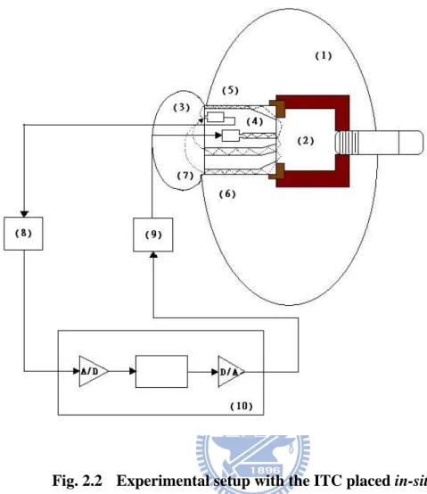
In this section, we will describe the experimental setup of the measurement platform. The hearing instrument used in this setup is a custom-made In-The-Canal (ITC) hearing instrument embodying only a microphone and a receiver. The block diagram is shown in Fig. 2.2.

Fig. 2.2 Experimental setup with the ITC placed in-situ.

Legend

(1) Artificial head (Head and Torso Simulator-Type 4128C) (2) Artificial right ear (Head and Torso Simulator-Type 4128C) (3) Artificial pinna (Head and Torso Simulator-Type 4128C) (4) ITC hearing instrument shell with a microphone and receiver (5) Knowles FG-23742-D36 microphone

(6) Knowles FK-23451-000 receiver (7) Acoustical feedback path

(8) Interface between microphone and ADC (9) Interface between DAC and receiver (10) PC, B&K3560-C

2.3 Sweep stimulus method

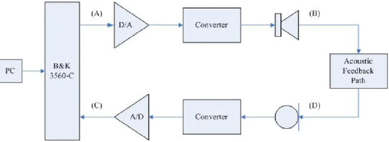
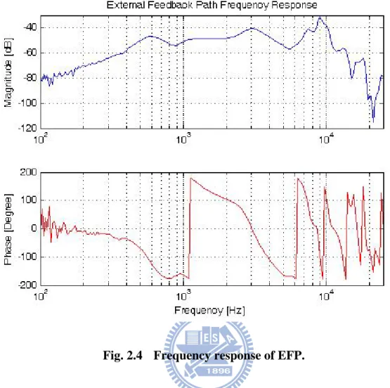
The method we used to obtain the frequency response of the EFP is called the sweep stimulus method. In the method, a sweep signal (its frequency changes from low to high) is utilized as the stimulus to the receiver. The sinusoidal sweep signal 1volt(rms) from 100Hz to 25000Hz is injected into (A) and the output of (C) is measured. In general hearing aids just consider the frequency bandwidth which is from 200Hz to 8000Hz. But in our experiment we measure the frequency response from 100Hz to 25000Hz to obtain the broader result and get a better impulse response. We depict the signal flow of the measurement platform in Fig. 2.3. The stimulus sweep signal is obtained from the pulse generator (B&K 3560C). Because the microphone in the hearing aid is unstable above 10000Hz, we use another microphone (B&K4190L) put near the hearing aid’s microphone to measure the feedback path from 100Hz to 25000Hz. By means of the platform, we obtain the sound pressure level of EFP. Then we transfer it to voltage and then depict the frequency response in Fig. 2.4.

Fig. 2.4 Frequency response of EFP.

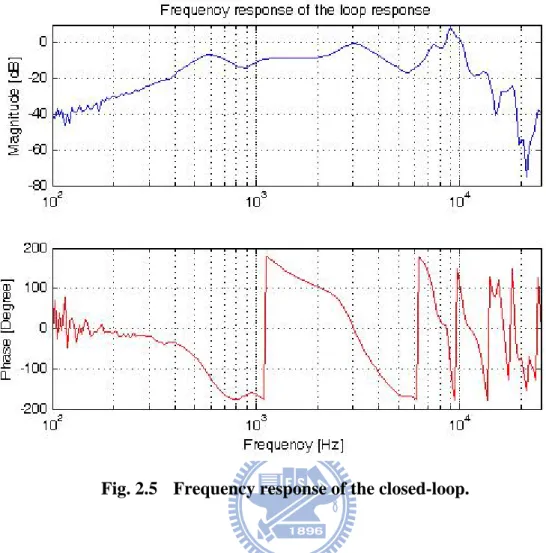
The Nyquist criterion states that oscillations will occur if the magnitude response of the loop-gain is greater than unity and the phase response is a multiple of 2π. Most hearing aids have different gains in different frequency. Usually the maximum gain is above 40dB. Therefore we suggest the gain of our hearing aid system is a constant. So we plus the gain 40dB and get the closed-loop response as Fig. 2.5. Therefore in our system the oscillations may occur in 3000Hz and 9000Hz. As a result, the howling may occur in 3000Hz in a general hearing aid.

Fig. 2.5 Frequency response of the closed-loop.

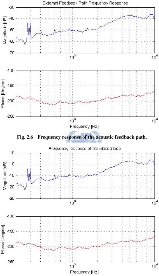
On the other hand, we also used the hearing aid microphone and the microphone in right ear simulator to model the acoustic feedback path which is equivalent to the transfer function from (B) to (D) in Fig. 2.3. We assume that the sound pressure level in ear canal is almost the same as that of the receiver. So the SPL of hearing aid divided by that of the ear canal is equivalent to the transfer function of the acoustic feedback. The frequency response of the acoustic feedback path is as Fig. 2.6. We also give it a 40dB gain to obtain the closed-loop response which is as Fig. 2.7. Therefore the hearing aid may oscillate in 6200Hz.

2.4 Modeling the EFP in the time-domain

In the previous section, we have modeled the frequency response of the EFP with sweep stimulus. As most of the recent feedback cancellation methods are based on adaptive filtering ( the filter response changes with time according to the variance of the EFP ), it is imperative to model the EFP in the time domain. The time-domain model proposed by Kates [9], as mentioned earlier, considered only the magnitude response and ignored the phase response. However, as we have shown in the previous section, the phase of the EFP is important for determining the frequency where acoustic oscillation occurs.

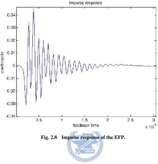
To determine the impulse response of the external feedback path, we employed a Matlab program which uses the IFFT function to transfer the frequency response to the time-domain that is impulse response. In order to get a more natural impulse response, we took the broadband frequency response as Fig. 2.4 to deal with. The impulse response is depicted in Fig. 2.8. And we can obtain the feedback time which is about 3 milliseconds (ms). As a result , the processing time of feedback cancellation should be in 3 ms. Therefore the time-domain model (or impulse response) can therefore be used for the development of acoustic feedback cancellation algorithms in the future.

Chapter 3

Adaptive noise cancellation

algorithms in hearing aids

3.1 Introduction

Noise problem naturally arise in many areas, such as voice communication, speech recognition, and hearing aids. As a result, noise cancellation becomes an important research topic and many studies have been using techniques such as short-time spectral amplitude estimation [10]-[13], iterative Wiener filtering [14]-[16], audio-based filtering [17],[18], signal-subspace processing [19],[20], and hidden Markov modeling (HMM) [21],[22]. Although significant results have been achieved, most of them are not suitable for real-time implementation because their computational complexities are generally too high.

The Kalman filter is well known in signal processing for its efficient structure, and it can be used for time-varying system. It is used in a wide range of engineering applications from radar to computer vision, and is an important topic in control theory and noise cancellation. The Kalman filter is a recursive estimator, that is to say, it only needs the estimated state from the previous time step and the current measurement to estimate the current state. Since it has the potential of high performance, is naturally adaptive, and may qualify for low computational cost, we decided to study the possibility of applying it to noise cancellation in hearing aids.

In [23], Paliwal and Basu used a Kalman filter to enhance speech corrupted by white noise. On a short-time base, speech signals were modeled as stationary AR process and AR parameters were assumed to be known. Gibson, Koo, and Gray considered speech enhancement with colored noise in [24]. They modeled both speech and colored noise as AR processes and developed scalar and vector Kalman filtering algorithms. To estimate the AR coefficients, an EM-based algorithm was employed. In [25], Lees and Ann proposed a non-Gaussian AR model for speech signals. They modeled the distribution of the driving-noise as a Gaussian mixture and applied a decision-directed nonlinear Kalman filter. Again, an EM-based algorithm was used to identify unknown parameters. Niedzwiecki and Cisowki [26] assumed that speech signals are nonstationary AR processes and used a random-walk model for the AR coefficients. An extended Kalman filter was then used to simultaneously estimate speech and AR coefficients, Note that the stability of the extended Kalman filter is not guaranteed and dimensions of the Kalman filter are greatly increased.

The aforementioned Kalman filtering algorithms still require extensive computations for two reasons: first, using EM algorithms to identify AR coefficients costs a lot, and second, using Kalman filters usually involves matrix inversion. However, the above costs depend on the order of the Kalman filter used. In order to carefully assess the pros and cons of using Kalman filters in hearing aids, we intend to use low-order Kalman filters and low-cost Yule-Walker method for estimating AR coefficients. As a future plan, Kalman filters incorporating with sub-band filtering structure will also be studied; in this case, zero or first-order Kalman filters may be sufficient and the calculation only involves scalar operations, thus saving a considerable amount of computation [27].

3.2 Kalman filtering for white noise cancellation

We derived the following from [27],[24]. On a short-time basis, a speech sequence ( )n

x can be represented as an AR process, which is essentially the output of an all-pole

linear system driven by a white noise sequence: 1 ( ) ( ) ( ) p i i x n a x n i w n = =

∑

− + (3.1) where ( )w n is a zero-mean white Gaussian process with variance σ_w2. The observed

speech signal z n is assumed to be contaminated by a zero-mean additive Gaussian ( ) noise v n( ) , i.e., z n

( )

=x n

( ) ( )

+v n . Let v n( ) be white and

( ) [ ( ) ( 1) ( 1)]T

n x n x n x n p

Δ

= − ⋅⋅⋅ − +

x . Equation (3.1) and the corrupted speech ( )z n can be

formulated in the state-space domain as

( ) ( 1) T ( ) n = n− + w n x Fx H (3.2) ( ) ( ) ( ) z n =Hx n +v n (3.3) 1 2 1 1 0 0 0 0 1 0 0 0 0 1 0 p p p p a a a ₋ a × ⋅ ⋅ ⋅ ⎡ ⎤ ⎢ _{⋅ ⋅ ⋅} ⎥ ⎢ ⎥ ⎢ ⋅ ⋅ ⋅ ⎥ ⎢ ⎥ = ⋅_⎢ ⋅ ⋅ ⋅ ⋅ _⎥ ⎢ _{⋅ ⋅ ⋅ ⋅ ⋅} ⎥ ⎢ ⎥ ⋅ ⋅ ⋅ ⋅ ⋅ ⎢ ⎥ ⎢ _{⋅ ⋅ ⋅} ⎥ ⎣ ⎦ F (3.4) 1 [10 00]×p = ⋅⋅⋅ H (3.5)

From standard Kalman filtering theory for white message and measurement noise, the state vector estimate is

With the initial condition xˆ(0)=0. The gain and error covariance equations are _{( )= ( ) [ ( ) + ]}−1 R n n n M HT HM HT G (3.7) M(n)=FS(n−1)FT +HTQH (3.8) S(n)=[I−G(n)H]M(n) (3.9) where G(n)is the Kalman gain vector, M(n)is the prediction-error covariance matrix,

) (n

S is the filtering-error covariance matrix, R=σ_v2 is the variance of the noise

sequence{ nv( )}, and Q=σ_w2 is the variance of the driving term{ nw( )}. With the initial

condition, S(0)= ][0 p×p, (3.8) is processed first, followed by (3.7) and (3.9). The speech

sample estimate at time instant n is finally obtained by xˆ(n)=H ˆx. The parameters

1 [a a_p] Δ

=

a _L and σ_w2 are computed over block lengths of 360 samples using the

autocorrelation method from the noisy observations when the true values are not known. The frame length of 360 samples corresponds to 15ms and was selected arbitrarily from within the common parameter update range of 10 to 30 ms often used in linear predictive systems. The frame length is not critical to the filter performance within these bounds. The noise variance 2

v

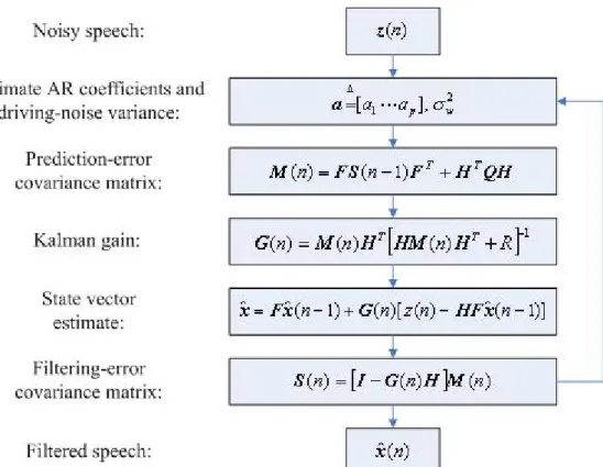
σ is estimated in some time interval before speech is present. Fig. 3.1 is the flowchart of the Frame-based AR Kalman filtering for white noise cancellation. At each iteration, we alternately estimate the parameters and filter the speech.

For the complexity of estimating AR coefficients, we propose a simpler method to reduce the computation of AR coefficients. First we estimate the AR coefficients from a clean speech, and then we use the Kalman filter with the fixed AR coefficients to filter the noisy speech. Fig. 3.2 is the flowchart of the fixed AR Kalman filtering for white noise cancellation. We reduce the computation and get a not bad performance in Kalman filtering for white noise cancellation. The simulation results are listed in section 3.3.

Fig. 3.1 The flowchart of the frame-based AR Kalman filtering for white noise cancellation.

3.3 Simulation

In this section, we take a girl’s sound “girl , meat ball” in Mandarin from Hearing and Speech Engineering Lab in National Yang-Ming University to be the clean input speech. This sentence of sound is sampling in 24KHz and about 3.2sec. The white noise we used is a function “rand” in Matlab. We add the white noise in some level of SNR and used the Kalman filter to enhance the noisy signal. Here are some simulation results and we will discuss them in the next section.

In the frame-based AR method we estimate AR coefficients and filter speech in every frame. Fig. 3.3 and Fig. 3.4 are the plots of frame-based method. Then we evaluate the SNRseg and PESQ of speech frames in Table 3.1 and Table 3.2 in different AR orders and in different SNR. Differently we estimate the AR coefficients once from the clean sentence and filter the noisy sentence with the fixed AR coefficients. Then we have the simulation plots of fixed AR method in Fig. 3.5 and Fig. 3.6. After that we also construct Table 3.3 and Table 3.4 with evaluation of speech frames in different AR orders and in different SNR.

Finally we also take five girl’s speech samples from Hearing and Speech Engineering Lab in National Yang-Ming University to be the clean input speech. We contaminate the five speech samples in SNR0 and evaluate those PESQ as the benchmark. Then we use the fixed AR method and framed-base AR method in AR order 4 to enhance these noisy speeches. The simulation results are as Fig. 3.11 and Fig. 3.12.

Fig. 3.3 Time plot of enhanced SNR-5 white noisy speech by frame-based AR4 Kalman filtering.

Fig. 3.4 Spectrogram of enhanced SNR-5 white noisy speech by frame-based AR4 Kalman filtering.

Fig. 3.5 Time plot of enhanced SNR-5 white noisy speech by fixed AR4 Kalman filtering.

Table 3.1 SNRseg of speech frames for frame-based AR Kalman filtering. Order\SNR -5 0 5 10 15 Noisy 6.11 11.02 15.99 20.99 25.94 AR1 8.63 13 17.37 21.87 26.42 AR2 9.73 14.2 18.66 23.05 27.32 AR3 10.05 14.47 18.85 23.22 27.49 AR4 10.17 14.56 18.93 23.29 27.52 5 10 15 20 25 ‐5 0 5 10 15 SNRseg SNR Noisy AR1 AR2 AR3 AR4

Table 3.2 PESQ of speech frames for frame-based AR Kalman filtering. Order\SNR -5 0 5 10 15 Noisy 1.91 2.2 2.42 2.69 2.97 AR1 1.94 2.21 2.44 2.72 3 AR2 1.98 2.25 2.49 2.77 3.04 AR3 2.01 2.28 2.51 2.8 3.07 AR4 2.01 2.29 2.52 2.81 3.07 1.8 2 2.2 2.4 2.6 2.8 3 ‐5 0 5 10 15 PESQ SNR Noisy AR1 AR2 AR3 AR4

Table 3.3 SNRseg of speech frames for fixed AR Kalman filtering. Speech -5 0 5 10 15 Noisy 6.11 11.02 15.99 20.99 25.94 AR1 9.05 12.75 16.75 21.25 26.03 AR2 11.52 15.55 19.58 23.49 27.3 AR3 12.39 16.06 19.72 23.6 27.57 AR4 12.67 16.09 19.77 23.69 27.59 5 10 15 20 25 1 2 3 4 5 SNRseg SNR Noisy AR1 AR2 AR3 AR4

Table 3.4 PESQ of speech frames for fixed AR Kalman filtering. Order\SNR -5 0 5 10 15 Noisy 1.91 2.2 2.42 2.69 2.97 AR1 2.04 2.27 2.46 2.71 2.98 AR2 2.13 2.36 2.6 2.83 3.03 AR3 2.2 2.48 2.67 2.84 3.05 AR4 2.31 2.51 2.68 2.86 3.05 1.8 2 2.2 2.4 2.6 2.8 3 ‐5 0 5 10 15 PESQ SNR Noisy AR1 AR2 AR3 AR4

1.5 1.6 1.7 1.8 1.9 2 2.1 2.2 2.3 2.4 2.5 0 1 2 3 4 5 6 PESQ different speech Noisy Fixed Frame

Fig. 3.11 PESQ of sentences in different SNR0 speech samples.

1.5 1.7 1.9 2.1 2.3 2.5 0 1 2 3 4 5 6 PESQ different speech Noisy Fixed Frame

3.4 Discussion

From Table 3.1 to Table 3.4 we can find that SNRseg and PESQ are directly proportional to AR order. Intuitively, cleaner speech signals generate more accurate estimates of AR coefficients. Therefore we can model the speech signal more accurately. In these examples the SNRseg and PESQ grades of the two methods saturate on AR3. In my experience different noisy speech signals saturates on different AR orders. Generally AR4 is good enough to model the speech signals.

In Fig. 3.11 and Fig. 3.12 we contaminate five different speech samples and use the two methods to enhance them. Obviously in speech sample 1 and 3 the fixed AR method is much better than frame-based method. On the other hand the frame-based method is better in the other speech samples. Generally the two methods can enhance noisy speech except the few samples. For example in speech sample 4 the fixed AR method’s PESQ is worse than unfiltered noisy speech. But in the subjective evaluation of speech quality, the filtered speech still sounds better than the unfiltered noisy speech does. Since PESQ is an objective measure to simulate the evaluation of the subjective speech quality, it is a valuable reference but not an absolute standard. In order to further compare the significant difference in speech quality resulting from these algorithms, we should do the subjective listening tests [31].

In this part, we discuss the computational complexities of Kalman filtering. The following result is derived from [27]. First, we define three terms for measuring complexity: MPU, multiplications per unit of time; DVU, divisions per unit of time; and APU, additions per unit of time. According to (3.1), speech is modeled as AR(p). If p≥ the AR 1

MPU、p APU. The Kalman filter described in (3.6)-(3.9) requires ₃ 2 ₂

p + p MPU, p

DVU, and ₃ 2 ₂

p + APU. Totally the frame-based AR Kalman filter needs 6p2+3p

MPU、₃ 2 ₂

p + + ADU and p DVU. On the other hand the Kalman filter with fixed AR p

coefficients needs ₃ 2 ₂

p + p MPU、3p2+ APU and p DVU. We list the complexities 2

of Kalman filtering and spectrum subtraction for white noise cancellation in Table 3.5. Obviously in the single band the AR3 and AR4 Kalman filters are more complicated than spectrum subtraction.

Table 3.5 Overall complexities of a Kalman filter.

MPU DVU ADU

AR _3p 2 _{0 0}

Q p ₀ p

Kalman ₃ 2 ₂

p + p p 3p2+ 2

Table 3.6 Complexities of Kalman filtering and spectrum subtracton for white noise cancellation.

Fixed AR Frame-based AR

AR1 AR2 AR3 AR4 AR1 AR2 AR3 AR4 Spectrum Subtraction MPU 5 16 33 56 9 30 63 108 0

DVU 1 2 3 4 1 2 3 4 0

From Table 3.1 to Table 3.4 the performances of Kalman filters are good in every AR order and SNR. But the complexities of Kalman filters are too high. So in the single band Kalman filters may not be able to process noisy speech in real time. As a result, it may not be suitable for the white noise cancellation in the hearing aids system. We will evaluate the possibility of multi-band Kalman filter for white and color noises cancellation to achieve a balance between the performance and low power/cost in the future.

Chapter 4

Conclusions and future work

4.1 Conclusions

We have described a platform to facilitate research for the development of acoustic feedback algorithm on the basis of an ITC hearing instrument placed in-situ. We used sweep stimulus method to measure the broad band frequency response of the EFP and obtained its equivalent impulse response. Then we take a 40dB gain to get the closed-loop response and make use of the Nyquist criterion to obtain the most possible frequency location of inducing oscillation. Our measurement results are helpful to the design and realization of the feedback cancellation algorithm.

We introduce the Kalman filter and apply it to the white noise cancellation. For the complexity of estimating AR coefficients, we propose a simpler method to reduce the computation of AR coefficients. First we estimate the AR coefficients from a clean speech, and then we use the Kalman filter with the fixed AR coefficients to filter the noisy speech. We canceled some noise and get good grades of PESQ. Then we compare the complexities of them and spectrum subtraction. I think that the single band Kalman filtering is not suitable for the white noise cancellation in hearing aid system because of its high complexity. As a result we will evaluate the combining of Kalman filter and the existing analysis/synthesis filter bank as the future development in order to achieve a balance between the performance and low power/cost.

4.2 Future work

There are several possible extensions for our researches:

(1) Use the platform to measure the EFP in other situations, such as jaw movements or handset proximity and our future hearing aids.

(2) Evaluate the possibility of using state augmentation or other method for Kalman filter to cancel the color noise.

(3) Combine the Kalman filter and the existing analysis/synthesis filter bank to achieve the balance between the performance and low power/cost.

Bibliography

[1] Grzegorz Szwoch, Bozena Kostek, “Waveguide model of the hearing aid earmold

system,” Diagnostic Pathology, May 2006.

[2] Jingbo Yang, Meng Tong Tan and Joseph S. Chang, “Modeling External Feedback

Path of an ITE Digital Hearing Instrument for Acoustic Feedback Cancellation,”

Circuits and Systems, 2005. ISCAS 2005. IEEE International Symposium on 23-26

May 2005 Page(s):1326-1329 Vol.2

[3] Hsiang-Feng Chi, Shawn X. Gao, Sigfrid D. Soli and Abeer Alwan, “Band-limited

feedback cancellation with a modified filtered-X LMS algorithm for hearing aids,” Speech Communication 39 (2003) 147-161.

[4] Ann Spriet, Geert Rombouts, Marc Moonen, Member, IEEE, and Jan Wouters, “Combined Feedback and Noise Suppression in Hearing Aids,” IEEE

Transactions on audio, speech, and language processing, Vol. 15, No. 6, August

2007.

[5] D. K. Bustamante et. al. , “ Measurement and adaptive suppression of acoustic

feedback in hearing aids,” Proc. Int. Conf. Acoustics, Speech, Signal Processing,

pp.2017-2020,1989

[6] S.F. Lybarger, “Acoustic Feedback Control, ” The Vanderbilt Hearing-Aid Report edited by G.A. Studebaker, 1989

[7] M.R. Stison et. al., “Effects of handset proximity on hearing aid feedback,” J. Acoust. Soc. Am. 115, 1147,2004

[8] D.P. Egolf, “Simulating the open-loop transfer function as a means for

[9] J. Kates, “A Time-Domain Digital Simulation of Hearing Aid Response,” J. Rehb.

Res. Dev., vol. 27, issue 3, 1990

[10] J.S. Lim, “Evaluation of a correlation subtraction method for enhancing speech

degraded by additive white noise,” IEEE Trans. Acoust., Speech, Signal Processing,

vol. ASSP-26, pp. 471-472, Oct. 1978

[11] S. Boll, “Suppression of acoustic noise in speech using spectral subtraction,” IEEE

Trans. Acoust., Speech, Signal Processing, vol. ASSP-27, pp. 113-120, Oct. 1979

[12] R. J. Mcaulay and M. L. Malpass, “Speech enhancement using sorf-decision noise

suppression filter,” IEEE Trans. Acoust., Speech, Signal Processing, vol. ASSP-28,

pp. 137-145, Apr. 1980

[13] Y. Ephraim and D. Malah, “Speech enhancement using minimum mean-square

error short-time spectral amplitude estimator,” IEEE Trans. Acoust., Speech, Signal Processing, vol. ASSP-32, pp. 1109-1121, Dec. 1984

[14] J.S. Lim and A. V. Oppenheim, “All-pole modeling of degraded speech,” IEEE

Trans. Acoust., Speech, Signal Processing, vol. ASSP-26, pp. 197-210, Oct. 1978

[15] J. H. L. Hansen and M. A. Clement, “Constrained iterative speech enhancement

with application to speech recognition,” IEEE Trans. Signal Processing, vol. 39, pp.

795-805, Apr. 1991

[16] T. V. Sreenivas and P. Kirnapure, “Codebook constrained Wiener filtering for

speech enhancement,” IEEE Trans. Speech, Audio Processing, vol. 4, pp. 383-389,

Sept. 1996

[17] Y. Cheng and D. O’Shaughnessy, “Speech enhancement based conceptually on

auditory evidence,” IEEE Trans. Signal Processing, vol.39, pp. 1943-1954, Sept.

[19] Y. Ephraim and H. L. van Tree, “A signal subspace approach for speech

enhancement,” IEEE Trans. Speech Audio Processing, vol.3, pp. 251-266, July 1995

[20] S. H. Jensen, P. H. Hansen, S. D. Hansen, and J.A. Sorensen, “Reduction of

broad-band noise in speech by truncated QSVD,” IEEE Trans. Speech Audio Processing, vol.3, pp.439-448, Nov. 1995

[21] Y. Ephraim, “A Bayesian estimation approach for speech enhancement using

hidden Markov models,” IEEE Trans. Signal Processing, vol.40, pp. 725-735, Apr.

1992

[22] K. Y. Lee and K. Shirai, “Efficient recursive estimation for speech enhancement in

color noise,” IEEE Signal Processing Lett., vol. 3, pp. 196-199, July 1996

[23] K. K. Paliwal and A. Basu, “A speech enhancement method based on Kalman

filtering,” in Proc. IEEE Int. Conf. Acoust., Speech, Signal Processing, pp. 177-180,

Apr. 1987

[24] J. D. Gibson, B. Koo, and S. D. Grey, “Filtering of colored noise for speech

enhancement and coding,” IEEE Trans. Signal Processing, vol.39, pp. 1732-1741,

Aug. 1991

[25] B. Lee, K. Y. Lee, and S. Ann, “An EM-base approach for parameter

enhancement with an application to speech signals,” Signal Process., vol. 46, no. 1,

pp. 1-14, Sept. 1995

[26] M. Nied´zwiecki and K. Cisowski, “Adaptive scheme for elimination of broadband

noise and impulsive disturbance from AR and ARMA signals,” IEEE Trans. Signal Processing., vol. 44, pp. 528-537, Mar. 1996

[27] Wen-Rong Wu, and Po-Cheng Chen, “Subband Kalman filtering for speech

enhancement,” IEEE Trans. On circuits and systems-II: Analog and Digital Signal Processing, vol. 45, no.8, Aug. 1998

[28] Y. T. Kuo, T. J. Lin, Y. T. Li, W. H. Chang, C. W. Liu ,and S. T Young, “Design of

ANSI S1.11 Filter Bank for Digital Hearing Aids,” Electronics, Circuits and Systems,2007. ICECS 2007. 14TH IEEE International Conference, pp. 242-245, Dec.

2007

[29] http://www.hearingconsultants.com.au/body_products.html, “How hearing aids work

today,”

[30] Trench W. F., “An algorithm for the inversion of finite Toeplitz matrices,” J. Soc.

Indust. Appl. Math., vol.12, pp. 515-522, 1964

[31] Mingsian R. Bai, Ping-Ju Hsieh, and Kur-Nan Hur, “Optimal design of minimum

mean-square error noise reduction algorithms using the simulated annealing technique, ” J. Acoust. Soc. Am. 125 934 (2009)

[32] ITU-T Rec. P.835, “Subjective test methodology for evaluating speech

communication systems that include noise suppression algorithm,” International Telecommunications Union, Geneva, Switzerland, 2003

About the Author

姓 名：陳建男 Chien-Nan Chen

出 生 地：高雄市

出生日期：1983. 1. 27

學 歷：

1989. 9 ~ 1990. 6 高雄市立愛群國小

1990. 9 ~ 1995. 6 高雄市立樂群國小

1995. 9 ~ 1998. 6 高雄市立光華國中

1998. 9 ~ 2001. 6 高雄市立高雄中學

2001. 9 ~ 2005. 2 中正大學 電機工程學系 學士