利用齊次方法展開求氦原子波函數之精確解

國 立 交 通 大 學

應用化學系分子科學碩士班

碩 士 論 文

利用齊次方法展開求氦原子波函數之精確解

Pursuit of Exact Wave Function of Helium

Using Homogeneity Expansion

研 究 生 ：蔡文洋

指導教授 ：魏恆理 教授

利用齊次方法展開求氦原子波函數之精確解

Pursuit of Exact Wave Function of Helium Using Homogeneity Expansion

研究生：蔡文洋

指導教授：魏恆理 教授

Student：Wen-yang Tsai Advisor：Prof. Henryk Witek

國 立 交 通 大 學 應用化學系分子科學碩士班

碩 士 論 文

A Thesis

Submitted to M. S. Program in Molecular Science, Department of Applied Chemistry

National Chiao Tung University In partial Fulfillment of the Requirements

For the Degree of Master

in

Molecular Science March 2014

Hsinchu, Taiwan, Republic of China

利用齊次方法展開求氦原子波函數之精確解

學生：蔡文洋

指導教授：魏恆理 教授

國立交通大學應用化學系分子科學碩士班

中文摘要

目前，氦原子波函數的精確解仍未被完整的解出。如何制定一個有效率的方 法來精確地計算出一個雙電子系統的波函數成為了量子化學領域的一個重要議 題。如果這個簡單的雙電子系統問題得到解答，那將會有助於了解更進一步的多 電子系統。本篇論文的主題是利用齊次方法展開來解氦原子的薛丁格方程式，為 了求得精確解，我們將波函數  展開為 0 h h    



 ，其中 _h 是在波函數之中對 長度單位的次方為 h 的項。將這個展開代入氦原子的薛丁格方程式之中，便能 進一步的求得在本篇論文之中所介紹的主要計算方程式 Tˆ     _n Vˆ _n₁ E _n₂。 我們利用這個主要方程式來計算 _n 在 n 值為 0、1、2 以及 3 之時。在 n 值為 0 時，方程式為 Tˆ ₀ 0，而我們也能解出  0 1，在這個部份的論文內容我們 有進一步討論有關動能算符的齊次解。而 n 值為 1 時，方程式為 Tˆ   ₁ Vˆ ₀， 而解為 ₁ (_{1 2}) 1 ₁₂ 2 Z r r r      。而當我們試圖更進一步的求解 n 值為 2 時，方程 式為 Tˆ     ₂ Vˆ ₁ E ₀，而它的解因為太複雜，我們便不在摘要中提及。利用 我們的方法所求出之 ₂ 只是其中一種解，在某些情況下會有奇異點，在該章

節中我們提到利用我們的方法所求出的 ₂ 與 Paul Abbott 等人所找到的 ₂ 做討論與分析，同時在本篇論文之中我們將 Paul Abbott 等人所找到的 ₂ 作 圖並證明了它的正確性。在後續的章節我們也利用 ₂ 來進一步的求解 ₃，我 們在此制定了一個專門用來求解單項式時的反函數表，只要能找到此張表內足夠 的項，我們將能更進一步的求得精確的氦原子波函數，這項發現說明了求解氦原 子的薛丁格方程式是可行並且有價值的。

Pursuit of Exact Wave Function of Helium

Using Homogeneity Expansion

Student: Wen-yang Tsai

Advisor: Henryk Witek

M. S. Program

in Molecular Science

Department of Applied Chemistry

National Chiao Tung University

Abstract

The exact wave function of helium atom has not been fully determined yet. Formulating an efficient way of describing and computing the wave functions of two-electron systems is important. Solving this fundamental problem can be useful for accurate treatment of many-electron systems. Using homogeneity expansion of the wave function to solve the Schrödinger equation is the main topic in this thesis. In order to solve the Schrödinger equation to helium atom, we assume that the wave

function  can be expanded as

0

h h





 



 , where _h is the component of the total

wave function homogeneous of order h . By substituting the expansion into

Schrödinger equation, the working equation of our method, Tˆ     _n Vˆ _n1 E _n2,

first equation is Tˆ ₀ 0 and its solution is  ₀ 1. For ₀, we give a short discussion of homogeneous solutions for the kinetic energy operator (Tˆ ) in

interparticle coordinates (IC). Next, we discuss two methods of finding ₁, separately for terms independent of r₁₂ and terms dependent on r . By solving the equation₁₂

1 0

ˆ ˆ

T   V , we can find that 1 1 2 12

1

( )

2

Z r r r

     . The equation defining ₂ is

2 1 0

ˆ ˆ

T     V E ; its solution is too complicated to quote it here. The solution

2

 found by our method is a particular solution. This solution has singularities at some special points. In order to make our particular solution ₂ well-behaving, we need to find homogeneous solutions to remove the singularities of ₂ when

1 2 12

r  r r and r₂  r₁ r₁₂. A detailed discussion of ₂ found by Abbott et al. leads us to find homogeneous solutions we need. We also make a plot of ₂ and prove that

2

 is a well-behaving wave function successfully. Application of ₂ for solving

3

 is another important issue studied in this thesis. An inversion table for monomial terms of homogeneity one is created for finding a particular solution of ₃. Enough terms in monomial tables of every homogeneity have the ability to generate particular solutions of _n with every value of n . This discovery shows that using inversion table to solve the Schrödinger equation is feasible and valuable.

Acknowledgement

After these years, I really want to thank Prof. Henryk Witek to be my advisor

and also a good teacher in chemistry, mathematics and life. I am so fortunate to be a

student of such a good teacher I have ever seen. He always give me many useful

suggestions when I was confused. I really learn a lot of things in this lab. All of my

lab members, Chin-chai, Chien-pin, Yen-ting and Bing-hou, are really help me a lot. I

am proud of saying that I am in a lovely and nice lab.

Next, I would like to thank Prof. Yu and Dr. Kaito to be the members of my

thesis committee. Thank them for taking time to read my thesis and give me so many

useful suggestions to make my research complete.

I am really grateful to everyone who has ever helped me, inspired me, taught me

or even listen to me. Thank them for being parts of my life.

Contents

List of Figures ... VIII List of Tables ... IX

Chapter 1 Introduction ... 1

Chapter 2 Theoretical Background ... 5

2.1 Schrödinger Equation of Helium Atom ... 5

2.2 Coordinate Systems ... 6

2.2.1 Interparticle Coordinates ( , ,r r r_{1 2 12}) ... 7

2.2.2 Ratio Coordinate ( , ,r₁  r₁₂) ... 7

2.2.3 ( , , )s t u Coordinates ... 8

2.2.4 Spherical Polar Coordinates ( , , )r r_{1 2}  ... 9

2.2.5 Hyperspherical Coordinates ( , , )r

 

... 9 2.2.6 Pluvinage Coordinates ( ,R r₁₂, ) ... 10 2.2.7 Kinoshita Coordinates ( , , )s p q ... 11 2.2.8 Perimetric Coordinates (p p p ... 11₁, ₂, ₃) 2.2.9 ( , , )r

 

Coordinates ... 12 2.2.10 ( , , )r

 

Coordinates ... 13 2.3 Concepts of Homogeneity ... 14

2.4 Expansion of Wave Function Based on the Concept of Homogeneity ... 17

2.5 Differential Equations ... 19

2.6 Particular and General Solutions to Differential Equations... 20

Chapter 3 Wave Function of Homogeneity Zero ... 22

Chapter 4 Wave Function of Homogeneity One... 25

4.1 Solving Terms Independent of r ... 25₁₂ 4.2 Expanding Functions in the Power Series of r ... 26₁₂ Chapter 5 Wave Function of Homogeneity Two ... 31

5.1 Solving the Equation and Removing Singularities ... 31

5.2 Analysis and Plotting ... 42

Chapter 6 Wave Function of Homogeneity Three ... 48

Chapter 7 Future Work and Discussions ... 55

7.1 Unsolved Terms and Difficulties ... 55

7.2 Using New Coordinates to Find the Wave Function ... 56

7.3 Expansions of ₂ ... 59

7.3.1 Expansions of f_{2, 1} ... 59

7.3.2 Expansions of f_2,1 f_2,else... 62

7.4 Physical meaning in special situations ... 63

7.4.1 The r₁₂ 0 limit ... 64

7.4.2 The r₁0 or r₂ 0 limit... 64

7.4.3 The r1  or r2   limit ... 65

Chapter 8 Conclusion ... 66

Appendix ... 67

Expansion of Lobachevsky function ... 67

List of Figures

Figure 2.1

The interparticle coordinates of helium ... 6

Figure 2.2

The Pluvinage’s coordinates and interparticle coordinates of helium ... 10

Figure 5.1

The plot of f_2,0 with [Z2, r1,E1] in hyperspherical coordinates ... 45 Figure 5.2

The plot of f_{2, 1} with [Z2, r1] in hyperspherical coordinates ... 45 Figure 5.3

The plot of f_2,1 with [Z 2, r 1] in hyperspherical coordinates ... 46 Figure 5.4 The plot of 2,1 HC f  

 with [Z2, r1] in hyperspherical coordinates ... 46

Figure 5.5

The plot of f_2,1 f_2,else with [Z2, r1] in hyperspherical coordinates ... 47 Figure 5.6

The plot of (f_2,1HC f_2,HC_else)



 _

 with [Z2, r1] in hyperspherical coordinates .. 47

Figure 6.1

List of Tables

Table 3.1

Chapter 1

Introduction

The wave functions of atoms and ions have been discussed in detail since the early days of quantum mechanics. We can completely solve Schrödinger equation for hydrogen and hydrogen-like atoms. It means that one-electron systems are understood exactly. Before we proceed to the discussion of many-electron systems, we need to know more about two-electron systems. For the systems with more than two electrons, the correlation between each two electrons is important and should be understood clearly in order to find the exact wave function of any system. Solving this fundamental problem can be useful for studying more complicated many-electron systems. Moreover, accurate wave functions of two-electron atoms are needed not only to understand the properties of three-particle system but also to describe the behavior of these systems in the presence of external fields.

However, even the wave function of helium has not yet been fully understood. It is commonly believed that helium, the second simplest of atoms, does not permit exact solution of its Schrodinger equation because of the difficulties in solving the Schrödinger equation analytically due to non-separability. This belief led to the fact that few people were trying to find the exact wave function of helium.

After over 80 years of research, we know that to formulate an efficient way of describing and computing the wave functions of two-electron systems is important. If the Schrödinger equation of a two-electron atom can be solved exactly, which means the two-electron systems are understood completely, multi-electron systems

can be understood more deeply; it will also improve most of the approximation methods applied to multi-electron systems.

The history of finding the wave function of helium dates back to the beginning of quantum mechanics. It was Hylleraas who applied Schrödinger equation to the helium atom and published a series of important results in 19281 and 1929.2 He introduced electron-electron distance (r₁₂) explicitly in the wave function, which was a very important and useful argument to describe the behavior of the wave function of helium. A very nearly exact approximation to the ground state wave function for the helium atom was obtained by Hylleraas. This approximation is called Hylleraas expansion. Hylleraas expansion applied to evaluate the ground state energy of helium atom produced a result correct to 3 digits. Another development of Hylleraas was the introduction of interparticle coordinates and

( , , )s t u coordinates to simplify the Schrödinger equation.

In 1935, Bartlett proposed his expansion of the wave function of helium atom.3 This expansion was the first expansion which included logarithmic terms, which is important and meaningful nowadays. He also mentioned about the

importance of boundary conditions in finding an exact wave function .4 Since then,

many people tried to solve accurately the Schrödinger equation of helium atom. In 1951, Kato demonstrated that a wave function should be well-behaving,5 which means the wave function should be square-integrable, antisymmetric, finite and continuous everywhere and its first derivative should be also finite and continuous everywhere except for the Coulomb singular points (Kato cusp conditions). We need to use these principles to make sure our solutions are well-behaving wave functions.

evaluate the energy of the helium atom, which was correct to 6 digits. Kinoshita

also used a new coordinate system ( ,s p u,q t)

s u

  to set an expansion of the wave

function of helium.

There are also a lot of scientists trying to introducing new coordinates to simplify Schrödinger equation of helium. After introducing hyperspherical coordinates, Fock proposed that the exact eigenfunctions have the form of Fock expansion in 1954.7,8 This expansion plays an important role in the research of two-electron system. Fock’s research tells us that finding good coordinates is important to solve Schrödinger equation of helium.

After the publication of Fock expansion, Hylleraas proposed a new method for obtaining formal solutions by using an expansion in Legendre polynomials9 in 1960. This research mentioned about the importance of finding homogeneous solutions; it can be considered a very important contribution for finding the exact wave function of helium.

In 1966, Frankowski and Pekeris try to add logarithmic terms in the wave function to evaluate the energy of helium.10 The result was correct to 12 digits. At this moment, we believe that logarithmic terms are really important in the wave function.

Following Fock expansion to solve the Schrödinger equation of helium became a main topic in 1980s. There are a lot of outstanding scientists, for example, Pluvinage, who published important result of Fock expansion in order to evaluate the exact wave function and energy of helium in 198211 and also defined a new coordinates which called Pluvinage’s coordinates. In 1986, Morgan proved pointwise convergence for every (even complex) value of E in the Schrödinger

equation of helium with Fock expansion.12

In 1987, Gottschalk, Abbott and Maslen published papers about an important solution of parts of Fock expansion.13,14,15 They used an expansion of the wave function by hypersperical harmonics (HHs) corresponding to homogeneity for solving the two-electron atomic Schrödinger equation. In this paper, they are successful to find _2,0 in Fock expansion, and this paper is also an important discussion of solving the following wave functions.

In 2007, Nakashima and Nakatsuji evaluated a very accurately the energy of helium atom.16 In their result, the energy is correct to over 40 digits. The technology of very accurate approximate calculations is complete. However, the exact wave function is still not found completely. The main topic of this thesis is continuing solving the Schrödinger equation to helium by new, mathematical, and logical methods. The main methods we use and the detail we will talk in the following chapters.

Chapter 2

Theoretical Background

2.1 Schrödinger Equation of Helium Atom

Time-independent Schrödinger equation is given by

ˆ ₍ˆ ˆ₎

H  T V   E . (2.1)

Hamiltonian operator has two parts, corresponding to kinetic energy and potential energy. We can completely solve Schrödinger equation of hydrogen and hydrogen-like atoms. However, the solution to Schrödinger equation of many-electron system is still not known exactly. Before discussing many-electron system, we need to solve Schrödinger equation of two-electron system first.

The nonrelativistic many-electron Hamiltonian of an N-electron atom is given by

1 1 1 ˆ _{( )} 2 N i i i i j ij Z H r r   



   



, (2.2)

where Z is the nuclear charge and 1

2 i

  is the operator corresponding to the

kinetic energy of the electron i . In two-electron systems, Eq. (2.2) can be written as 1 2 1 2 12 1 1 1 ˆ 2 2 Z Z H r r r         , (2.3)

In Figure 2.1, r and₁ r are the electron-nucleus distances and₂ r₁₂ is the distance between the two electrons.

Therefore, we can use interparticle coordinates to describe the behavior of the wave function. 1 2 12 ( , , ) IC r r r    . (2.4) Eq. (2.1) becomes ˆ ˆ (TICVIC)  IC E IC. (2.5)

The operators ˆTIC and ˆVIC, in atomic units (a.u.) for simplicity, are given by

2 2 2 2 2 2 1 2 1 1 2 2 12 12 12 1 1 1 1 2 ˆ 2 2 IC T r r r r r r r r r                    2 2 2 2 2 2 2 2 12 1 2 12 1 2 1 12 1 12 2 12 2 12 2 2 r r r r r r r r r r r r r r             , (2.6) 1 2 12 1 ˆIC Z Z V r r r     . (2.7)

Interparticle coordinates give the easiest way to understand the physical meaning of each term of the wave function of helium.

2.2 Coordinate Systems

For solving the Schrödinger equation of helium, interparticle coordinates constitute an easy to understand framework. However, the solution can be

Figure 2.1

The interparticle coordinates of helium

complicated in these coordinates. Discovering useful coordinates to describe and simplify the wave function is important to solve the equation systematically. Therefore, there are many different sets of coordinates which are used to evaluate and simplify the equations. These coordinates are introduced and discussed in this section.

2.2.1 Interparticle Coordinates ( , ,r r r_{1 2 12})

1) Definition of Interparticle coordinates (IC) is already mentioned in Figure 2.1 2) Definition of ˆV and ˆT 1 2 12 1 ˆIC Z Z V r r r     , (2.8) 2 2 2 2 2 2 1 2 1 1 2 2 12 12 12 1 1 1 1 2 ˆ 2 2 IC T r r r r r r r r r                    2 2 2 2 2 2 2 2 12 1 2 12 1 2 1 12 1 12 2 12 2 12 2 2 r r r r r r r r r r r r r r             . (2.9) 3) Volume Element:82r r r_{1 2 12} 4) Range









1 2 12 1 2 1 2 0, 0, , r r r r r r r       _  _ 2.2.2 Ratio Coordinate ( , ,r₁  r₁₂)

1) Definition and Inverse Formula (Compared with IC)

1 1 1 12 12 2 , r , r r r r r           1 1 1, 2 , 12 12 r r r r r r           2) Definition of ˆV and ˆT

1 12 (1 ) 1 ˆRC Z V r r      , (2.10) 2 2 2 2 2 2 2 2 2 2 2 1 1 1 1 1 12 12 12 1 1 1 1 1 ( 1) 2 ˆ 2 2 RC T r r r r r r r r r r                                2 2 2 2 2 2 2 2 2 2 2 2 2 1 1 12 1 1 12 2 2 1 12 1 12 1 12 12 ( 1) ( ) 1 1 2 2 r r r r r r r r r r r r r                       . (2.11) 3) Volume Element: 2 3 1 12 3 8 r r  4) Range









1 1 1 12 1 1 0, 0, , r r r r r r          _   _   2.2.3 ( , , )s t u Coordinates

1) Definition and Inverse Formula (Compared with IC)



s r1 r t2,  r1 r u2, r12



1 , 2 , 12 2 2 s t s t r  r  r u  _{  }      2) Definition of ˆV and ˆT ( , , ) 2 2 4 1 ˆ s t u Zs V s t u     , (2.12) 2 2 2 ( , , ) 2 2 2 2 2 2 2 4 4 2 ˆ s t u s t T s t u s t s t s t u u                      2 2 2 2 2 2 2 2 2 2 2 ( ) 2 ( ) ( ) ( ) s t u t s u u s t s u u t s t u             . (2.13) 3) Volume Element:2u s( 2t2) 4) Range









0, , , s t u t s       _ _

2.2.4 Spherical Polar Coordinates ( , , )r r_{1 2} 

1) Definition and Inverse Formula (Compared with IC)

2 2 2 1 2 12 1 1 2 2 1 2 , , arccos( ) 2 r r r r r r r r r   _{  }       



2 2



1 1, 2 2, 12 1 2 21 2cos r r r r r  r r  r r  2) Definition of ˆV and ˆT 2 2 1 2 _{1 2 1 2} 1 ˆ 2 cos SPC Z Z V r r _{r r r r}        , (2.14) 2 2 2 2 2 2 2 1 2 1 2 2 2 2 2 2 2 2 1 2 1 1 2 2 1 2 1 2 1 1 1 1 1 cos 1 ˆ 2 2 2 sin 2 SPC r r r r T r r r r r r r r r r                          . (2.15)

3) Volume Element:82r r₁2 ₂2sin 4) Range









 

1 2 0, 0, 0, r r        2.2.5 Hyperspherical Coordinates ( , , )r  

1) Definition and Inverse Formula (Compared with IC)

2 2 2 2 2 2 1 2 12 1 2 1 1 2 , 2 arctan , arccos 2 r r r r r r r r r r           _{    }             

1 cos , 2 sin , 12 1 sin cos

2 2 r r  r r  r r    _{     }      2) Definition of ˆV and ˆT

1 1 ˆ _{( )} 1 cos sin cos sin 2 2 HC Z Z V r          , (2.16) 2 2 2 2 2 2 2 2 2 1 1 5 2 cos 2 1 cos ˆ _{( ) ( 2 ) ( )}

2 2 sin sin sin

HC T r r r r r                               . (2.17)

3) Volume Element:



2 5r sin2



sin



4) Range





 

 

0, 0, 0, r         2.2.6 Pluvinage Coordinates ( ,R r₁₂, )

1) Definition and Inverse Formula (Compared with IC)

2 2 2 2 2 2 1 1 2 12 12 12 _{2 2 2} 12 1 2 12 2 2 , , arccos 2 2 r r R r r r r r r r r r   _   _{       }  _{ }     _{ }   2 2 2 2 1 12 12 2 12 12 12 12 1 1 2 cos , 2 cos , 2 2 r R r Rr r R r Rr r r  _{        }      2) Definition of ˆV and ˆT 2 2 2 2 12 12 12 12 12 2 2 1 ˆ 2 cos 2 cos PC Z Z V r R r Rr R r Rr           , (2.18) 2 2 2 2 2 2 2 12 12 2 2 2 2 2 2 2 12 12 12 12 12 2 2 cos ˆ sin PC R r R r T R R R r r r R r R r                       . (2.19) Figure 2.2

The Pluvinage’s coordinates and interparticle coordinates of helium

3) Volume Element:2R r2₁₂2sin 4) Range









 

12 0, 0, 0, R r       2.2.7 Kinoshita Coordinates ( , , )s p q

1) Definition and Inverse Formula (Compared with IC)

12 1 2 1 2 1 2 12 , r , r r s r r p q r r r         _    1 2 12 (1 ) (1 ) , , 2 2 s pq s pq r   r   r sp  _{  }      2) Definition of ˆV and ˆT 4 1 ˆ (1 ) (1 ) KC Z V s pq pq sp        , (2.20) 2 2 2 2 2 2 4 2 2 2 2 2 2 2 2 2 2 2 4 (1 )(1 ) 2(1 2 ) ˆ (1 ) (1 ) (1 ) KC p p q p p q T s s p q s s p q p s p p q p                     2 2 2 2 2 2 2 2 2 2 2 2 2 2 (1 )(1 ) 2 (1 ) (1 ) (1 ) q p q q p s p p q q s p p q q            2 2 2 2 2 2 2 2 2 2 (1 ) 2 (1 ) (1 ) (1 ) pq p q q s p q s p s p q s q             . (2.21) 3) Volume Element:2 5s p2(1p q2 2) 4) Range





 





0, 0,1 1,1 s p q      2.2.8 Perimetric Coordinates (p p p ₁, ₂, ₃)



p1   r1 r2 r12,p2   r1 r2 r12,p3  r1 r2 r12



2 3 1 3 1 2 1 , 2 , 12 2 2 2 p p p p p p r  r  r   _{  }      2) Definition of ˆV and ˆT 1 2 3 1 3 2 3 1 2 2 ( 2 ) 2 ˆ ( )( ) PerC Z p p p V p p p p p p         , (2.22) 2 2 2 1 2 3 1 2 2 3 1 3 1 2 2 3 1 3 1 2( 2 2 2 2 ) ˆ ( )( )( ) PerC p p p p p p p p p T p p p p p p p              2 2 2 1 2 3 1 2 2 3 1 3 1 2 2 3 1 3 2 2( 2 2 2 2 ) ( )( )( ) p p p p p p p p p p p p p p p p            2 2 2 1 1 2 2 1 3 2 3 3 2 1 2 2 3 1 3 1 2 ( 2 2 2 ) ( )( )( ) p p p p p p p p p p p p p p p p           2 2 2 2 1 2 1 1 3 2 3 3 2 1 2 2 3 1 3 2 2 ( 2 2 2 ) ( )( )( ) p p p p p p p p p p p p p p p p           2 2 2 2 2 2 1 2 3 3 1 2 1 3 2 3 2 1 2 2 3 1 3 3 1 2 2 3 1 3 3 2( 2 ) 2 ( ) ( )( )( ) ( )( )( ) p p p p p p p p p p p p p p p p p p p p p p p p                  2 2 1 3 2 3 1 2 2 3 1 3 1 2 1 3 2 3 4 4 ( )( ) ( )( ) p p p p p p p p p p p p p p p p             . (2.23) 3) Volume Element:1 2( _{1 2})( _{2 3})( _{1 3}) 4 p p p p p p 4) Range













1 2 3 0, 0, 0, p p p       2.2.9 ( , , )r

 

Coordinates

1) Definition and Inverse Formula (Compared with HC)



rr,   , arcsin(cos sin ) 



sin , , arccos sin r r       _{  }    _ _   2) Definition of ˆV and ˆT ( , , ) 1 1 1 ˆ 1 sin cos sin 2 2 r Z V r r     _       _  _      , (2.24) 2 2 2 ( , , ) 2 2 2 2 2 2 2 1 5 2 2 4 cos 4 sin ˆ 2 2 sin cos r T r r r r r r r                              2 2 4 cos sin sin cos r           . (2.25)

3) Volume Element:2 5r sincos 4) Range





 

0, 0, , 2 2 r            _{ }   2.2.10 ( , , )r

 

Coordinates

1) Definition and Inverse Formula (Compared with ( , , )r

 

coordinates)



rr,       ,  



, , 2 2 r r        _{  }      2) Definition of ˆV and ˆT ( , , ) 2 1 sin( ) 1 2 ˆ sin( ) _{1 sin( )} 2 ₂ r Z V r _r       _{ }     _    _ , (2.26) 2 ( , , ) 2 1 5 ˆ 2 2 r T r r r   _{ }  _   

2 2 2

8 cos cos

[sin ( ) sin ( )]

(sin sin ) sin sin

r                            . (2.27)

3) Volume Element:1 2 5(sin sin )

4 r   4) Range



0,



3 , 2 2 3 , 2 2 r            _{ }      _{ }  

2.3 Concepts of Homogeneity

The homogeneity is a property of a mathematical function, which describes the response of a function to scaling of the argument. Homogeneity analysis is also known as dimensional scaling analysis. The dimensional scaling analysis is defined

by scaling Cartesian coordinates. For example,

1 2 ... n x x x             can be scaled to 1 2 ... n x x x                .

The formal definition of the homogeneity h is given by the equation

( ) h ( ) , Rn

f x  f x x . (2.28)

For example, if we want to find the homogeneity of a function 1 2

12

r r r



, we can

follow the definition to scale

1 1 2 2 12 12 r r r r r r          _             

. We find that the function 1 2

12

r r r



has

the homogeneity 1 because

1 1 2 1 2 1 2 12 12 12 ( ) ( ) = ( ) r r r r r r r r r    _       . (2.29)

In hyperspherical coordinates, only r is a metric coordinate and ,  are angular coordinates. Therefore, the definition of the homogeneity in hyperspherical

coordinates becomes r r            _             

, which is simpler and easier to use.

By the definition of hyperspherical coordinates, we can discuss, for an

example, the homogeneity of the function

2 12 2 1 2 ( ) r r r , 2 2 0 0 12 2 2 2 1 2

(1 sin cos ) 1 sin cos (1 sin cos )

( )

( ) _{( cos sin )} 1 sin (1 sin )

2 2 r r r r r r _{r r}      _                    _{  }   . (2.30) It also means the function is with the homogeneity zero.

If we already know that the function _a has homogeneity a and the function

b

 has homogeneity b , the homogeneity of  _a _b is a b because

( ) ( ) a ( ) b ( ) a b ( ) ( )

a x b x a x b x a x b x

   _{ } _{  }  _  _ _

. (2.31)

To facilitate solving Schrödinger equation, one needs to discuss the homogeneity of operators. Hamiltonian (Hˆ ) is a partial differential operator, so we need to define the homogeneity of a differential operator. We have

1 1 1 ( ) ( ) ( ) ( ) r r r r r r r r r r  _                  _             . (2.32)

Thus, the homogeneity of the operator r



 is 1 . The homogeneity of the

operator

2 2

r



 is 2 because of the equation

2 2 1 1 2 2 2 ( ) ( ) r r r r r r  _{  }       _  _  _{ }  _{ }  _{ }        . (2.33)

With the scaling r r            _              , the homogeneity of    and    are clearly 0 because 0  _             , (2.34) 0  _     _  _{ }     . (2.35)

Now we are sufficiently equipped to evaluate the homogeneity of Tˆ, which is written as

2 2 2

2 2 2 2 2 2

1 1 5 2 cos 2 1 cos

ˆ _{( ) ( 2 ) ( )}

2 2 sin sin sin

HC T r r r r r                               . (2.36)

The parts of ˆT which decide about its homogeneity are

2 2 r   , 1 ( ) r r   and 2 1 r . We find that each component of Tˆ has the homogeneity of 2. Vˆ expressed in hyperspherical coordinates reads

1 1 ˆ _{( )} 1 cos sin cos sin 2 2 HC Z Z V r          . (2.37)

Thus, the homogeneity of Vˆ is 1 . Finally, the energy (E) is just a number, which has the homogeneity of 0 .

Homogeneities of some special functions, e.g., exponential, sine, and logarithm, cannot be determined easily by the original definition. Homogeneity of this type of special functions can be computed by Taylor series. Taylor series of exponential and sine are

2 3 0 1 ... ! 2! 3! n r n r r r e r n   



     , (2.38)

3 5 7 2 1 0 ( 1) sin ... (2 1)! 3! 5! 7! n n n r r r r r r n           



. (2.39)

By these equations, we find these functions have mixed homogeneities. However, logarithm cannot be expanded to Taylor series at zero. The homogeneity of this type of function can be determined by acting with the operator. The right hand side of the equation 1 ln r r r    . (2.40)

is homogeneous of degree 1. To ensure the same homogeneity on the both sides of Eq. (2.40), the homogeneity of logarithm should be equal to zero since

r

  is

homogeneous of degree 1.

If we discuss the differential of exponential, we will find out the equation

r r

e e

r

 _

 . (2.41)

This equation will have the same homogeneity on the both sides only when exponential has the homogeneity of infinity, or exponential cannot be considered as a single value of homogeneity, which means that exponential has mixed homogeneities.

2.4 Expansion of Wave Function Based on the Concept of

Homogeneity

In order to solve the Schrödinger equation, we can use the concept of homogeneity of the wave function of helium. Let us assume for a moment that the

wave function of helium has the homogeneity of h. Then the Schrödinger equation

ˆ ˆ

h h h

T    V E . (2.42)

(2.42) will only hold when h is equal to infinity, or the wave function is a mixed homogeneities function.

Therefore, we can expand the wave function in terms with various homogeneities, which can be expressed as

0 1 2 3 0 ... h h    



          . (2.43)

Clearly, the homogeneity can change from 0 to infinity. Homogeneity of the wave functions should not be negative because the function with negative homogeneity tends to infinity when r is equal to zero. Atomic and molecular wave functions

should be finite everywhere as demonstrated by Kato.

As mentioned above, the homogeneity of Tˆ, Vˆ and E are 2, 1  and 0 , respectively. After expanding the wave function in the homogeneity series according to Eq. (2.43) and substituting this expansion into Eq. (2.1), the equation will become 0 0 0 ˆ_{( )} ˆ_{( ) ( ) 0} h h h h h h T V E            







. (2.44)

The homogeneity of the term Tˆ_h is h2; similarly, the terms Vˆ_h and

h

E have homogeneities of h1 and h , respectively. The homogeneity

expansion of our Schrödinger equation becomes that





0 1 0 2 1 0 2 ₁ ˆ ˆ ˆ ₍ˆ ˆ _{) 0} n n n n h _h h n T T V T V E      _       



      , (2.45)

which produces the main working equation of our method

1 2

ˆ ˆ

n n n

T     V _ E _ , (2.46)

where n varies from 0 to infinity, and _h is equal to zero when h0. The following equations are produced by Eq. (2.46) with n equal to 0, 1, 2 and 3:

0 ˆ ₀ T  , (2.47) 1 0 ˆ ˆ T   V , (2.48) 2 1 0 ˆ ˆ T     V E , (2.49) 3 2 1 ˆ ˆ T     V E . (2.50)

We will discuss these equations and solutions to them in detail in the following chapters.

The homogeneity is a useful concept applicable to solve the equation in a well-defined and ordered manner. In the next chapter we show how to solve Eq. (2.47) to find ₀ and how to use this result to solve the other equations in the following chapters.

2.5 Differential Equations

A differential equation is a mathematical equation in one or several variables that relates the function and its derivatives of different orders. The differential equations in only one variable are called an ordinary differential equations (ODEs); partial differential equations (PDEs) are their equivalents several variables. Both ODEs and PDEs have two different types: linear and nonlinear. Solutions of linear differential equations can be added together to form another solution. For example, if Dˆ_{1 1}f ₁g₁ and Dˆ₂f₂ ₂g₂ , then Dˆ (_{1 1}f ₂f₂)_{1 1}g ₂g₂ . If this equation holds for any functions f and₁ f , and any numbers₂ ₁ and ₂, it means that ˆD is a linear operator.

In this thesis, we focus on the Hamiltonian operator, which is a linear differential operator. Therefore, the main equations we will deal with in the following chapters are linear differential equations.

2.6 Particular and General Solutions to Differential Equations

Before solving Eq. (2.47), we explain the difference between particular solutions and general solutions. When we solve a partial differential equation, e.g.,

( ) ( , )f x y x

x y

 

 

  . (2.51)

It is easy to verify that a possible solution to this equation is ( , ) 1 2 2

f x y  x . Such a

solution is called a particular solution. A general solution to this differential equation should include a particular solution and a summation over all conceivable homogeneous solutions, i.e., the solutions of the equation

( )f_H( , )x y 0

x y

 _  _

  . (2.52)

For a partial differential equation, there usually exist infinitely many homogeneous solutions. In this case, we can find out that

( , ) ( )

H

f x y F  x y , (2.53)

where F( x y) is a function which is with an argument  x y, e.g., ( x y)2,

x y

e  and ln( x y) are all solutions of Eq. (2.52). So the general solution can be written as 2 1 ( , ) ( ) 2 general f x y  x    c F x y . (2.54)

In this case, the general solution is always a solution of Eq. (2.51) for arbitrary numbers c. Therefore, we know that finding a general form of homogeneous solutions is important to get the general solution of an equation.

2.7 Elementary and Special Functions

Elementary function is a function which is built from a finite number of constants, polynomials, roots of polynomials, trigonometric functions, inverse

trigonometric functions, exponentials and logarithms. Using four elementary operations (addition, subtraction, multiplication and division) on two elementary

functions, we obtain another elementary function. For example,

2 sin 1 ln( ) tan x x x x e i ix x       is an elementary function.

The functions which are not elementary functions are called special functions here. There are two special functions we use in this thesis; their definition is given in this section. The first special function is the Lobachevsky function, which is defined as

0

( ) xln(cos )

L x  



t dt. (2.55)

The other special function is the Heun function HeunG a q( , ; , , , ; )

   

z , which is defined as a solution to the general Heun differential equation given by

2 2 1 ( , ; , , , ; ) 0 1 ( 1)( ) d d z q HeunG a q z dz z z z a dz z z z a        _{   }  _ _{ }      _   _  _{  } _{  }    . (2.56)

Chapter 3

Wave Function of Homogeneity Zero

As mentioned previously, to solve the Schrödinger equation of helium atom, we can make an expansion of wave function based on the concept of homogeneity, and solve the resulting set of equations. The first equation corresponding to the component of the wave function with homogeneity zero is given by

0

ˆ ₀

Tf  (3.1)

This is a homogeneous partial differential equation. To solve it, we assume the following ansatz for f ₀

1 2 0 , 12 12 ( ) (i )j i j j i r r f c r r     

 

  (3.2)

There are infinitely many homogeneous solutions for a partial differential equation. Therefore, this formula represents not only a single solution to Eq. (3.1) but rather a whole class of solutions. Some of homogeneous solutions represented by Eq. (3.2) are given by 0 0 f  , (3.3) 0 1 f  , (3.4) 2 2 1 2 0 1 2 r r f r r   (3.5) 2 2 2 2 2 2 1 2 1 2 12 0 3 3 1 2 (r r ) (r r r ) f r r      (3.6)

acceptable from physical point of view. As we know, an atomic wave function should be finite and continuous everywhere, the first derivative should be finite and continuous everywhere except the coalescence points and moreover it should be symmetric with respect to the interchange of r and₁ r . Among our solutions,₂

0 0

f  and f₀ 1 are the solutions which fulfill these conditions. The remaining solutions violate at least one of the aforementioned requirements.

The general physical solution ₀ can be thus written as

0 c f0 c

    (3.7)

where c is an arbitrary constant.

In this thesis, we are focus on solving the wave function of helium in the ground state. In the following part, we will evaluate other equations assuming that

0 1

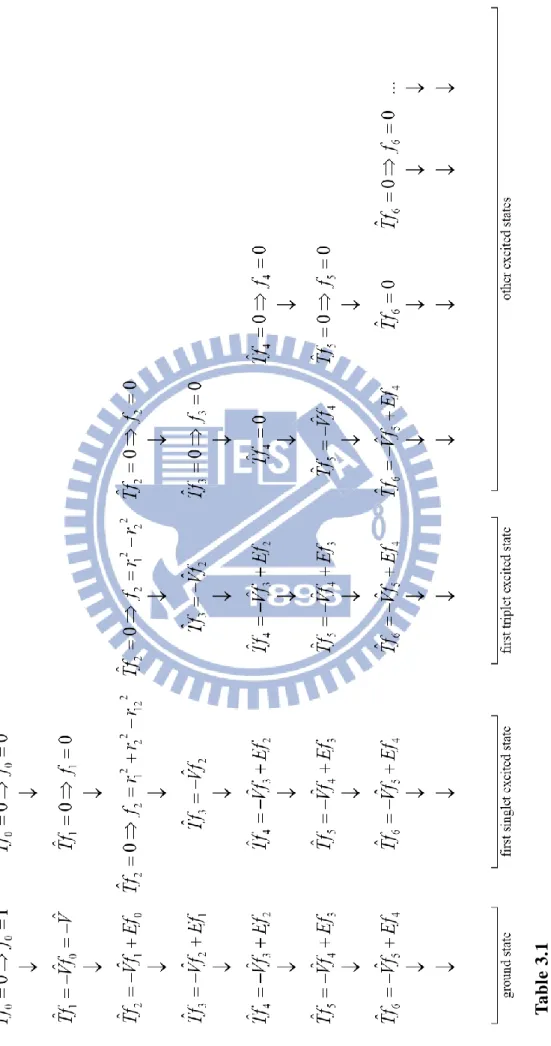
  . If we set  ₀ 0, the wave function represents an excited state. The details of the differences between the wave functions of the ground and excited states are given on the next page (Table 3.1).

T a b le 3 .1 T h e d e ta il o f so lv in g w a v e f u n c ti o n i n t h e g ro u n d s ta te a n d i n e x c it e d s ta te s

Chapter 4

Wave Function of Homogeneity One

After solving the equation with homogeneity zero, the next equation can be

determined by setting  ₀ 1. The equation we discuss becomes

1 0 1 2 12 1 1 1 ˆ ˆ _{( )} T V Z r r r         . (4.1)

To solve this equation, we can expand it into two parts. One part does not contain

12

r , and the other part contains r₁₂1. Eq. (4.1) is then represented as

1,0 1, 1 1,0 1, 1

ˆ( )

T f  f _ g g _ , (4.2)

where f ,_1,0 f_{1, 1} , g1,0 and g1, 1 are defined via

1,0 1,0 1 2 1 1 ˆ _{( )} Tf g Z r r     , (4.3) 1, 1 1, 1 12 1 ˆ Tf g r      . (4.4)

The general solution of ₁ can be written as

1 1,0 1, 1 n 1,n n

f f _ c H

   



 , (4.5)

where H_{m n,} means the n -th homogeneous solution of homogeneity m .

4.1 Solving Terms Independent of

r12

For the terms independent of r , we can change Eq. (4.3) to ratio coordinates ₁₂ (RC) in order to simplify the problem. After changing to ratio coordinates, Eq. (4.3) becomes

1,0 1 1,0 1 ˆ RC_{( , )} RC Z_{(1 )} Tf r g r     . (4.6)

As we know, f_1,0RC has homogeneity one, which means that it can be simplified as

1,0 ( , )1 1 1,0 ( )

RC RC

f r   r f  , (4.7)

and Eq. (4.6) becomes

2 2 2 1 1,0 1,0 1,0 2 1,0 1 1 1 ˆ( ( )) [ ( ) 2 ( ) (1 ) ( )] 2 RC RC d RC d RC T r f f f f r d d                 1 (1 ) Z r    . (4.8)

Eq. (4.8) can be treated as a simple ordinary differential equation

2 2 2 1,0 1,0 2 1,0 1 [ ( ) 2 ( ) (1 ) ( )] (1 ) 0 2 RC d RC d RC f f f Z d d                 . (4.9)

It is easy to find that

2 2 1 2 2 1,0 ( 1 ( ) 3 ) ( 3 ) ( 1) RC C C f   Z                 , and 1,0 1 2 2 1 1 2 1 2 1 1,0 1 ( , ) ( ) ( 1 3 ) ( 3 ) ( 1) RC RC C r C f r r f r   Z r         _{  }   _{ }        , (4.10)

so the final form in the ( , )r r_{1 2} coordinates reads

2 2 1 2 1,0 1 2 1 2 2 1 1 2 1 2 2 1 ( , ) ( ) 3 3 IC r r f r r Z r r C r C r C C r r            . (4.11)

The two terms

2 1 2 r r and 2 2 1 r

r have singularities when r2 0 or r10, respectively. Therefore, C and₁ C should be set to zero to remove the singularities. The ₂ nonsingular solution f_1,0 reads

1,0 (1 2)

f  Z rr . (4.12)

4.2 Expanding Functions in the Power Series of

r₁₂

useful property of the operator ˆT 2 1 2 12 1 1 2 12 2 1 2 12 ˆ_{( ( , )} m₎ ˆ _{( , )} m ˆ _{( , )} m T f r r r  F f r r r F f r r r  , (4.13) where 2 2 1 2 2 1 1 1 2 2 2 1 ( 2) ( 2) ˆ 2 m m F r r r r r r           _    _      , (4.14) 2 2 2 2 1 2 2 1 2 1 1 2 2 ˆ _{( 1)} 2 r r r r m F m m r r r r         _  _      . (4.15)

If m is an odd number, both sides of Eq. (4.13) have only r₁₂ terms in odd powers.

Therefore, we can assume the following ansatz for f_{1, 1}

2 1 1, 1 1, 1,2 1 1 2 12 0 ( , ) k k k f f r r r       



 , (4.16)

since Eq. (4.4) has on the right hand side r₁₂ in an odd power. After substituting Eq. (4.16) into Eq. (4.4), one obtains









2 1 1, 1,2 1 1 2 12 0 12 2 1 2 1 1 1, 1,2 1 12 2 1, 1,2 1 12 2 1 2 1 0 0 12 1 2 1 2 1, 1,1 12 1 1, 1,2 1 2 1, 1,2 3 12 1 2 1 2 3 0 2 2 1 2 1 1 ˆ( ( , ) ) 1 ˆ ˆ ˆ ₁ ˆ ˆ 1 ( 2 k k k k k k k m k m k k k k k k m m k m k k T f r r r r F f r F f r r F f r F f F f r r r r                             _                     









2 2 1 2 1 1, 1,1 12 1 2 2 ) 2 1 r r f r r r r         _{   } _  _{ }        2 2 1, 1,2 1 2 2 0 1 1 1 2 2 2 1 2 3 2 3 ( ) 2 k k k k f r r r r r r                     _{   }    



2 2 2 2 2 1 1 2 2 1 1, 1,2 3 12 1 1 2 2 2 3 (2 3)(2 4) 0 2 k k r r r r k k k f r r r r r     _  _   _   _{  }  _{ }    _{ }         , (4.17)

where Fˆ₁ and Fˆ₂ is defined in Eq. (4.14) and Eq. (4.15).

The first equation we can solve of Eq. (4.17) with r₁₂1 reads 2 2 2 2 1 1 2 2 1 1, 1,1 12 1 1 2 2 1 ( ) 2 1 0 2 r r r r f r r r r r           _{    } _  _{ }        . (4.18)

The solution to Eq. (4.18) is

2 2 2 1 1 2 1, 1,1 1 2 2 2 1 2 ( ) ( , ) r c r r f r r r r       . (4.19)

We easily see that f_{1, 1,1} can have a singularity when r1r2, and f1, 1,1 should

be symmetric with respect to the interchange of r and₁ r . Expanding₂ f_{1, 1,1} as a power series in (r₁r₂) determines value of c which removes the singularity and makes this function be symmetric. After expanding, the function in Eq. (4.19) will become 2 1, 1,1 1 2 1 2 2 (2 1) / 2 3 2 1 ( ) ( ) ... 4 2 8 r c c c f r r r r r           . (4.20)

It is easy to see in Eq. (4.20) that setting 1

2

c  removes the singularity. Therefore,

1, 1,1 f  becomes 2 2 2 1 1 2 1, 1,1 1 2 2 2 1 2 1 ( ) 1 2 ( , ) 2 r r r f r r r r        . (4.21)

The equation corresponding to r₁₂1 can be extracted from Eq. (4.17) as

2 2 1, 1,1 1 2 2 2 1 2 1 1 2 2 1 3 3 ( ) ( , ) 2 r r r r r r f  r r _  _  _  _  _  _{   }  2 2 2 2 1, 1,3 1 2 1, 1,3 1 2 1 2 1 2 1, 1,3 1 2 12 1 1 2 2 ( , ) ( , ) ( ) ( ) 3 3 [ 12 ( , )] 0 2 2 f r r f r r r r r r f r r r r r r r              _    _ . (4.22)

After substituting f_{1, 1,1} from Eq. (4.21) into Eq. (4.22), we can solve for f_{1, 1,3} and get

2 2 1 2 1, 1,3 2 2 2 1 2 ( ) ( ) c r r f r r      . (4.23)

In this case, c must equal to zero to remove the singularity when r₁r₂. Therefore, we easily see that f_{1, 1,3} 0. By this result, we can solve the following equations:

2 2 1, 1,2 1 2 2 1 1 1 1 2 2 2 1 2 3 2 3 ( ) 2 k k k k f r r r r r r                     _{   }    



2 2 2 2 2 1 1 2 2 1 1, 1,2 3 12 1 1 2 2 2 3 (2 3)(2 4) 0 2 k k r r r r k k k f r r r r r     _  _   _   _{  }  _{ }    _{ }         . (4.24) If f_{1, 1,2} _k₁0, Eq. (4.24) becomes 2 2 2 2 1 2 2 1 1, 1,2 3 1 1 1 2 2 2 3 (2 3)(2 4) 0 2 k k r r r r k k k f r r r r     _  _   _   _{  }  _   _{ }      



. (4.25)

The solution of Eq. (4.25) for each k is

2 2 1 2 1, 1,2 3 2 2 2 1 2 ( ) ( ) k k c r r f r r        , (4.26) where kN.

As mentioned above, we know that c must equal to zero to remove the singularity

when r₁r₂ and also makes this function symmetric with respect to the interchange of r and₁ r . So we know ₂ 1, 1,2 1 1 0 2 0 k when k f when k N    _     _  , (4.27) 2 1 1, 1 1, 1,2 1 1 2 12 12 0 1 ( , ) 2 k k k f f r r r r       



  . (4.28)

So we have solved Eq. (4.1) and the solution of Eq. (4.5) has the explicit form.

1 1 2 12 1, 1 ( ) 2 n n n Z r r r c H      



 . (4.29)

For homogeneity one, there are no well-behaving homogeneous solutions which fulfills all of the conditions of a physical wave function. So we finally obtain

1 1 2 12 1 ( ) 2 Z r r r      (4.30)

In this chapter, we introduce two general techniques of solving equations. For the equations without r , we introduce ratio coordinates to simplify the equation ₁₂ into an ODE (Method 1). For equations involving r , we expand our unknown ₁₂ function as a power series in r , so we can solve a family of equations in only two ₁₂ variables (e.g., r and1 r ). After collecting different powers of2 r , the differential 12

equations become first-order partial differential equations (Method 2). Solving this kind of equations is much easier than original differential equations. By using these two techniques, we can gradually tackle the following equations arising in the theory of the wave function of the helium atom.

Chapter 5

Wave Function of Homogeneity Two

5.1 Solving the Equation and Removing Singularities

After solving  ₀ 1 and ₁ (_{1 2}) 1 ₁₂

2

Z r r r

     , we proceed to the next equation Tˆ     ₂ Vˆ ₁ E ₀ to find ₂. 2 2 1 1 2 2 12 1 2 12 1 2 1 2 ( ) 1 1 1 ˆ _{( ) [ ] ( )} 2 2 r r Z Z T r E Z r r r r r r r               . (5.1)

We expand ₂ into three parts

2 2,1 2,0 2, 1 2,1 2,0 2, 1

ˆ _{ˆ( )}

T T f  f  f _ g g g _ , (5.2)

where f ,_2,1 f_2,0 and f_{2, 1} are defined implicitly by

2,1 2,1 12 1 2 1 1 ˆ _{( )} 2 Z Tf g r r r     , (5.3) 2 2 1 2 2,0 2,0 1 2 ( ) 1 ˆ 2 r r Z Tf g E r r       , (5.4) 1 2, 1 2, 1 1 2 12 ˆ _{( )} Tf _ g _   Z r r r  . (5.5)

Since Eq. (5.4) does not contain r , we can use Method 1 to solve this equation. ₁₂ For the remaining two equations, Eq. (5.3) and Eq. (5.5), we use Method 2.

After changing to ratio coordinates, Eq. (5.4) becomes

2 2,0 1 2,0 1 1 1 ˆ _{( , ) ( , ) (2 )} 2 RC RC Tf r  g r  Z  E         (5.6)

zero, and the homogeneity of Tˆ is 2. So we can assume that f_2,0RC( , )r₁  has homogeneity two. Tfˆ_2,0RC( , )r₁  can be written as

2 2 2 2 2,0 1 1 2,0 2 2,0 (1 ) ˆ _{( , )} ˆ_{( ( )) 3 3 ( )} 2 RC RC RC Tf r  T r f     f            _     _     , (5.7)

Therefore, Eq. (5.6) can be rewritten as

2 2 2 2 2,0 2 (1 ) 1 1 3 3 ( ) (2 ) 2 2 RC f Z E              _     _           (5.8)

General solution of this differential equation is given by

2 4 2 2,0 2 1 3 2 2 2 1 1 6 2 3 1 2 ( ) (1 ) 3 6 RC Z E f  C   C                  (5.9)

After changing back to interparticle coordinates, the solution becomes

2 2,0( , )1 2 1 2,0 ( ) 2, IC RC n n n f r r r f  



c H 3 3 2 2 2 2 2 2 1 1 2 1 1 2 2 1 2 2 1 2 2 1 ( 6 ) ( ) ( ) 3 6 3 r r Z E r r C r r C Z r r r r r            2, n n n c H 



 . (5.10)

In Eq. (5.10), we can easily see that C should be set to zero to avoid singularities ₁ when r or₁ r are equal to zero. The value of₂ C must be selected in a way to ₂

make the solution symmetric with respect to the r₁r₂ permutation. After

expanding, Eq. (5.10) becomes

2 2 2 2 2,0 1 2 2 1 2 2 1 2 2, 2 1 ( , ) ( ) 3 3 6 IC n n n Z E f r r C r   C   r Z r r 



c H . (5.11) This equation will be symmetric if

2 2 2 2 1 3 3 6 Z E C   C   , (5.12)