具計算效率且節省記憶體的第三代行動通訊渦輪碼解碼器

全文

(1)國立交通大學電信工程學系碩士班碩士論文具計算效率且節省記憶體的第三代行動通訊(3GPP)渦輪碼解碼器. Calculation Efficient and Memory Saving Turbo Decoder for 3GPP. 研究生：鍾文狀指導教授：紀翔峰博士. 中華民國九十三年八月.

(2) 研究生：鍾文狀. Student: Wen-Choung Chong. 指導教授：紀翔峰博士. Advisor: Dr. Hsiang-Feng Chi 國立交通大學. 電信工程學系碩士班碩士論文 A Thesis Submitted to Deparment of Communication Engineering College of Electrical Engineering and Computer Science National Chiao-Tung University for the Degree of Master in Communication Engineering August 2004 Hsinchu, Taiwan, Republic of China. 中華民國九十三年八月.

(3) 具計算效率且節省記憶體的第三代行動通訊(3GPP)渦輪碼解碼器. 學生：鍾文狀. 指導教授：紀翔峰. 博士. 國立交通大學電信工程學系碩士班. 摘. 要. 目前的無線通訊系統中，資料量的傳輸需求愈來愈大，而在傳輸通道的非理想效應影響下經常使得傳輸資料出現錯誤。為了有效降低錯誤率，第三代行動通訊(3GPP，3GPP2…等)系統均採用了目前更正能力最強的渦輪碼。渦輪碼的硬體實現中最大的難題在於解碼時需要大量的記憶體及大量的運算。一般渦輪碼解碼器中所採用的節省記憶體架構(sliding window)雖可解決記憶體的問題，但同時也會導致更多的運算量。在節省記憶體及運算量的考量下，本論文的目的是以另一種節省記憶體的架構(halfway)實現一個和原始架構比起來可節省記憶體且不增加任何運算量的渦輪碼解碼器。在解碼上，我們採用 Max-Log-MAP algorithm 使得運算複雜度降低。在硬體上，我們使用了只包含一個 Max-Log-MAP 解碼器的硬體架構。. i.

(4) Calculation Efficient and Memory Saving Turbo Decoder for 3GPP. Student: Wen-Choung Chong. Advisor: Dr. Hsiang-Feng Chi. Department of Communication Engineering National Chiao Tung University. ABSTRACT. Turbo codes have become one of the necessary specifications for the state-of-the-art communication systems. The difficulties in implementing turbo decoder are the vast computational complexities and the request for a lot of memories. The most public method for decreasing the need of memories is sliding window method. But using sliding window method will increase the computational complexities. This thesis is purposed to propose a calculation efficient and memory saving turbo decoder. We use another memory saving algorithm – halfway algorithm, in our turbo decoder. This successfully decreases the computational complexities and the need of memory capacity. Besides, we adopt Max-Log-MAP algorithm in our design in order to simplify the hardware.. ii.

(5) 誌. 謝. 短短二年的研究生生涯即將在本論文的完成下告一段落，首先感謝指導教授紀翔峰老師在學業及生涯規劃上的指導，在學業上，老師根據實驗室同學各人的特質，因材施教，讓每位同學自己學得如何自己從無到有的求得知識，在生涯規劃上，老師也盡力地提供自己過去的生活經驗並分析給我們知道。感謝實驗室同學賴昭宏、李昭宏、李佳勳，我們一起在老師的帶領下，把實驗室從無到有地建立起來，而在硬體、軟體實作及論文寫作時，每個人都幫我解決了不少問題，也提供了我很多意見。感謝父母親及哥哥、姊姊讓我在衣食無憂的情況下，得以認真的在實驗室裡做研究，而哥哥有時也會在我的要求下在百忙之中來實驗室教導我們同學如何使用儀器及 FPGA，實在是麻煩他了。最後要感謝的是我的女朋友，楊正豔，從大學以來陪我至今，在六年的求學過程中，她陪在我身邊，無論在學業或生活上遇到困難，她都給予我支持、鼓勵，因此我才能不畏艱難地考上研究所並完成論文寫作。. iii.

(6) Content Content .....................................................................................................................iv List of Figures...........................................................................................................vi List of Tables ......................................................................................................... viii Chapter 1 ...................................................................................................................1 Introduction ...............................................................................................................1 1.1 Digital communication system......................................................................1 1.2 History of channel coding .............................................................................2 1.3 Background of Turbo codes ..........................................................................4 1.4 Motivation and Goal.....................................................................................4 1.5 Thesis Outline...............................................................................................5 Chapter 2 ...................................................................................................................6 Overview of Turbo Code System................................................................................6 2.1 Concatenated Codes .....................................................................................6 2.2 Recursive Systematic Convolutional (RSC) Encoder ....................................7 2.3 Interleavers...................................................................................................9 2.4 Decoders ......................................................................................................9 Chapter 3 .................................................................................................................11 Turbo Decoding .......................................................................................................11 3.1 Decoding Algorithms..................................................................................11 3.1.1 Maximum-a-posteriori (MAP) Algorithm.........................................11 3.1.2 Max-Log-MAP Algorithm................................................................19 3.1.3 Log-MAP Algorithm ........................................................................21 3.1.4 SNR mismatch .................................................................................22 3.1.5 Conclusion.......................................................................................23 3.2 Memory saving methodologies ...................................................................24 3.2.1 Preprocessing over Whole Block Method.........................................25 3.2.2 Sliding Window Method ..................................................................27 3.2.3 Halfway Method ..............................................................................28 3.2.4 Comparisons ....................................................................................30 Chapter 4 .................................................................................................................34 3GPP Turbo Encoder................................................................................................34 4.1 Constituent Encoder ...................................................................................34 4.2 Trellis Termination......................................................................................36 4.3.1 Deciding the size of the rectangular matrix.......................................37 4.3.2 Intra-row and inter row permutations ...............................................39 4.3.3 Output the bits from the rectangular matrix with pruning .................41 iv.

(7) Chapter 5 .................................................................................................................43 Design Considerations..............................................................................................43 5.1 Decoding algorithm selection......................................................................43 5.2 Memory saving method selection................................................................43 5.3 Decision of the block length .......................................................................44 5.4 Analyses of fixed-point representations for calculations ..............................45 5.4.1 Received sequence. yks , ykp , y 'kp ..................................................47. 5.4.2 Branch metrics G k ( s¢, s) ................................................................47 5.4.3 Forward state metrics Ak ( s ) and Backward state metrics Bk ( s ) ..........48 5.4.4 a-priori information LLR L(uk ) , extrinsic information Le (uk ) ...........49 5.4.5 a-posterior LLR L(uk y ) ................................................................51 Chapter 6 .................................................................................................................53 Hardware Architecture .............................................................................................53 6.1 Hardware architecture.................................................................................53 6.1.1 Branch Metrics Unit (BMU).............................................................54 6.1.2 Add-Compare-Select Processor (ACSP)...........................................54 6.1.3 LineCchange unit and BetaChange unit ............................................56 6.1.4 L0,L1 unit ........................................................................................58 6.1.5 Complete turbo decoder architecture ................................................59 6.2 Memory requirements.................................................................................62 6.3 Decoding Process .......................................................................................63 Chapter 7 .................................................................................................................66 Hardware implementation ........................................................................................66 7.1 Design and verify process ...........................................................................66 7.2 Hardware specification ...............................................................................67 7.2.1 Clock cycles for decoding one data frame ........................................67 7.2.2 Hardware interface...........................................................................68 7.3 ASIC performance ......................................................................................69 7.4 FPGA verification.......................................................................................71 Chapter 8 .................................................................................................................73 Conclusion and Future works ...................................................................................73 8.1 Conclusion .................................................................................................73 8.2 Future works...............................................................................................73 References ...............................................................................................................75. v.

(8) List of Figures Figure 1.1: basic elements in digital communication system.......................................1 Figure 2.1: Turbo encoder diagrams of (a) PCCCs (b) SCCCs....................................7 Figure 2.2: (a) RSC encoder with constraint length =3, generator matrix G=[5,7]octal ..8 (b)Non-recursive non-systematic encoder with constraint length =3, generator matrix G=[5,7]octal .................................................................................................................8 Figure 2.3: Conventional turbo decoder’s diagram ...................................................10 Figure 3.1: Evolution of soft-input soft-output (SISO) decoding algorithms .............11 Figure 3.2: possible transitions in K=RSC code........................................................13 Figure 3.3: MAP iterative decoding flow chart .........................................................17 Figure 3.4: Structure of turbo decoder ......................................................................18 Figure 3.5: Various look-up table for Log-MAP .......................................................22 Figure 3.6: Operations on a frame of size N..............................................................25 Figure 3.7: Operations on a frame of size N for preprocessing over whole block ......26 Figure 3.8: Operation flow for sliding window method.............................................28 Figure 3.9: Operations flow for Halfway ..................................................................29 Figure 3.10: Compare the performances of halfway and sliding window ..................33 Figure 4.1: Structure of rate 1/3 Turbo coder ............................................................35 Figure 4.2: Constituent encode of 3GPP turbo encoder and its trellis ........................35 Figure 4.3: Constituent encoder for terminating the trellis ........................................36 Figure 4.4: Interleaving flow chart ...........................................................................42 Figure 5.1: Simulations for various block length ......................................................45 Figure 5.2: Simulations for various precision ...........................................................46 Figure 5.3: Simulations for deciding the integer bits of state metrics ........................49 Figure 5.4: Simulations of various bit length of LLR................................................50 Figure 5.5 performance of our design comparing to floating point ............................52 Figure 6.1: Computation core of the turbo decoder...................................................53 Figure 6.2: Branch metric unit ..................................................................................54 Figure 6.3: ACS processing element .........................................................................55 Figure 6.4: Bundled ACSPEs and the corresponding trellis.......................................55 Figure 6.5: ACS processor and feedback loop...........................................................56 Figure 6.6: (a) trellis diagram for forward state metrics calculations. (b) trellis diagram for backward state metrics calculations. (c) trellis diagram for mapping backward trellis to forward trellis. (d) permutation rules...........................................57 Figure 6.7: (a) BetaChange hardware (b) LineChange hardware...............................58 Figure 6.8: Nesting max operations for L1 hardware ................................................59 Figure 6.9: The block diagram of total turbo decoder hardware ................................60 vi.

(9) Figure 6.10: graphic representation of the halfway SISO algorithm ..........................65 Figure 7.1: develop and design flow .........................................................................67 Figure 7.2: Turbo deocder I/O diagram.....................................................................69 Figure 7.3: ASIC verification flow ...........................................................................70 Figure 7.4: FPGA verification flow ..........................................................................72. vii.

(10) List of Tables Table 3.1: Comparisons of saving memory decoding methods..................................30 Table 4.1: List of prime number p and associated primitive root v ............................38 Table 4.2: Inter-row permutation patterns for Turbo code internal interleaver ...........39 Table 5.1: various memory depths ............................................................................44 Table 5.2: Relationship between L(uk ) and P(uk ) ................................................50 Table 5.3: word length of our design ........................................................................51 Table 6.1: memory capacity......................................................................................62 Table 7.1: decoding clock cycles for different frame size..........................................68 Table 7.2: I/O ports definition ..................................................................................69 Table 7.3: ASIC simulation results ...........................................................................70 Table 7.4: required clock rate for decoding different frame size and iteration............71. viii.

(11) _________________________________________ Chapter 1 Introduction _________________________________________ In this chapter, we will introduce the basic elements of the digital communication system and the concept of channel coding in the beginning. Then the motivation and the objective of this thesis are presented. Finally we will introduce the organization of this thesis.. 1.1 Digital communication system The basic elements of a digital communication system are shown in Figure 1.1.. Figure 1.1: basic elements in digital communication system. The messages from the source are converted into a sequence of binary digits by source encoder. The process of efficiently converting the output of the source into a sequence of binary digits is called source encoding. Alternatively speaking, the source encoder compresses the data from source and result in little or no redundancy in the 1.

(12) binary representations of the data. Then the sequence of binary digits from the source encoder is passed to the channel encoder. On the contrary, the channel encoder is to introduce some controlled redundant information in the binary information sequence. These added redundancies can help the receiver to overcome the noise and interference encountered in the transmission of the signal through the channel. In effect, redundancy in the information sequence aids the receiver in decoding the information sequence correctly. The main purpose of the modulator is to map the binary information sequence into signal waveforms. We can choose modulator according to different applications and different channels. Usually we use the additive white Gaussian noise channel to simulate the channel block because it can provide precise analyses. At the receiving end of a digital communication system, the successive three blocks are used to recover the original signals from the noisy receiving sequence. The demodulator processes the noisy waveforms and reduces them to a sequence of numbers that represent estimates of the transmitted symbols. The channel decoder will use these numbers to reconstruct the original information sequence from knowledge of the channel encoder. The source decoder uncompresses the sequence from knowledge of the source encoder and attempts to reconstruct the original signals. The subject of the channel encoder and channel decoder is called channel codes or error control codes. In this thesis, we focus on this subject, especially the hardware implementation of the channel decoder.. 1.2 History of channel coding The concept of channel coding came from the paper [1] which was published by Claude Shannon in 1948. Shannon’s primary result in this area is called the channel. 2.

(13) capacity theorem or noisy channel coding theorem. This theorem states that there exist error control codes such that information can be transmitted across the channel at rates less than the channel capacity with arbitrarily low bit error rate. Unfortunately, Shannon did not show how to construct the codes which can achieve the channel capacity. Two categories of channel codes, block codes and convolutional codes, were developed and widely used in practical systems. The first error correcting code was Hamming code [2], which can correct only one error. During the years from 1957 to1959, cyclic codes [3-5] were published in some reports by E. Prange. Cyclic codes led to the development of BCH codes and Reed-Solomon codes a few years later. In 1959 and 1960 [6-8], Bose and Ray-Chaudhuri and Hocquenghem discover the multiple error correcting codes which are later named as Bose-Chaudhuri-Hocquenghem (BCH) codes. Reed-Solomon codes were discovered in 1960 by Reed and Solomon [9] and they were closely related to BCH codes. In 1955, the first convolutional forward error correction codes were discovered by Elias [10]. In 1961, Wozencraft and Reiffen proposed the sequential decoding algorithm [11, 12] and this decoding algorithm is fast but sub-optimum. In 1967, Viterbi proposed an optimum decoding algorithm [13] which was recognized by Forney [14] as maximum likelihood decoding algorithm in 1973. In 1987, Ungerboeck proposed trellis coded modulation (TCM) [15, 16] which integrates forward error correcting codes and modulation. TCM can achieve significant coding gains over power and band-limited transmission media. In 1993, turbo codes [17] were invented by C. Berrou, A. Glavieux and P. Thitimajshima. Turbo codes were a historic breakthrough because they help the communication systems achieve Shannon limit closer than other codes.. 3.

(14) 1.3 Background of Turbo codes Since turbo codes were proposed by C. Berrou, A. Glavieux and P. Thitimajshima in 1993 [17], they have been widely studied and discussed. Till now they are known as the best forward error correcting codes. Due to turbo codes’ outstanding error correcting performance and their ability to achieve the Shannon capacity limit by 0.7 dB [17], there are many researches on the realizations of turbo codes. Turbo codes outperformed all other known coding schemes. Recently turbo codes have been adopted in several standardized communication systems, such as the third-generation (3G) mobile communication standards: i.e. W-CDMA (Wideband Code Division Multiple Access) in the 3rd Generation Partnership Project (3GPP), cdma2000 in the 3rd Generation Partnership Project 2 (3GPP2), and TD-SCDMA (proposed by China and Japan).. 1.4 Motivation and Goal Turbo codes have become one of the necessary specifications for the state-of-the-art communication systems. How to efficiently realize the turbo decoder in the integrated circuit always cause much research attention. The difficulties in designing turbo decoders come from the high computational complexity. The challenging tasks are how to reduce the hardware cost and power consumption, the word-length determination in the fixed-point arithmetic, and cost-effective memory allocation/partition. In this thesis, we aim at implementing the turbo decoder of 3GPP/W-CDMA on field-programmable gate arrays (FPGAs) with memory saving methods. We will use Max-Log-MAP algorithm to solve the difficulty of the computational complexity. The ultimate goal is to propose low complexity, calculation efficient and memory-saving architecture. 4.

(15) 1.5 Thesis Outline This thesis is organized into eight chapters and described as follow: In chapter 2, we would have an overview of entire turbo code system. In chapter 3, we introduce several decoding algorithms, discuss, and compare four decoding methods, including three memory saving schemes. In chapter 4, the 3GPP turbo encoder and interleaver are described. The hardware design considerations are discussed in chapter 5. In chapter 6, we describe the hardware architecture in detail. The ASIC and FPGA implementation and verification processes are presented in chapter 7. The conclusion and the future works are presented in Chapter 8.. 5.

(16) _____________________________________________________________________. Chapter 2 Overview of Turbo Code System _____________________________________________________________________. Turbo codes use concatenated schemes with the interleavers/de-interleavers placed between the constituent encoders/decoders. The standard turbo encoder structure uses the recursive systematic convolutional codes and parallel concatenated convolutional codes. In order to achieve good BER performance, we need the decoding algorithms which can accept soft input and produce soft outputs and can work iteratively.. 2.1 Concatenated Codes Turbo codes are usually composed of several concatenated convolutional codes. There are two kinds of concatenated convolutional codes, one is parallel concatenated convolutional codes (PCCCs) and the other is serial concatenated convolutional codes (SCCCs). PCCCs are often constituted by two or more recursive systematic convolutional (RSC) encoders joined in parallel by one or more pseudo-random interleavers, furthermore, the encoders encode the same information bits besides the information bits are scrambled by the interleaver. SCCCs also use the constituent convolutional encoder and the interleavers as PCCCs but differ from their connection method. The encoders used in SCCCs are connected serially and inserted by the pseudo-random interleaver. Figure 2.1 shows the encoder diagram of PCCCs and SCCCs.. 6.

(17) Figure 2.1: Turbo encoder diagrams of (a) PCCCs (b) SCCCs. The advantage of SCCCs is that: for a fixed frame size N, the slope of BER curve is inversely related to N2 or N3 but BER curve for PCCCs is only inversely related to N. Beside, SCCCs do not suffer from error floor but PCCCs do. The problem of error floor is caused by the poor interleaver design and truncation in the decoding procedure. But it was shown that both SCCCs and PCCCs could be designed without suffering from error floor no matter what BER requirement is [18]. Although SCCCs have the merits mentioned above, we often choose PCCCs in turbo code due to PCCCs’ less computational complexity given the same constituent encoders and their better BER performance at low SNRs. Throughout the rest of this thesis, “turbo code” is referred to use PCCCs.. 2.2 Recursive Systematic Convolutional (RSC) Encoder Turbo codes use two or more RSC encoders as their component encoder. Although the encoders need not to be the same, we often use identical encoders in practice due to the low complexity of decoding. The term “recursive” means the. 7.

(18) encoder has a feedback loop; therefore, the output of this encoder is affected by the preceding output bit. And the term “systematic” means the encoder has one of its outputs identical to its input bit. Figure 2.2 shows the conventional convolutional encoder.. Figure 2.2: (a) RSC encoder with constraint length =3, generator matrix G=[5,7]octal (b)Non-recursive non-systematic encoder with constraint length =3, generator matrix G=[5,7]octal. It can be proved that the recursive systematic convolutional code is code-equivalent to the non-systematic non-recursive convolutional code [19]. That is the sets of the codewords that they define are the same and for any codeword of the recursive systematic convolutional encoder, we can find the input stream for the non-systematic non-recursive convolutional code such that it produces the same codeword, vice versa. Although their codewords are identical, they behave differently. It is also shown that the RSC encoder tends to produce codewords with more weights than the code-equivalent non-recursive encoder [20]. This behavior causes the RSC encoder produce fewer codewords with lower weights and makes the error correcting performance better. This is the main reason to use the RSC encoders as turbo codes’ constituent encoders. Additionally, when we use the RSC encoder as constituent encoder, we only need to transmit the systematic output bits from the first one encoder. 8.

(19) because their systematic bits are alike except the order. Then the code rate of the encoder increases, bandwidth efficiency improves without degrading the performance since we still transmit all the information produced by the encoder.. 2.3 Interleavers The interleavers placed between the encoders are going to make the code more random in order to improve the burst error correction capability and they play a key rule in turbo code. What affect the interleaver are how random the interleaver is and how big the size of the interleaver is. As the size of the interleaver grows, the performance of the turbo code usually becomes better. But there is a tradeoff between the decoding latency and the BER performance. When the interleaver is more likely random, the performance of the turbo code also becomes better due to this kind of interleaver can make the correlation of the information bits decrease more. There are several kinds of interleavers, e.g. column-row interleaver, helical interleaver, odd-even interleaver, simile interleaver, frame interleaver, pseudo-random interleaver, S-type interleaver…etc. As long as we use the interleaver we proposed, the performance of the turbo code will suffer and we need to use different kind of interleaver according to the system requirement.. 2.4 Decoders Although the constituent encoders for turbo code belong to convolutional encoders, the decoding scheme for turbo codes is different from the pure convolutional decoding scheme. As mentioned above, turbo codes use the parallel concatenated encoding scheme. The turbo decoder would be constructed on the serial concatenated scheme because the performance of serial concatenated decoding 9.

(20) scheme is better than that of parallel concatenated decoding scheme. The reason is the serial concatenated decoder will provide some extra information (or we call extrinsic information in turbo codes) to another decoder as its a-prior information. In turn, the latter decoder will also provide extra information to the former one. Contrarily the parallel concatenated decoders decode the information independently. Figure 2.3 shows the conventional turbo decoder’s diagram.. Figure 2.3: Conventional turbo decoder’s diagram. Because each component decoder must provide the a-prior information to the other, they must have soft outputs. Since they have the soft inputs, we call them soft-input soft-output (SISO) decoders.. 10.

(21) ______________________________________________. Chapter 3 Turbo Decoding ______________________________________________ Nowadays we have two categories of algorithms to decode turbo codes, one originates from Maximum a posteriori (MAP) algorithm [21] proposed by Bahl et al. and another is Soft-Output Viterbi algorithm (SOVA) [22] proposed by Hagenauer and Hoeher. Their evolutional histories are shown in Figure 3.1.. Figure 3.1: Evolution of soft-input soft-output (SISO) decoding algorithms. 3.1 Decoding Algorithms 3.1.1 Maximum-a-posteriori (MAP) Algorithm The Log Likelyhood Ratios (LLRs) L( uk ) of a data bit uk is defined to be the log of the ratio of the probabilities of the bit taking its two possible values: 11.

(22) æ P(uk = +1) ö L(uk ) @ ln ç ÷ è P(uk = -1) ø. (1). where P(uk = ±1) is the probability of the data bit uk equals to ±1 . After encoding the data bit uk and transmitting the encoding bits through the channel and the matched filter, we received the sequence y . Therefore we get the conditional LLR defined as: æ P(uk = +1 | y ) ö L(uk | y ) @ ln ç ç P(u = -1 | y ) ÷÷ k è ø. (2). These conditional probabilities P(uk = ±1| y ) are the a-posteriori probabilities of the decoded bit uk . The goal of the MAP algorithm is to estimate the decoded bit sequence and provide the probabilities of the correctness of every decoded bit given the received sequence y and it aims at minimizing the decoded bit error rate (BER). This means the MAP algorithm is correspondent with finding the a-posteriori LLR L(uk | y ) . By using Baye’s rule and its derivation, P ( a Ù b ) = P ( a b ) × P ( b). (3). P({a Ù b} c ) º P( a {b Ù c}) × P(b c). (4). the a-posteriori LLR L(uk | y ) can be rewritten as: æ P(uk = +1 Ù y ) ö L(uk | y ) = ln ç ç P(uk = -1 Ù y ) ÷÷ è ø Figure 3.2 is the possible trellis for K=3 RSC code.. 12. (5).

(23) Figure 3.2: possible transitions in K=RSC code If the previous state S k -1 = s¢ and the present state S k = s are known then the input bit uk will be known. The transitions which occur when uk = +1 and those which occur when uk = -1 are mutual exclusive so that the probability that any one of them occurs is equal to the sum of their individual probabilities. Equation (5) can be written as: æ å P( Sk -1 = s ¢ Ù Sk = s Ù y ) ö ç ( s ¢ , s )Þ ÷ uk =+1 ç ÷ L(uk | y ) @ ln ç å P( Sk -1 = s ¢ Ù Sk = s Ù y ) ÷ ç ( s ¢ , s )Þ ÷ è uk =-1 ø. (6). Assume the channel is memoryless and using the Bayes’ rule, we can write the individual. probabilities. P( S k -1 = s ¢ Ù S k = s Ù y ). from. the. numerator. and. denominator as: P( s¢ Ù s Ù y ) = P( s¢ Ù s Ù y j <k Ù yk Ù y j >k ) = P( s¢ Ù s Ù y j <k Ù yk ) × P( y j >k s ¢ Ù s Ù y j < k Ù yk ) = P( s¢ Ù s Ù y j <k Ù yk ) × P( y j >k s ) = P( s¢ Ù y j < k ) × P ({ yk Ù s} {s ¢ Ù y j < k }) × P( y j > k s ) = P( s¢ Ù y j < k ) × P ({ yk Ù s} s ¢) × P ( y j >k s ) = a k -1 (s ¢) × g k ( s¢, s ) × b k ( s ) 13. (7).

(24) where P( s¢ Ù s Ù y ) represents P( S k -1 = s ¢ Ù S k = s Ù y ) for simplicity, and a k -1 (s ¢) ,. b k ( s ) , g k ( s¢, s ) are shown below: a k -1 ( s¢) = P( Sk -1 = s¢ Ù y j<k ). (8). b k ( s ) = P ( y j >k Sk = s ). (9). g k ( s¢, s ) = P ({ yk Ù Sk = s} Sk -1 = s¢) .. (10). Using Bayes’ rule and the assumption that channel is memoryless, a k ( s ) can be written as:. a k ( s ) = P( Sk = s Ù y j < k +1 ) = P( s Ù y j <k Ù yk ) = å P( s¢ Ù s Ù y j < k Ù yk ) all s ¢. = å P({s Ù yk } {s¢ Ù y j <k }) × P(s ¢ Ù y j < k ). (11). all s ¢. = å P({s Ù yk } s¢) × P( s¢ Ù y j <k ) all s ¢. = å g k ( s¢, s ) × a (s ¢) all s ¢. Assuming the trellis has the initial state S 0 = 0 , the initial conditions for a k ( s ) are:. a0 ( S0 = 0) = 1 a0 ( S0 = s ) = 0 for all s ¹ 0. (12). Similar to the derivation of a k ( s ) , b k -1 ( s ¢) can also be written as:. b k -1 ( s¢) = å b k ( s ) × g k ( s¢, s ). (13). all s. If the trellis is terminated in the all-zero state, the initial conditions for b k ( s ) are:. b N (0) = 1 b N ( s) = 0 s ¹ 0. (14). If the trellis is not terminated, then the initial conditions for b k ( s ) are:. b N ( s ) = 1 for all s. (15). where N is the number of the stages in the trellis. Thus, once the g k ( s¢, s ) values are known, a k ( s ) and b k -1 ( s ¢) values can be calculated recursively. 14.

(25) Using the derivation from Bayes’ rule, g k ( s¢, s ) can be written as:. g k ( s¢, s ) = P({ yk Ù s} s¢) = P( yk {s¢ Ù s}) × P(s s ¢) = P( yk {s¢ Ù s}) × P(uk ). (16). = P( yk xk ) × P(uk ) where uk is the input bit which would cause the transition from state S k -1 = s¢ to state S k = s and xk is the corresponding transmitted codeword. P(uk ) is the a-prior probability of this input bit uk . Assuming the channel is Gaussian and using BPSK modulation, g k ( s¢, s ) can be written as:. g k ( s¢, s ) = P(uk ) × P( yk {s¢ Ù s}) = C × e ( uk ×L ( uk ) / 2) × exp(. n Eb 2 a xkl ykl ) × × å 2s 2 l =1. æL = C × e ( uk ×L ( uk ) / 2) × exp ç c è2. n. åx l =1. kl. (17). ö ykl ÷ ø. where C is the term does not depend on the sign of the bit uk and the transmitted codeword xk , n is the number of the bits in codeword xk . Lc is called channel reliability value and defined as: Lc =. Eb × 4a 2s 2. (18). where Eb is the transmitted energy per bit, s 2 is the noise variance and a is the fading amplitude( a = 1 for non-fading AWGN channels). Finally the a-posteriori LLR L(uk y ) in equation (6) can be rewritten as: æ å a k -1 × g k (s ¢, s ) × b k ( s ) ö ç ( s ¢ , s )Þ ÷ uk =+1 ç ÷ L(uk y ) = ln ç å a k -1 × g k (s ¢, s ) × b k ( s ) ÷ çç ( s¢, s )Þ ÷÷ è uk =-1 ø This conditional LLR L(uk y ) is what MAP algorithm wants to get. 15. (19).

(26) Because the turbo codes use RSC, we can separate g k ( s¢, s ) into two parts. One has relationship with the systematic bit and the other does not. When we assume the systematic bit is the first bit of n transmitted bits, xk1 = uk , we get: æL n ö g k ( s¢, s ) = C × e(uk × L (uk ) / 2) × exp ç c å xkl ykl ÷ è 2 l =1 ø æL æL ö = C × e(uk × L (uk ) / 2) × exp ç c uk yks ÷ × exp ç c è 2 ø è 2. n. åx l =2. kl. ö ykl ÷ ø. (20). æL ö = C × e(uk × L (uk ) / 2) × exp ç c uk yks ÷ × c k ( s¢, s ) è 2 ø where c k ( s¢, s ) is the part uncorrelated with the systematic bit and it is shown below: æL c k ( s¢, s ) = exp ç c è 2. n. åx l =2. kl. ö ykl ÷ ø. (21). Then we can separate the a-posteriori LLR L(uk y ) into three parts and rewrite it as follows: æ å a k -1 × e( + L (uk ) / 2) × e( + Lc yks / 2 ) × c k (s ¢, s ) × b k ( s ) ö ç ( s ¢, s )Þ ÷ uk =+1 ç ÷ L(uk y ) = ln ç ( - Lc yks ) ( - L ( uk ) / 2) a k -1 × e ×e × c k ( s¢, s ) × b k (s ) ÷ ç ( så ÷ s )Þ ç u ¢,=÷ 1 è k ø æ å a k -1 × c k (s ¢, s ) × b k ( s ) ö ç ( s ¢ , s )Þ ÷ uk =+1 ç ÷ = L(uk ) + Lc yks + ln ç å a k -1 × c k (s ¢, s ) × b k ( s ) ÷ çç ( s¢, s )Þ ÷÷ è uk =-1 ø = L(uk ) + Lc yks + Le (uk ). (22). where: æ å a k -1 × c k (s ¢, s ) × b k ( s ) ö ç ( s ¢ , s )Þ ÷ uk =+1 ç ÷ Le (uk ) = ln ç å a k -1 × c k (s ¢, s ) × b k ( s ) ÷ çç ( s ¢, s )Þ ÷÷ è uk =-1 ø. (23). The first term L(uk ) is the a-prior LLR which can be derived from P(uk ) and. 16.

(27) it is usually unknown at the decoder. Because we usually assume P(uk = ±1) = 0.5 at first time, the initial conditions of L(uk ) are all zero in the logarithm domain. But when we use iterative turbo decoder, each component decoder can provide the other one with the a-prior LLRs. The second term Lc yks stands for the soft output of the channel when the input systematic bit uk transmitted through the channel and received as yks . Because the channel reliability value Lc is directly relative to the channel SNR, the received systematic bit yks will have a large impact on the a-posteriori LLR L(uk y ) if the channel SNR is high and vice versa. The third term Le (uk ) is referred to as the extrinsic LLR for the bit uk because it uses the values of the branch transition probabilities g k ( s¢, s ) for all the branches except for the k-th branch. Then it will be sent to the next decoder as the a-prior information. The flowchart of all the operations involved in MAP algorithm and iterative decoding process is shown in Figure 3.3. L(uk ) = 0. A-priori info.. Channel Values. Lc y kl. L ( uk ). Evaluate. g k ( s¢, s). Evaluate. a k -1 ( s ) Lc yks. Calculate LLR. L( uk | y ). Evaluate. b k ( s). Calculate Le. Le (uk | y ). to next decoder. Figure 3.3: MAP iterative decoding flow chart 17.

(28) The structure of the turbo decoder is shown in Figure 3.4. It is constituted by two component decoders, one interleaver and one deinterleaver and the decoders will work iteratively. Each component decoder has three inputs: 1. the systematic information 2. The parity information associated the component encoder and 3. The information provided by the other component decoder which was referred to as a-prior information. Lc yks. L( uk | y ). Le12 (uk ). Lc ykl. L (uk ). Lc yks. L( uk | y ). Le21 (uk ). Lc ykl L ( uk ). Figure 3.4: Structure of turbo decoder We describe the iterative decoding process as follow: Firstly the component decoder 1 takes the systematic bits in natural order and the parity bits transmitted by the encoder 1 as its input signals but take the a-prior information, which should get from component decoder 2, as 0 since the component decoder 2 does not take action. After finish the decoding of the decoder 1, the decoding result or the a-prior information should be transferred to the decoder 2 in interleaving order. Secondly the decoder 2 takes the parity bits transmitted by the encoder 2, the systematic bits in interleaving order and the a-prior information provided by the decoder 1 in interleaving order as its input signals. When the decoder 2 finishes its 18.

(29) decoding process, it also produces the a-prior information for the decoder 1 but in the interleaving order, then transferring the a-prior information with the aid of the de-interleaver to the decoder 1. The first iteration completes after these steps and we can repeat again besides the decoder 1 has the a-prior information this time. Usually after 5 to 10 times iterations, the decoder will output the decoding results. Because the iterative decoding process is similar to the cyclic feedback mechanism of the turbo engine, we name the code “turbo code”.. 3.1.2 Max-Log-MAP Algorithm The Max-Log-MAP algorithm simplifies the calculations of a k ( s ) , b k ( s ) and. g k ( s¢, s ) which are needed by MAP algorithm by transferring these calculations into the log arithmetic domain and using the Jacobian logarithm approximation loosely: æ ö ln ç å e xi ÷ » max( xi ) i è i ø. (24). where max( xi ) is the maximum value of xi . i. By defining Ak ( s ) , Bk ( s ) and G k ( s¢, s ) as the logarithm of a k ( s ) , b k ( s ) and g k ( s¢, s ) , we can rewrite the equations as follows: Ak ( s ) @ ln (ak ( s ) ) æ ö = ln ç å a k -1 ( s¢)g k ( s¢, s ) ÷ è all s¢ ø æ ö = ln ç å exp [ Ak -1 ( s¢) + G k ( s¢, s )] ÷ è all s¢ ø » max ( Ak -1 ( s¢) + G k ( s¢, s ) ). (25). s¢. Bk -1 ( s¢) @ ln ( b k -1 ( s¢) ). » max ( Bk (s ) + G k (s ¢, s ) ). (26). s. Equation (25) is calculated in a forward recursive manner and equation (26) is. 19.

(30) Ak ( s ) = max ( Ak ( s ') + G k ( s ', s ) ) calculated in a backward recursive manner but they s'. are both equivalent to the recursion used in the Viterbi algorithm – for the merging paths the survivor is found by using additions and comparison. Then the new branch metric G k ( s¢, s ) can be written as: G k ( s¢, s ) @ ln ( g k ( s¢, s ) ) n æ é E ùö = ln ç C × e(uk ×L (uk ) / 2) exp ê b 2 2a å ykl xkl ú ÷ ë 2s ûø l =1 è æ éL n ùö = ln ç C × e(uk ×L (uk ) / 2) exp ê c å ykl xkl ú ÷ ë 2 l =1 ûø è. L 1 = Cˆ + uk × L(uk ) + c 2 2. (27). n. åy l =1. x. kl kl. where Cˆ = ln(C ) does not have any relationship with the data bit, uk ,or the codeword, xk , and so can be considered a constant and ignored. From equation (19), the a-posteriori LLRs L(uk y ) for Max-Log-MAP algorithm can be calculated as: æ å a k -1 ( s¢) × g k ( s¢, s ) × b k ( s ) ö ç ( s¢, s )Þ ÷ u =+1 ÷ L(uk y ) = ln ç k ç å a k -1 ( s¢) × g k ( s¢, s ) × b k ( s ) ÷ ç ( s¢, s )Þ ÷ è uk =-1 ø æ å exp ( Ak -1 ( s ¢) + G k ( s¢, s ) + Bk ( s ) ) ö ç ( s¢, s )Þ ÷ u =+1 ÷ = ln ç k ç å exp ( Ak -1 ( s ¢) + G k ( s¢, s ) + Bk ( s ) ) ÷ ç ( s¢, s )Þ ÷ è uk =-1 ø » max ( Ak -1 ( s¢) + G k ( s¢, s ) + Bk ( s ) ). (28). ( s¢, s )Þ uk = +1. - max ( Ak -1 ( s¢) + G k ( s¢, s ) + Bk ( s ) ) ( s¢, s )Þ uk =-1. The transitions from the trellis stage S k -1 to the stage S k are grouped into two groups. One contains those might happen if uk = +1 and the other contains those. 20.

(31) might happen if uk = -1 . In each group, we only want the maximum value of. ( Ak -1 ( s¢) + Gk ( s¢, s) + Bk (s ) ). and the a-posteriori LLRs L(uk y ) can be calculated as. their difference.. 3.1.3 Log-MAP Algorithm It was found by Robertson et al. [23] Max-Log-MAP algorithm would result in worse performance than MAP algorithm when used iterative decoding due to the rough approximation. But the approximation can be made exact by using the Jacobian logarithm:. (. - x -x ln( e x1 + e x2 ) = max( x1, x2 ) + ln 1 + e 1 2. = max( x1, x2 ) + f c ( x1 - x2 ). ) (29). = g ( x1 , x2 ) where f c (s ) stands for a correction term and s equals to the magnitude of the difference between x1 and x2 . f c (s ) need not be computed for every value of s , but instead can be stored in a look-up table. There are several ways to implement the look-up table and make the algorithm have other names such as constant-log-MAP, linear-log-MAP algorithms.. f c (s ). s 21.

(32) Figure 3.5: Various look-up table for Log-MAP For binary trellises Ak ( s ) and Bk -1 ( s¢) can be written as: Ak ( s ) @ ln (a k ( s ) ) æ ö = ln ç å exp [ Ak -1 ( s ¢) + G k (s ¢, s )] ÷ è all s¢ ø » max ( ( Ak -1 (s ¢) + G k (s ¢, s ) ) , ( Ak -1 (s ¢¢) + G k (s ¢¢, s ) ) ) + fc. ( (A. k -1. ( s¢) + G k ( s¢, s ) ) - ( Ak -1 ( s¢¢) + G k ( s¢¢, s ) ). (30). ). Bk -1 ( s¢) @ ln ( b k -1 ( s¢) ). » max ( ( Bk (s ) + G k (s ¢, s ) ) , ( Bk (s ¢¢) + G k ( s¢, s ¢¢) ) ) + fc. (31). ( ( B (s ) + G (s¢, s) ) - ( B (s¢¢) + G (s¢, s¢¢) ) ) k. k. k. k. Because there will be 2 × 2 K -1 transitions at each stage of the trellis for binary trellis, there will be 2 K -1 transitions in each of the maximizations in equation (30) (31), where K is the constraint length of the convolutional code. If we want to apply the Jacobian logarithm to it, we need to nest the g ( x1 , x2 ) operations. Then we should use the nesting equation shown below:. (. ) ). æ I ö ln ç å e xi ÷ = g x I , g x I -1 ,L, g ( x3 , g ( x2 , x1 ) ) L è i =1 ø. (. (32). 3.1.4 SNR mismatch According to [24] [25], the BER performance of the Log-MAP algorithm would decrease if the channel’s SNR ratio estimation is not estimated correctly. As the frame size of Turbo code increases, the effect on BER performance would become more severe. Contrarily the BER performance of Max-Log-MAP will not be affected by the mismatched SNR. The reason for BER performance affected by SNR mismatch is the non-linear character of Log-MAP algorithm. The difference between Max-Log-MAP algorithm 22.

(33) and Log-MAP algorithm is the correction term on the right hand side in equation (29). The correction term results in non-linear character of Log-MAP algorithm. When we calculate the branch metrics, state metrics, a-posterior LLR and extrinsic information iteratively, their values will be affected by the non-linear term. Since the approximation used by Max-Log-MAP algorithm is linear, the branch metrics, state metrics, a-posterior LLR and extrinsic information all will be scaled by Lc simultaneously. Therefore, we can let Lc equal to one in the calculations.. 3.1.5 Conclusion As mentioned, there are two kinds of SISO decoding algorithms could be adopted in the turbo decoder. One is the family of MAP algorithms and the other is SOVA. Although [23] claims that the SOVA has only half the complexity of the Max-Log-MAP, there are other researches [26] find SOVA is more complex than Max-Log-MAP unless the decoder using SOVA is designed carefully. No matter how the decoder using SOVA is implemented, the BER performance is worse than or equal to (at most) the performance of Max-Log-MAP. Therefore we do not discuss about SOVA in this thesis. The original MAP algorithm does not suit to be implemented on the hardware due to it needs many multiplications and exponential calculations. Therefore, the most popular Turbo decoding algorithms derived from MAP algorithm and have been adopted in the hardware implementations are Log-MAP and Max-Log-MAP algorithms. As we described, Max-Log-MAP algorithm is a simplified version of Log-MAP algorithm and the former BER performance is slight worse than the latter one. But according to the analyses from [26], the computational complexity of Log-MAP algorithm is 2 to 3 times as complex as Max-Log-MAP. According to section 3.1.4, Log-MAP algorithm suffers from SNR mismatch 23.

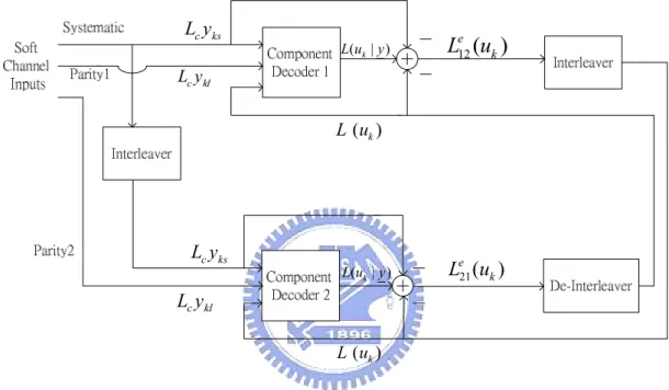
(34) problem but Max-Log-MAP algorithm does not. Even if the channel SNR could be estimated correctly real time, Log-MAP algorithm still needs several lookup tables in the hardware implementation but Max-Log-MAP does not. In fact, the channel varies at any time and on-line SNR estimation is impracticable to some degree. Therefore we implement Max-Log-MAP algorithm on our hardware.. 3.2 Memory saving methodologies In turbo decoding, the memory part always plays an important rule because it occupies most of the area of the decoder. In this chapter, we will introduce the original decoder structure and there kinds of saving memory decoding method, including preprocessing over whole block method, preprocessing over window method and halfway method. Finally we will compare these methods in memory capacity aspect. When we say memory capacity in this section, we mean those used to store the state metrics. From equation (28) the a-posteriori LLRs L(uk y ) are calculated as: L (uk y ) = max ( Ak -1 ( s ¢) + G k ( s ¢, s ) + Bk ( s ) ) - max ( Ak -1 ( s ¢) + G k ( s ¢, s ) + Bk ( s ) ) ( s¢, s ) Þ uk =+1. ( s¢, s ) Þ uk =-1. That means we must have the values of Ak -1 ( s¢) , G k ( s¢, s ) and Bk ( s ) at first. As we know, Ak -1 ( s¢) is calculated in forward recursive manner and Bk ( s ) is calculated in backward recursive manner. Assume the inputs to the encoders are binary, the component encoder has constraint length K and the data need to be decoded have a frame length N. We do the backward recursion first due to be capable of making decisions in the usual order of the data. In order to make decisions over the whole frame, the state metrics calculated during the first processing (backward) must be memorized. Then the required memory. 24.

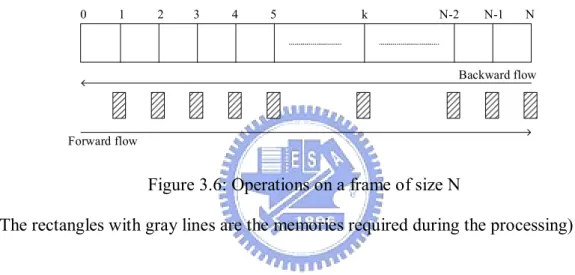
(35) size for a received frame length N is M r = N × 2 K -1 × q , where q is the number of quantization binary digits. The operations flow and the memory required are shown in Figure 3.6. We take the specification from 3GPP turbo code for example, the maximum frame length (Nmax) is 5114 and the constraint length (K) is 4 so that if we set the number of quantization bits ( q ) equal to 10, we will need about 410 Kbits. In most case, reducing the size of the memory is necessary.. 0. 1. 2. 3. 4. 5. k. N-2. N-1. N. Backward flow. Forward flow. Figure 3.6: Operations on a frame of size N (The rectangles with gray lines are the memories required during the processing). 3.2.1 Preprocessing over Whole Block Method The first method for reducing the memory size uses the concept of initialization. The initialization process precedes the first processing in the same order (backward). Choose a number L as the length of a block and calculate the number p by êN ú p = ê ú , then the forward flows and backward flows are subdivided into p ëLû sub-process. The operations flow and the memory required are shown in Figure 3.7.. 25.

(36) ( p - 1) × L. Figure 3.7: Operations on a frame of size N for preprocessing over whole block (The rectangles with gray lines are the memories required during the processing of making decision and the black rectangles represent the memories for initialization). In the beginning, we perform the backward calculations and store the backward state metrics in the memories (which are indicated as black rectangles in Figure 3.7 periodically (period=L). The stored values will serve as initialization metrics for the backward sub-processes. So the backward flow is carried out on successive windows of size L, where the starting state metrics are known. The capacity of the memory for initialization is M ri = ( p - 1) × 2 K -1 × q . The capacity of the memory for making decisions is M rd = L × 2 K -1 × q for using only one ACS processor. If using two ACS processors, it can be shown that the required memory size can decrease as M rd = ( L - 1) × 2 K -1 × q . So the overall required memories are. Mtotal = ( L + p -1) × 2K -1 × q. for. using. one. ACS. processor. and. Mtotal = ( L + p - 2) × 2K -1 × q for using two ACS processors. In general, we choose p = L » éê N ùú because this choice can offer the minimal memory capacity.. 26.

(37) We take the 3GPP Turbo encoder for example again and let q = 10 , we get: p = L » éê N ùú = éê 5114 ùú = 72 the total memory capacity is. ( 72 + 72 - 1) × 23 ×10 = 11440 = 11.44 Kbits . This number. is 36 times smaller than direct decoding method.. 3.2.2 Sliding Window Method The sliding window method, proposed by [27], is based on the trellis convergence property of convolutional code. That is, if the Viterbi decoder started in unknown state, the state metrics generated initially are useless. But after a few constraint length (usually five to ten times constraint length), the set of the state metrics are as reliable as if the process had been started at the initial node. This fact can also apply to the backward and forward recursive calculations in turbo codes. Now the initialization state metrics for backward recursive calculations ( Bk ( s ) or Bk ) do not need to wait until finishing pre-processing over almost the whole block. The operations flow is shown in Figure 3.8. The pre-processing length is b bits and the whole frame is divided into p blocks. Each block is L bits long except the last one is ( N mod L) . It is apparent that the memories needed are fewer than the fore-method if L is small. The total capacity of the memories required to make decisions is M = L × 2 K -1 × q .. 27.

(38) Figure 3.8: Operation flow for sliding window method (The rectangles with gray lines are the memories required during making decisions) Generally speaking, L = cK c = 5 ~ 10 , K is the constraint length, and b = dL , d Î N .. We take 3GPP Turbo code as an example and assume L = 5 × K = 20 and b = L and q = 10 . The required memory capacity is: M = L × 2 K -1 × q = 20 × 8 ×10 = 1600 = 1.6 Kbits This number is 256 times smaller than the direct decoding method.. 3.2.3 Halfway Method Halfway method was originally proposed by [28]. In this thesis, we make some modifications on the original version. The original version is applied to the data frame which is made up of the received data of frame size N followed by the one of these same data in the interleaved order. Therefore, the data frame is 2N bits long. We make modifications so that this method can be applied to decode the data in natural order and in the interleaved order respectively. This method is kindly like the first method, preprocessing over the whole block method which needs to use periodic memorizing. Backward sub-processes are carried out successively on blocks of data. 28.

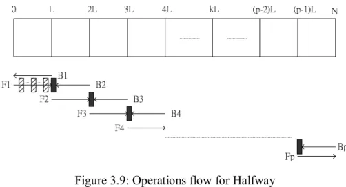
(39) which is L bits long and the metrics calculated are need to be memorized for making the decisions with forward sub-processes. Each backward sub-process is followed by a forward sub-process on the same data block. The required memories for calculation of the decisions are M rd = L × 2 K -1 × q . Different from the first method, the initialization metrics for each backward sub-process are set in a uniform and arbitrary way. The 2 K -1 calculated metrics on the first data of the interval of size L in each backward sub-process are needed to be stored. They will serve as the initialization metrics for the sub-processes starting from the next iteration. The memory capacity for these kind initialization metrics is M ri = D × ( p - 1) × 2 K -1 × q where the first term in right hand side, D , represents the number of the component encoders. Usually, we use two RSC encoders in turbo code, that is D = 2 . The overall required memories are Mtotal = ( L + D × ( p -1) ) × 2K -1 × q for using only one ACS processor and Mtotal = ( L + D × ( p - 2) ) × 2K -1 × q for that with two processors. This method is most effective and fastest in these three memory saving algorithms because there are no initialization processing and processing forcing the convergence of the trellis needed in the operations.. Figure 3.9: Operations flow for Halfway (The rectangles with gray lines are the memories required during making decisions. 29.

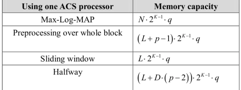
(40) and the black rectangles represent the memories for next-iteration initialization). We take 3GPP Turbo code as an example and assume L = 93 , p = 55 and q = 10 , the memory capacity is. (93 + 2 × ( 55 - 1) ) × 8 ×10 = 16080 = 16.08 Kbits This number is 25 times smaller than the direct decoding method.. 3.2.4 Comparisons The memory capacities for each method are listed in Table 3.1. Because preprocessing over whole block method needs an initialization process over whole block, its speed is slower than those who do not need initializations. The sliding window method also needs several initialization processes over some small windows. According to the length of the block ( L ) and the length of pre-processing ( b ), the sliding windows method may be slower or faster than the first memory saving method but never be faster than Halfway method. If the length of pre-processing is bigger than L , the overlapping calculations of backward metrics occur more times and it will make the decoding speed slow down. Because halfway method needs no initializations, it can perform as faster as the original Max-Log-MAP algorithm.. Using one ACS processor. Memory capacity N × 2 K -1 × q. Max-Log-MAP Preprocessing over whole block. ( L + p - 1) × 2 K -1 × q L × 2 K -1 × q. Sliding window Halfway. ( L + D × ( p - 2) ) × 2. K -1. ×q. Table 3.1: Comparisons of saving memory decoding methods 30.

(41) Assume using only one decoder with only one ACS processor. That is the decoder can only deal with one trellis stage at one time regardless of forward recursion calculations or backward recursion calculations. The following symbols will be used: N. the length of one data frame. K. the constraint length of the convolutional encoder. q. the number of quantization binary digits. L. block length. p. the number of block. b. the length for convergence when using sliding window, b = dL , d Î N. D. the number of the encoders. We will use the subscript “wb” as “whole block”, the subscript “sw” as “sliding window”, the subscript “hw” as “halfway”, POWB as “preprocessing over whole block method”, SW as “sliding window method” and HW as “halfway method”. The comparison of the complexities bases on the same decoding algorithm but different memory saving method. We only need to consider only the numbers of trellis stages required processing. The numbers of stages required processing per half iteration for each method is listed below: POWB: 2 × N + ( N - Lwb ) = 3 × N - Lwb SW: N mod Lsw = 0. ìï2 × N + ( psw - 1) × b if b < Lsw í ïî2 × N + ( psw - d ) × b b = d × Lsw. dÎN. HW: 2 × N The hypothesis N mod Lsw = 0 for SW is an assumption without losing generality. For POWB, the advantages are that it needs fewer memories than direct. 31.

(42) decoding without using any memory saving skills and it also provides the same performance as direct decoding. The disadvantages are the decoding latency and the need for many calculations to initialize the backward initialization memory. For SW, the advantage is that the memory capacity needed is smaller than other methods if let Lsw < Lhw , Lwb . The disadvantage is the need for initializations. If Lsw < Lwb and b ³ Lsw , it will need more calculations of initialization than POWB.. When b ³ Lsw , there will be. ( p - d ) × ( b - Lsw ). overlapping calculations for. initializations. For HW, the advantage is the lack of the initialization; therefore it needs as many calculations as direct decoding does. This is very helpful in using only one ACS processor. The simulation performance of HW in our test is equal to SW. The disadvantage is the memory capacity compared to other memory saving methods. From another aspect, decoding one bit will need to calculate m trellis stages, where m is: mPOWB = mSW. ( 3 × N - Lwb ) = 3 - Lwb. N N 2 × Lsw + b b » = 2+ Lsw Lsw. mHW =. »3. 2× N =2 N. We define efficiency as follows: efficiency =. decode one bit ' s information number of forward and backward state metrics calculated. = m -1 Theoretically, decoding one bit will require one forward state metrics calculation and one backward state metrics calculation. By observing the above definition, we know halfway method provide the same efficiency as the theoretic value and it is the most efficient calculation in these three memory-saving methods. Furthermore, the. 32.

(43) redundant calculations will consume unnecessary power. The comparison curves of the BER performances of the SW and HW method are shown in Figure 3.10. Assume using 3GPP turbo coder, the data frame size N = 500 , LHW = 256 , LSW = 24 and b = 24 . The word “SW-#A-#B” in Figure means the curve uses sliding window method with LSW = # A and b = # B ; the word “HW-#C” means the curve uses halfway method with LHW = # C . Compare halfway and sliding window Frame size=500 Simulation Bits=5*106 Rate=1/3 G=[15,13]octal iteration=5. -1. 10. -2. BER. 10. -3. 10. Floating point Max-Log-MAP SW-24-24 HW-256 -4. 10. 0. 0.5. 1. 1.5. SNR(dB). Figure 3.10: Compare the performances of halfway and sliding window. If using sliding window method with fewer than (d + 1) ACS processors, it will lead to an additional memory of 2 K -1 × q and decrease the decoding speed. The problem of the slow decoding speed of sliding windows method could be solved by using (d + 1) ACS processors. However, the decoder using halfway method only needs an additional ACS processor, totally two ACS processors, can achieve the same decoding speed as the sliding window method with (d + 1) ACS processors.. 33.

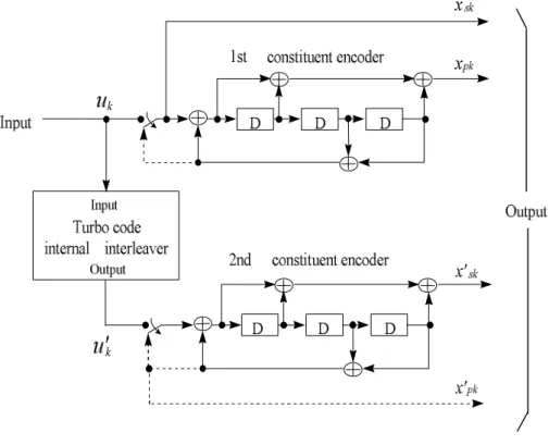
(44) ___________________________________________________. Chapter 4 3GPP Turbo Encoder ___________________________________________________. 3GPP Turbo coder [29] uses Parallel Concatenated Convolutional Code (PCCC) with two 8-state constituent encoders and one internal interleaver. The code rate of Turbo coder is 1/3. The structure of 3GPP Turbo coder is shown in Figure 4.1. The requests of the encoder are as follows: 1. The initial value of the shift registers of the constituent encoders shall be all zeros. 2. Outputs from the Turbo coders are. xs1 , x p1 , x¢p1 ,..., xsK , x pK , x¢pK where xs1 , xs 2 ,..., xsK are the systematic bits which equal to the input bits uk to the Turbo encoder, and K is the number of a block of input bits, and x p1 , x p 2 ,..., x pK and. x¢p1 , x¢p 2 ,..., x¢pK are the bits output from first and second constituent encoders, respectively. The bits output from Turbo code internal interleaver are denoted by u1¢, u2¢ ,..., uk¢ and these bits are to be input to the second constituent encoder.. 4.1 Constituent Encoder 3GPP constituent 8-state encoder and its corresponding trellis diagram are shown in Figure 4.1. The transfer function of the 8-state constituent code for PCCC is: é 1 + D 2 + D3 ù , G ( D) = ê1, 3 ú ë 1+ D + D û 34.

(45) Figure 4.1: Structure of rate 1/3 Turbo coder (dotted lines apply for trellis termination). . S . S . S . S . S . S . S .. S0. 1. constituent encoder D0. D1. D2. 0/00 1/11 1/11 0/00. 2. 1/10 0/01. 3. 0/01 1/10. 4. 0/01 1/10 1/10. 5. 0/01. 6. 1/11 0/00. 7. 0/00 1/11. .S .S .S .S .S .S .S .S. 0. 1. 2. 3. 4. 5. uk/xsk,xpk S0 = 000 S1 = 001 S2 = 010 S3 = 011 S4 = 100 S5 = 101 S6 = 110 S7 = 111 register states D0D1D2. uk=0 Dotted line: uk=1 Solid line :. 6. 7. Figure 4.2: Constituent encode of 3GPP turbo encoder and its trellis. 35.

(46) 4.2 Trellis Termination Because the first request, the initial value of the shift registers of the encoders shall be all zeros, both the constituent encoders need to perform trellis termination after encoding one block of input bits. The action of terminating the trellis is performed by taking the last K - 1 bits from the shift register of each encoder feedback to their selves after all information bits are encoded then all shift registers will return to zero. The switch in each constituent encoder should be switched to the lower position when terminating and the structure of each encoder is shown in Figure 4.3. These encoded tail bits are padded after the encoded information bits, and the transmitted bits for trellis termination shall be:. xs( K +1) , xp( K +1) , xs(K +2) , xp( K +2) , xs( K +3) , xp( K +3) , xs¢(K +1) , x¢p( K +1) , xs¢( K +2) , x¢p( K +2) , xs¢( K +3) , x¢p( K +3). Figure 4.3: Constituent encoder for terminating the trellis. 4.3 Interleaver The 3GPP Turbo code internal interleaver is a block interleaver consisting of a rectangular matrix and its size is decided by the frame size of the input bits, K. The original message bits input to the interleaver row by row. If the input bits are not enough to filling the matrix, we need to add some redundant bits to fill it. Then we perform intra-row permutations and inter-row permutations of the rectangular matrix. Finally, the bits in the matrix are read out column by column and pruning the 36.

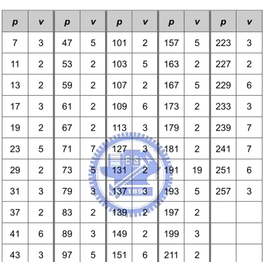
(47) redundant bits we added before. We denote the bits input to the internal interleaver by. u1 , u2 , u3 ,...uK , where K is the integer number of the bits and takes one value of 40 £ K £ 5114.. 4.3.1 Deciding the size of the rectangular matrix First to all, we need to decide the number of the rows and the columns of the rectangular matrix according the following process: (1) According to the equation (33), determining the number of rows of the rectangular matrix, R. The rows of rectangular matrix are numbered 0, 1, …, R - 1 from top to bottom. ì 5, if (40 £ K £ 159) ï R = í 10, if ((160 £ K £ 200) or ( 481 £ K £ 530)) ïî 20, if ( K = any other value). (33). (2) Along with Table 4.1 and relationship shown below, we can determine the prime number, p, used in the intra-permutation and the number of columns of rectangular matrix, C. The columns of rectangular matrix are numbered 0, 1, …, C - 1 from left to right if (481 £ K £ 530) then p = 53 and C = p. else Find minimum number p from Table 4.1 such that. K £ R ´ ( p + 1) , and determine C such that. 37.

(48) K £ R × ( p - 1) ì p - 1 if ï C = íp if R × ( p - 1) < K £ R × p ï p + 1 if R× p £ K î end if. p. v. p. v. p. v. p. v. p. v. 7. 3. 47. 5. 101. 2. 157. 5. 223. 3. 11. 2. 53. 2. 103. 5. 163. 2. 227. 2. 13. 2. 59. 2. 107. 2. 167. 5. 229. 6. 17. 3. 61. 2. 109. 6. 173. 2. 233. 3. 19. 2. 67. 2. 113. 3. 179. 2. 239. 7. 23. 5. 71. 7. 127. 3. 181. 2. 241. 7. 29. 2. 73. 5. 131. 2. 191. 19. 251. 6. 31. 3. 79. 3. 137. 3. 193. 5. 257. 3. 37. 2. 83. 2. 139. 2. 197. 2. 41. 6. 89. 3. 149. 2. 199. 3. 43. 3. 97. 5. 151. 6. 211. 2. Table 4.1: List of prime number p and associated primitive root v (3)Write the input bit sequence u1 , u2 , u3 ,...u K into the R ´ C rectangular matrix row by row: y2 y3 é y1 êy y(C + 2) y(C +3) ê (C +1) êM M M ê ëê y(( R-1)×C +1) y(( R -1)×C + 2) y(( R -1)×C +3). L L L L. yC ù y2C úú M ú ú yR×C ûú. where yk = uk for k = 1, 2, …, K and if R ´ C > K, the dummy bits are added to the 38.

(49) tail of the input sequence such that yk = 0 or 1 for k = K + 1, K + 2, …, R´ C. These dummy bits will be discarded when read the bits from the rectangular matrix after intra-row and inter-row permutations.. After the R´ C rectangular matrix is filled with the input and dummy bits, we perform the intra-row permutations and inter-row permutations in turn. Inter-row. permutation. patterns. Number of input bits K Number of rows R <T(0), T(1), …, T(R - 1)> (40≦K≦159). 5. <4, 3, 2, 1, 0>. 10. <9, 8, 7, 6, 5, 4, 3, 2, 1, 0>. (160 ≦ K ≦ 200) or (481≦K≦530) (2281 ≦ K ≦ 2480) or (3161≦K≦3210). <19, 9, 14, 4, 0, 2, 5, 7, 12, 18, 16, 20 13, 17, 15, 3, 1, 6, 11, 8, 10> <19, 9, 14, 4, 0, 2, 5, 7, 12, 18, 10, 8,. K = any other value. 20 13, 17, 3, 1, 16, 6, 15, 11>. Table 4.2: Inter-row permutation patterns for Turbo code internal interleaver. 4.3.2 Intra-row and inter row permutations After the bits input to the R ´ C rectangular matrix, the intra-row and inter-row permutations for the R´ C rectangular matrix are performed stepwise by using the following algorithm with steps (1) – (6): (1) Select a primitive root v from Table 4.1, which is indicated on the right side of the prime number p. (2) Construct the base sequence. s( j ). jÎ{0,1,L, p - 2}. 39. for intra-row permutation as:.

(50) s ( j ) = ( v × s ( j - 1) ) mod p ,. j = 1, 2, L , ( p - 2) , and s(0) = 1.. (3) Assign q0 = 1 to be the first prime integer in the sequence determine the prime integer qi in the sequence. qi. qi. iÎ{0,1,..., R -1}. , and. to be a least. iÎ{0,1,..., R -1}. prime integer such that g .c.d (qi , p - 1) = 1 , qi > 6 , and qi > qi -1 for each i = 1, 2,L , R - 1 .. Here g.c.d. is greatest common divisor.. (4) Permute the sequence. qi. iÎ{0,1,..., R -1}. to make the sequence. ri. iÎ{0,1,L, R -1}. such. that rT (i ) = qi , i = 0,1,L , R - 1 where T (i). iÎ{0,1,L, R -1}. is the inter-row permutation pattern defined as the one. of the four kind of patterns, which are shown in Table 4.2, depending on the number of input bits K. (5) Perform the i-th (i = 0, 1, …, R - 1) intra-row permutation as: if (C = p) then U i ( j ) = s(( j ´ ri ) mod( p - 1)) ,. j = 0, 1, …, (p - 2), and Ui(p - 1) = 0,. where Ui(j) is the original bit position of j-th permuted bit of i-th row. end if if (C = p + 1) then U i ( j ) = s(( j ´ ri ) mod( p - 1)) ,. j = 0, 1, …, (p - 2).. Ui(p - 1) = 0, and Ui(p) = p,. where Ui(j) is the original bit position of j-th permuted bit of i-th row, and if (K = R ´ C) then Exchange UR-1(p) with UR-1(0). end if end if if (C = p - 1) then 40.

(51) U i ( j ) = s(( j ´ ri ) mod( p - 1)) - 1 ,. j = 0, 1, …, (p - 2),. where Ui(j) is the original bit position of j-th permuted bit of i-th row. end if (6) Perform the inter-row permutation for the rectangular matrix based on the pattern T (i ). iÎ{0,1,L, R -1}. , where T(i) is the original row position of the i-th. permuted row.. 4.3.3 Output the bits from the rectangular matrix with pruning After intra-row and inter-row permutations, the bits of the permuted rectangular matrix are denoted by y 'k : é y '1 y '( R+1) y '(2 R +1) êy' ê 2 y '( R+ 2) y '(2 R + 2) êM M M ê y '3 R ë y 'R y '2 R. L L L L. y '((C -1)× R +1) ù y '((C -1)× R + 2) úú ú M ú y 'C ×R û. The output of the Turbo code internal interleaver is the bit sequence read out column by column from the intra-row and inter-row permuted R ´ C rectangular matrix starting with bit y'1 in row 0 of column 0 and ending with bit y'CR in row R - 1 of column C - 1.. The output is pruned by deleting dummy bits that were padded to. the input of the rectangular matrix before intra-row and inter row permutations, i.e. bits y'k that corresponds to bits yk with k > K are removed from the output.. The bits. output from Turbo code internal interleaver are denoted by x'1, x'2, …, x'K, where x'1 corresponds to the bit y'k with smallest index k after pruning, x'2 to the bit y'k with second smallest index k after pruning, and so on. The number of bits output from Turbo code internal interleaver is K and the total number of pruned bits is: R × C - K . The interleaving flow chart after deciding R, C is shown in Figure 4.4.. 41.

(52) Figure 4.4: Interleaving flow chart. 42.

(53) _____________________________________________________________________. Chapter 5 Design Considerations _____________________________________________________________________. The 3GPP turbo encoders are constructed by two identical encoders; therefore, we can use only one decoder to decode the received sequence serially and iteratively. In this thesis, the turbo decoder uses only one decoder and only one ACS processor to calculate the forward and backward state metrics for low complexity. When designing the hardware of the decoder, we need to discuss and consider about several issues as follows: 1. Decoding algorithm selection. 2. Memory saving method selection. 3. Decision of the block length. 4. The analyses of fixed-point representations for calculations.. 5.1 Decoding algorithm selection Due to Max-Log-MAP algorithm’s low complexity and only minor performance loss comparing with Log-MAP and the poor SNR sensitivity which means we will not need any multiplications in decoding process, we implement our hardware by Max-Log-MAP algorithm.. 5.2 Memory saving method selection Because we use only one decoder for decoding, we cannot tolerate the redundant. 43.