在因子關聯結構模型下用高效率權重取樣估計聯合違約機率

!

#

$

%

&

'

"

()'*+,"

-

"

.

"

/

"

0

"

123456789:;<="

>?@ABC)5DEFG>"

"

HIIJKJLMN"OPQRSNTMKL"UTPQVJMW"JM"HXNJPTNJRM"RI" "

YLITZVN"[SR\T\JVJN]"ZM^LS"_TKNRS"`RQZVT"aR^LVX"

"

"

"

*" +" bcde'"

fghicjkl" " hi"

" " " " " " " " " " mno" " hi"

"

"

p" q" r" !" s" t" u" v" w " x"

"

"

123456789:;<=>?@ABC)5DEFG>"

HIIJKJLMN"OPQRSNTMKL"UTPQVJMW"JM"HXNJPTNJRM"RI" "

YLITZVN"[SR\T\JVJN]"ZM^LS"_TKNRS"`RQZVT"aR^LVX"

"

"

"

"

"

*" +" bcde'" " " " " " " " " " UNZ^LMNcyTM"zXZL{"|LL"

fghicjkl" " " " " " " " " " }^~JXRSc`{ZTM•zXJTMW"zTM"

" " " " " " " " " " " " " mno" " " " " " " " " " " " " " " " " " zZJ•€JLM"zZMW"

"

"

!" #" $" %" &" '"

()'*+,"

-" ." /" 0"

"

"

"

"

pqr!stuvwx"

"

123456789:;"

<=>?@ABC)5DEFG>"

*+bc

fghi

!#$%&'()'*+,"

‹

" " " " " "

Œ

"

"

"

"

"

"

"

"

"

"

"

"

"

"

"

"

"

HIIJKJLMN"OPQRSNTMKL"UTPQVJMW"JM"HXNJPTNJRM"RI" "

YLITZVN"[SR\T\JVJN]"ZM^LS"_TKNRS"`RQZVT"aR^LVX"

UNZ^LMNÞ"

}^~JXRS

OMXNJNZNL"RI"UNTNJXNJKX"

€TNJRMTV"`{JTR"•ZMW"‚MJ~LSXJN]"

"

}\XNSTKN"

"

Importance sampling is a commonly used technique to improve Monte Carlo methods, especially in working with rare events. It is designed to increase the probability of sampling from rare events and is therefore well-suited for estimating default related items in various products given the rarity of default events. It is also simple to implement and versatile in that in can be easily extended to estimate different items. But the main challenge is selecting an importance sampling scheme that not only increases the probability of rare events but also effectively reduces the variance of the estimate. Under the multivariate framework when multiple entities are involved, variance reduction becomes even more challenging as there is no closed form solution for such optimization problem. In this study, we propose an effective importance sampling algorithm that both increases the probability of rare events and reduce variance of estimates. We consider the problem of variance reduction under the framework of Large Deviation Theory, and establish an efficient importance sampling estimator that can be applied to evaluating default events. Then we extend this importance sampling scheme to another popular type of default event and incorporate it into a conditional importance sampling scheme. Our numerical results confirm that the proposed algorithms for direct importance sampling and conditional importance sampling are more efficient in terms of variance reduction. Our algorithms are overall more robust under different specified initial conditions.

ßà

I am thankful for the opportunity to study at NCTU these past two years. I want to first thank Dr. Chung-Hsiang Han for being my advisor and very thoroughly guiding me on my thesis. Without his help, I could not have finished this research project. He has been very patient in teaching me the basics of quantitative finance step by step all the way to helping me

understand current research topics in the field of credit risk modeling. He also provided me the opportunity to intern at the futures trading department in ChinaTrust, which turned out to be an extremely valuable experience. Now I not only understand the basics of

continuous-time finance but also appreciate how such tools are used in industry. It is my pleasure and privilege to have studied under Dr. Han. I also want to thank my co-advisor Dr. Hui-Nien Hung for giving me valuable research tips. As an experienced practitioner and researcher in many fields of statistics, Dr. Hung gave me valuable career advice. Finally, I want to thank my church for giving me the opportunity to serve in college ministry here in NCTU and NTHU. I thoroughly enjoyed the experience and wish I can stay here longer. Lastly, I want to thank all my friends and family for supporting me and always encouraging me. I could not have survived these past two years without these precious people in my life.

Table of Contents

1 Introduction and Motivation 1

2 Characterization of Default Time 3

2.1 Default Time of a Single Firm . . . 3

2.2 Brief Introduction to Copula Function . . . 4

2.3 Joint Default Time Under Gaussian and Student-T Copula . . . 5

2.4 Covariance Matrix under Gaussian Factor Copula Model . . . . 8

3 Estimating Joint Default Probability 10 3.1 Basic Monte Carlo Method . . . 12

3.2 Brief Review of Importance Sampling . . . 12

3.3 Importance Sampling Problem Description . . . 13

4 Importance Sampling in Large Deviation Theory 16 4.1 Efficient Importance Sampling . . . 16

4.2 Applying Results of Large Deviation Theory . . . 17

4.3 Efficiency under Gaussian Factor Copula . . . 20

5 Application I: Joint Default Probability 26 5.1 Under Gaussian Copula . . . 26

5.2 Under Student-T Copula . . . 27

5.3 Numerical Comparison . . . 29

6 Application II: Basket Default Swap 35 6.1 Introduction to Basket Default Swaps . . . 35

6.2 Algorithms under Gaussian Copula . . . 37

6.2.1 Basic Monte Carlo Method . . . 37

6.2.3 Conditioning on the Common Factor . . . 42

6.2.4 Direct Importance Sampling . . . 44

6.2.5 Numerical Comparison . . . 45

6.3 Algorithms under Student-T Copula . . . 51

6.3.1 Basic Monte Carlo Method . . . 51

6.3.2 Conditional Importance Sampling . . . 52

6.3.3 Numerical Comparison . . . 54

7 Conclusion 58 Reference . . . 60

List of Tables

5.1 Estimating Joint Default Probability with Different Default

Thresh-old under Gaussian Copula . . . 31

5.2 Estimating Joint Default Probability with Different Number of Firms under Gaussian Copula . . . 32

5.3 Estimating Joint Default Probability with Different Default Thresh-old under Student-T Copula . . . 33

5.4 Estimating Joint Default Probability with Different Number of Firms under Student-T Copula . . . 34

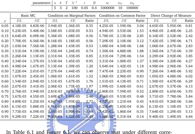
6.1 Estimating DL under Different Correlation Strengths . . . 46

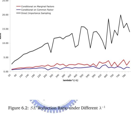
6.2 Estimating DL under Different Default Intensity . . . 49

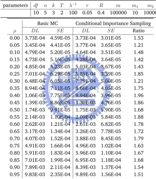
6.3 Evaluating DL with Different Correlation Strengths . . . 55

6.4 Evaluating DL with Different Default Intensity . . . 56

List of Figures

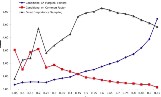
6.1 SE Reduction Ratio under Different ρ . . . 47

Chapter 1

Introduction and Motivation

Effectively estimating default probability in credit derivatives has been an area of ongoing research. The problem starts with the characterization of default time. There are two main approaches: structural form and reduced form. Structural form models the asset and debt value of the company. It treats them as a first passage time problem and considers default to occur when asset value of the firm falls below the debt value. Merton [17] (1974) first proposed this model and later Black and Cox [1] (1976), Geske [9] (1977), Leland [16] (1994), Longstaff and Schwartz [15] (1995), and Zhou [18] (2001)also followed this line of thinking. They mainly worked with default of a single firm. Only Zhou [18] (2001) modeled default of two firms with two corre-lated brownian motions and derived closed form solution to the joint default probability of the two firms. His results, however cannot be easily extended to more firms. Hull and White [11] (2001) shows how multiple firms can be dealt with using Monte Carlo methods. Typically, evaluating such models requires computationally intensive numerical procedures.

Reduced form models on the other hand treats default as exogenous. It bypasses the particular firms captical structure and uses available market in-formation to model defaults. Schönbucher [19] (2003), Duffie [7] (2003), and Lando [12] (2003) are a few main proponents of this approach. Up to now, the industry standard follows the reduced form’s line of thinking. Li [13] (2000) first developed the copula approach to develop the correlation structure among default times and Laurent and Gregory [10] (2005) later ex-tended it and represented the correlation structure in factor form, also known as factor-copula approach. We will follow the industry standard and adopt

the factor copula approach in this study.

Once default time is characterized, we can utilize the model to now eval-uate joint default probability and various credit derivatives. Basket Default Swaps (BDS) is a common type of multi-name credit derivatives along with Collaterized Debt Obligations (CDO). Chiang, Yueh, and Hsieh [5] (2007) proposed an efficient algorithm for valuing BDS (hereafter as CYH). Their

study proposes an efficient algorithm to evaluate kth _{to default BDS. It adopts}

the factor copula approach to modeling default time and mainly works with Gaussian copula. In this study, we generalize their study and consider joint

default probability along with kth _{to default BDS under both Gaussian and}

Student-T copula. We propose another algorithm that is more efficient and approach the problem of variance reduction from the perspective of Large Deviation Theory. Large Deviation Theory is an active area of applied proba-bility that mainly focuses on behavior of extremal events. We use results from Large Deviation Theory to solve the problem of variance reduction for our estimation algorithm.

Chapter 2

Characterization of Default Time

2.1 Default Time of a Single Firm

We characterize distribution of a firm’s default time τ in terms of its hazard rate function h(.). Here we briefly review the definition and relationship be-tween survival function, hazard function and CDF.

Definition 2.1 (survival function). If τ is the default time of a firm with CDF F , then S(t) = P(τ > t) = 1 − F (t) is the survival function of τ.

Definition 2.2 (hazard rate function). Suppose the default time τ has density

function f(t) and survival function S(t), then the hazard rate function h(t) is defined as

hτ(t) =

fτ(t)

Sτ(t)

.

Hazard rate function is useful for understanding probability of a firm’s default immediately after time t, given that it has survived up to time t. We can understand hazard rate function in the following conditional probability.

Given a firm has survived t years, the probability it will default in the coming time interval ∆t can be written as follows:

P(τ ∈ (t, t + ∆t)|τ > t) = P(τ ∈ (t, t + ∆t))_{P(τ > t)} ≈ f (t)∆t

1_{− F (t)} = h(t)∆t. (2.1) We can see that this probability can be approximated by the value of hazard rate function at time t times a small time increment ∆t.

According to definition 2.2, we can write the distribution function in terms of the hazard rate function:

F (t) =P(τ ≤ t) = 1 − exp ! − " t 0 h(s)ds # (2.2) Equation (2.2) shows that with effective estimation of hazard rate, we can model distribution of default time. According to Cherubini, Luciano and Vecchiato [4] (2004), the hazard rate function can be obtained in several ways:

• From historical default rates provided by rating agencies.

• By using the Merton approach according to Delianedis and Geske [6]

(1998).

• Extracting default probabilities by using market observable information,

such as asset swap spread, CDS spread or corporate bond prices accord-ing to Li [14] (1998).

We will not focus on methods of extracting hazard rate function in this study. A typical assumption is that the hazard rate is a constant λ. In this case, default time τ follows an exponential distribution with intensity λ. Here and on, we will use this assumption. This implies:

F (t) =P(τ ≤ t) = 1 − exp(−λt) (2.3)

2.2 Brief Introduction to Copula Function

We have characterized default time of a single firm, and now proceed to combine default time distributions of different firms into a joint distribution through copula functions. First, we give a brief introduction to copula func-tions.

Definition 2.3 (copula function). A n-dimensional copula C is a real-value

function with range I = [0, 1] and domain In _{such that}

• C(u) is increasing in every component uk, k = 1, 2 · · · n, called n-increasing.

• For every u ∈ In_{, C(u) = 0 if u}

k= 0 for some k, and C(u) = ukif ui = 1,

• For all a,b ∈ In _{with a ≤ b in every component, then the n-box B =}

[a1, b1]· [a2, b2]· · · · [an, bn] satisfies Vn(B)≥ 0, where Vnis the n-volume.

Copula function, C, can be intrinsically understood as a multivariate dis-tribution function with uniform marginal disdis-tributions.

C(u1, ..., un) =P (U1 ≤ u1,· · · , Un≤ un)

Let F be n-dimensional distribution with F1, ..., Fnas the univariate marginal

distributions. Note that ui = Fi(xi) is uniform on [0, 1] for i = 1, ..., n. The

copula function can combine these uniform marginals u1, ..., un into a

multi-variate distribution function. By probability integral transformation, we can write,

C(F1(x1),· · · , Fn(xn)) =P(U1 ≤ F1(x1),· · · , Un≤ Fn(xn))

=P(F₁−1(U1)≤ x1,· · · , Fn−1(Un)≤ xn)

=P(X1 ≤ x1,· · · , Xn≤ xn)

= F (x1,· · · , xn)

, where Sklar theorem guarantees the converse.

Theorem 2.1 (Sklar 1959). Let F be an n-dimensional multivariate distribution function with marginal distributions F1(·), · · · , Fn(·). Then there exists an

n-dimensional copula function C such that

F (x1,· · · , xn) = C(F1(x1),· · · , Fn(xn)).

Furthermore, if F1(·), · · · , Fn(·) are continuous, then C is unique.

Therefore, if we know marginal distributions F1, ..., Fnthen we can specify

the copula function and joint distribution.

2.3 Joint Default Time Under Gaussian and

Student-T Copula

Now we have characterized default time of a single firm. We will combine default time distributions of several firms into a joint distribution through

copula functions. We will focus on Gaussian and Student T copula functions and provide algorithms for generating joint default time according to these two copula functions.

Now suppose there are n firms, and as mentioned before, we assume the

default time τi of each each firm follows an exponential distribution with

in-tensity λi for i = 1, ..., n. Let Fi(.) be the distribution function of default time

τi for firm i, i = 1, ..., n. The main purpose of using copula function here is

to generate a set of correlated uniform variates (U1, ..., Un) according to the

specified copula correlation structure. Next, we use the correlated uniform variates generated from the copula function to compute default time for each individual firm through inverse mapping of the firm’s default time distribution i.e. τi = Fi−1(Ui) for i = 1, ..., n.

General Form of Gaussian Copula

C(u1, u2,· · · , un; Σ) = ΦΣ(Φ−1(u1), Φ−1(u2),· · · , Φ−1(un))

where ΦΣ(.) is the standardized multivariate normal distribution with

covariance matrix Σ and Φ(.) is CDF of N(0, 1). In this case, given ui =

Fi(τi), where Fi(.) is default time distribution of firm i, we can rewrite

the Gaussian copula function as follows,

C(F1(τ1),· · · , Fn(τn); Σ) = ΦΣ(Φ−1(F1(τ1)),· · · , Φ−1(Fn(τn)))

We can sample joint default time from a Gaussian copula as follows:

Algorithm 2.1 (Joint default time under Gaussian copula).

1. Given Σ, generate correlated uniform variates (U1, ..., Un) from the

Gaus-sian Copula function.

(1) Find the Cholesky decomposition A of Σ such that: Σ = AAT_.

(2) Generate n independent random variables Z = (Z1,· · · , Zn)T from

N (0, 1).

(3) Let X = (X1, ..., Xn)T = AZ. Now we know W ∼ ΦΣ(.)

2. Use correlated uniform variates (U1, ..., Un) generated from Gaussian

Copula to compute default time through inverse mapping of the firm’s default time distribution.

(1) Let (U1, ..., Un)T = (F1(τ1), ..., Fn(τn))T.

(2) Let τi = Fi−1(Ui), i = 1,· · · n.

General Form of Student-T Copula C(u1, u2,· · · , un; Σ, ν) = TΣ,ν

$

t−1_ν (u1), t−1ν (u2),· · · , t−1ν (un)

%

where TΣ,ν(.) is the standardized multivariate Student-T distribution

with covariance matrix Σ and degrees of freedom, ν. tv(.) is CDF of

univariate Student-T with ν degrees of freedom. In this case, given

ui = Fi(τi), where Fi(.) is default time distribution of firm i, we can

rewrite the Student-T copula function as follows,

C(F1(τ1),· · · , F1(τn); Σ, ν) = TΣ,ν

$

t−1_ν (F1(τ1)),· · · , t−1ν (Fn(τn))

% We can sample joint default time from a Student-T copula as follows:

Algorithm 2.2 (Joint default time under Student-T copula).

1. Given Σ, generate correlated uniform variates (U1, ..., Un) from

Student-T copula function.

(1) Find the Cholesky decomposition A of Σ such that Σ = AAT_.

(2) Generate n independent random variables Z = (Z1,· · · , Zn)T from

N (0, 1).

(3) Generate χ2

ν, a Chi-square variable with d.f.=ν.

(4) Let X = AZ. Then X ∼ N(0, Σ). (5) Let S = (S1, ..., Sn)T = X/

&

χ2

ν/ν. Then S ∼ TΣ,ν(.)

(6) Let Ui = t−1ν (Si) for i = 1, ..., n.

2. Use correlated uniform variates (U1, ..., Un) generated from Student-T

copula to compute default time through inverse mapping of the firm’s default time distribution.

(1) Let (U1, ..., Un)T = (F1(τ1), ..., Fn(τn))T.

2.4 Covariance Matrix under Gaussian Factor

Cop-ula Model

We have shown how to determine joint default time using Gaussian and Student-T copula functions. But we haven’t discussed the exact structure of correlation which is mainly determined by the covariance matrix Σ. To deter-mine Σ, n(n−1)/2 variables need to be estimated, which is extremely difficult when n is large. Laurent and Gregory [10] (2004) proposes the factor model which greatly reduces the number of variables by using two types of factors to intuitively explains firms’ behavior in terms of economic trend and

idiosyn-cratic movements. It reduces complexity from O(n2_{) to O(n) Therefore, we}

adopt the factor model proposed by Laurent and Gregory for determining Σ. Under this model,

Xi = ρiZ0+

' 1_{− ρ}2

iZi, i = 1, 2,· · · , n, (2.4)

where Z0,· · · , Zn are i.i.d. N(0, 1) and ρ1, ..., ρn&[0, 1] Let X = [X1, ..., Xn]T,

then X =       X1 X2 ... Xn      =       ρ1 & 1− ρ2 1 ρ2 & 1_{− ρ}2 2 ... ... ρn & 1− ρ2 n               Z0 Z1 Z2 ... Zn        

The factor loading ρi determines how strongly the ith factor is correlated

to the common factor Z0. Both Z0 and Zi are N(0, 1), and the constraints

posed on on factor loadings ensure that every factor Xi is N(0, 1).

We can see that X has multivariate normal distribution N(0, Σ) where

Σ =         1 ρ1ρ2 ρ1ρ3 · · · ρ1ρn 1 ρ2ρ3 · · · ρ2ρn ... ... 1 ρn−1ρn 1        

Suppose Xi represents firm i, one can intuitively understand Z0 as the

common factor such as certain macroeconomic or industry condition that af-fects all firms in a similar fashion, and Zias the firm specific factors that affect

only the particular firm. Hence we call Z0 the common factor, and each Zithe

Chapter 3

Estimating Joint Default

Probability

Now that we have characterized joint default time distribution, we proceed to formulate the problem of estimating joint default probability. Given time T, we wish to know the probability of all the firms defaulting sometime before T. i.e. we wish to evaluate the following,

p =P (τ1 ≤ T, ..., τn ≤ T ) = E . I(τ1≤T,...,τn≤T ) / =E 0 _n 1 i=1 I(τi≤T ) 2 (3.1) Direct computation of this probability is equivalent of evaluating the CDF of default time (τ1, ..., τn) at (T, ..., T )

p = F (T, ..., T )

But this often involves evaluation of a complex multiple integral that has no closed form solution. One can then resort to numerical methods. But this integration suffers from curse of dimensionality, causing the accuracy of nu-merical integration to decrease significantly as dimension n increases. The integral takes the following forms under Gaussian and Student-T copula. As

mentioned above, here we denote Fi(.) for i = 1, ..., n as default time

distri-bution for firm i.

Recall in Algorithm 2.1, given X = (X1, ..., Xn) ∼ N(0, Σ) and Xi ∼

N (0, 1) for i = 1, ..., n, we can generate default time as τi = Fi−1(Φ(Xi))

for i = 1, ..., n. Then we can also write,

{τi ≤ T } = . F_i−1(Φ(Xi))≤ T / =.Xi ≤ Φ−1(Fi(T )) /

This means joint default probability becomes a problem of calculating

the multivariate normal CDF, ΦΣ(.),

p = ΦΣ(φ−1(F1(T )), ..., φ−1(Fn(T ))) (3.2) = " φ−1(F1(T )) −∞ · · · " φ−1(Fn(T )) −∞ 1 (2π)n2|Σ| 1 2 exp 3 −1 2x T_Σ−1_x 4 dx1...dxn

Under Student-T Copula

Recall in Algorithm 2.2, given S = (S1, ..., Sn)∼ TΣ,ν and Si ∼ tν for i =

1, ..., n, we can generate default time as τi = Fi−1(tν(Si)) for i = 1, ..., n.

Then we can also write,

{τi ≤ T } = . F_i−1(tν(Si))≤ T / =.Si ≤ t−1ν (Fi(T )) /

This means joint default probability becomes a problem of calculating

the multivariate Student-T CDF, TΣ,ν(.),

p = TΣ,ν(t−1ν (F1(T )), ..., t−1ν (Fn(T ))) (3.3) = " t−1ν (F1(T )) −∞ · · · " t−1ν (Fn(T )) −∞ Γ$ν+n 2 % |Σ|12 Γ$ν 2 % (vπ)n2 3 1 + 1 vx T_Σ−1_x 4−ν+n2 dx1...dxn

One can easily observe that evaluation of these two integrals is very dif-ficult, especially when n is large. For our purpose, n is usually larger than 5, which rules out numerical integration as a practical approach. Therefore, we approach the problem with Monte Carlo methods. In this study, we focus on Basic Monte Carlo (Basic MC)and importance sampling methods. In liter-ature, Genz and Bretz [8] (1999) has proposed Quasi Monte Carlo methods (Quasi MC), which is widely adopted as the main numerical method when n is large.

3.1 Basic Monte Carlo Method

Basic MC method is simple to implement. Based on the law of large numbers, the joint default probability can be approximated by its sample mean when m is sufficiently large, p =E 0 _n 1 i=1 I(τi≤T ) 2 ≈ 1 m m 5 j=1 n 1 i=1 I(τi,j≤T )

where τ1,j, ..., τn,j for j = 1, ..., m are m samples of τ1, ..., τn. Based on the

above, we just need to generate m samples for τ1, ..., τn according to

Algo-rithm 2.1 for Gaussian copula and AlgoAlgo-rithm 2.2 for Student-T copula and then evaluate the indicator function for our m samples. However, default event for highly ranked firms is typically very rare, causing default times of

n firms to all be less than or equal to T an extremely rare event. This makes

Basic MC method inaccurate. Therefore we modify the Basic MC method with importance sampling techniques to improve accuracy of our estimation.

3.2 Brief Review of Importance Sampling

Importance sampling is a commonly used tool for rare event simulation. The basic idea is to change the original probability measure P to a new probability measure ˜P that puts more weight on the rare event we want to sample. With a good choice of ˜P, we can increase the simulation efficiency by generating more desired samples as well as reducing variance.

Suppose we want to estimate

θ =E[h(X)] =

"

Rn

h(x)f (x)dx (3.4)

where X = [X1,· · · , Xn]T is a random vector in Rnwith a joint density f(x) =

f (x1,· · · , xn). Basic Monte Carlo Method gives us the following estimate

ˆ θ = 1 m m 5 i=1 h$X(i)%, (3.5)

where every X(i) _{for i = 1, ..., m are i.i.d. samples from probability measure}

If we find it ineffective to sample from Pf(.), we can sample from another

probability measure, call it Pg(.) with density g(.), which is absolute

continu-ous with respect to f(.). Then we can write the following,

θ = " Rn h(x)f (x)dx = " Rn h(x)f (x) g(x) g(x)dx =Eg 6 h(Y )f (Y ) g(Y ) 7 , (3.6)

where the random vector Y has the density g(·). Now our original estimator ˆ θ is replaced by ˆ θ = 1 m m 5 i=1 h$Y(i)%_f$_Y(i)% g (Y(i)₎ , (3.7)

where the random samples are taken from g(·). The weight f (Y(i)₎

g(Y(i)₎ is called

the likelihood ratio or Radon-Nikodym derivative evaluated at Y(i)_{. For}

no-tational simplicity, here and on, we will denote Radon-Nikodym derivative in the following fashion dPf

dPg,

dPf

dPg

(Y ) = f (Y )

g(Y )

Our goal is twofold: 1)Find an appropriate measure g(.) such that g(Y ) >>

f (Y ) on important regions. This will increase probability of generating rare

samples from those regions we are interested in, 2) Find g(.) that minimizes variance of importance sampling estimator, V ar(ˆθ).

3.3 Importance Sampling Problem Description

Having established the basic notion of importance sampling, we now proceed to formulate our importance sampling scheme. We will consider importance sampling under Gaussian copula first and then apply the results to Student T copula. Under Gaussian copula, we know that for i = 1, ..., n,

{τi ≤ T } = . F_i−1(Φ(Xi))≤ T / =.Xi ≤ Φ−1(Fi(T )) / Then we can write,

p = E 0 _n 1 i=1 I(τi≤T ) 2 =E 0 _n 1 i=1 I(Xi≤Φ−1(Fi(T )) 2

Recall that X = [X1, ..., Xn]T is multivariate normal N(0, Σ). We need to

employ importance sampling when Φ−1_(F

i(T )) is very negative, i.e. when T

is very small or when intensity λi of default time distribution for firm i is very

small, which is often the case. We can generalize the problem in the following way. Given some D = [d1, ..., dn]T where d1, ..., dn ∈ R, we wish to instead

evaluate, p = E 0 _n 1 i=1 I(Xi≤di) 2 =E {I(X ≤ D)}

Here X ≤ D means elements of X are less than elements of D i.e. X1 ≤

d1, ..., Xn ≤ dn. We will use this notation from here and on. Recall that

we can use the Basic MC to approximate p. However, Basic MC simulation with random variable X ∼ N(0, Σ) under P(.) is inaccurate when D is small. Therefore, we consider importance sampling with Y ∼ N(u, Σ) under new

measure Pu(.) in approximating p. Our goal is to find u that will minimize

variance of our importance sampling estimator.

Under new measure Pu(.)

p = Eu ! I(Y≤D) dP dPu # (3.8)

With Y(j) _{∼ N(u, Σ) as i.i.d. samples from P}

u, the importance sampling

esti-mator will be ˆ p = 1 m m 5 j=1 I(Y(j)_≤D) dP dPu (3.9)

Note that ˆp is an unbiased estimator because Eu_{{ˆp} = p. Since ˆp is the average}

of m i.i.d samples, its variance will be 1

m times the variance of

8 I(Y≤D)ddPPu 9 , V ar(ˆp) = 1 m : Eu 03 I(Y≤D) dP dPu 422 − p2 ; (3.10) To minimize V ar(ˆp), we just need to optimize with respect to u the second moment of I(Y≤D)ddPPu. F (u) :=Eu 03 I(Y≤D) dP dPu 422 (3.11) Such optimization problem is extremely complicated because Y is multivari-ate, and currently there is no closed form solution for F (u). But we can

approach the problem of variance reduction from the framework of Large De-viation Theory, and find a asymptotic minimizer that can reduce the second moment, F (u), and hence reduce variance. This will produce efficient impor-tance sampling asymptotically. We will define this in the next chapter.

Chapter 4

Importance Sampling in Large

Deviation Theory

4.1 Efficient Importance Sampling

First we need to establish the notion of efficient importance sampling in Large Deviation Theory . We reformulate the problem by introducing a scaling factor

−√L that will later allow us to apply results from Large Deviation Theory.

Let D = −√LC = ₋√L[c1,· · · , cn]T, where c1,· · · , cn are positive constants.

Now, we rewrite p and F (u) as pL and FL(u). Under P(.) Let X(i) ∼ N(0, Σ)

for i = 1, ..., L be i.i.d samples from P(.), then we know _√1

LX and 1 L

<L i=1X(i)

are equal in distribution. Thus,

pL=E = I(X ≤ −√LC)>=E ! I(√1 LX ≤ −C) # =E 0 I(_L1 L 5 i=1 X(i) ≤ −C) 2 (4.1) Under Pu(.) Let Yi ∼ N(u, Σ) for i = 1, ..., L be i.i.d samples from Pu(.),

FL(u) =Eu 03 I(Y ≤ −√LC)dP dPu 422 =Eu 03 I(√1 LY ≤ −C) dP dPu 422 (4.2) Then based on (3.10) and (3.11) we know,

V ar( ˆpL) =

1

k(FL(u)− p

2

L) (4.3)

As mentioned earlier, we do not know how to minimize (4.3) directly with respect to u, but Large Deviation Theory helps us to understand (4.3) when

L is very large. More precisely, it has results that allow us to evaluate the

following limits,

H = lim_L→∞ 1

Llog pL

R = limL→∞ L1log FL(u) (4.4)

First, we observe that (4.3) will always be greater or equal to zero for all L.

i.e. FL(u)≥ p2L for all L. Now with (4.4), we can conclude

R = lim

L→∞

1

Llog FL(u)≥ limL→∞

1 Llog p 2 L= 2 lim_L →∞ 1 Llog pL= 2H (4.5)

When R = 2H, we say that our importance sampling estimator is efficient. This means FL ≈ p2L or equivalently V ar( ˆpL)≈ 0 when L is sufficiently large.

According to Bucklew [3] (2004), in the framework of Large Deviation Theory and rare event simulation, if a family of simulation distributions is efficient, then it is a good choice.

4.2 Applying Results of Large Deviation Theory

Having established the notion of efficient important sampling, we now wish

to show important sampling from some Pu(.) is indeed efficient (i.e. R = 2H.)

We will accomplish this by using the Gartner-Ellis Theorem and Bucklew’s (1990) calculation in Large Deviation Theory[2].

Theorem 4.1. (special case of Gärtner-Ellis Theorem) Let {SL} be a sequence of

Rn _{valued random varianbles and let θ, a ∈ R}n_{. (·, ·) denotes the usual inner or}

dot product between vectors. Let C = [c1, ..., cn]T, where c1,· · · , cn are positive

constants. Define ϕ(θ) = lim L→∞ 1 LlogE{exp[(θ, SL)]} I(a) = sup θ [(θ, a) − ϕ(θ)] Then, lim m→∞ 1 LlogP{ SL L ≤ −C} = − infa≤−CI(a) (4.6)

Now we can use the above result to evaluate H. Here, we use the calcula-tion provided by Bucklew [2]. Let SL=<L_i=1X(i) where X(i) are i.i.d N(0, Σ)

for i = 1, ..., L. Then, ϕ(θ) = lim L→∞ 1 LlogE 0 exp : θ L 5 i=1 X(i) ;2 = lim L→∞logE{exp(θX (1)_{)} = log E{exp(θX}(1)_)}

The moment generating function Gaussian random vector X(1) _{is well known}

to be E{exp(θX(1)_{)} = exp{(θ, 0)+}1

2θ

T_{Σθ}. This implies that I(a) = sup}

θ[(θ, a)− 1

2θ

T_{Σθ] Setting the gradient with respect to θ in(θ, a) −}1

2θ

T_{Σθ to zero results}

in a − Σθ = 0. This implies that θopt = Σ−1a. Substituting this value of θ back

into the supremum expression yields

I(a) = 1 2a T_Σ−1_{a (4.7)} Then, inf a≤−CI(a) = 1 2C T_{ΣC (4.8)}

Based on (4.1), we can use the above theorem to conclude,

H = lim L→∞ 1 Llog pL = lim L→∞ 1 LlogE 0 1 L L 5 i=1 X(i) _{≤ −C} 2 = lim L→∞logP ! SL L ≤ −C # = _{− inf} a≤−CI(a) = ₋1 2C T_Σ−1_{C (4.9)}

We can see from here that exp.₋1

2LC

T_Σ−1_C/ _{is a good approximate for p}

L

when L is large, i.e. when −√Lc1· · · −

√

Lcn are very small. This intuitively

suggest the application of Large Deviation Theory in understanding small

tail-end probability, pL, where the default threshold, −

√

LC, is small. But our

main goal is not to use (4.9) to approximate pL because it is accurate only

when L is very large which isn’t necessarily true in actual cases. The main goal is to ensure our importance sampling estimator’s variance is minimized

when L is very large. We use this to justify our choice of importance sampling estimator. Now we will show

Theorem 4.2. Let u = −√LC, then importance sampling fromPu(.) is efficient,

i.e. R = lim L→∞ 1 Llog FL(− √ LC) =_−CTΣ−1C = 2H (4.10)

Proof. Let u = −√LC. We start with the expression of FL(−

√

LC) in (4.2),

and wish to use results from Theorem 4.1 with (4.6) and (4.8) to calculate R

but we cannot directly evaluate _√1

LY and ( dP dPu)

2 _{in (4.2). Therefore in order}

to apply the Theorem 4.1 to calculate R, we change measure and then change

variable in the calculations below. This allows us to rewrite _√1

LY in the form

of 1 L

<L

i=1X(i) and reduce (ddPPu)

2_{, so that we can have an expression in the}

form of (4.6) where we can apply Theorem 4.1 above. Based on (4.2) and

expansion of dP

dPu, we have the following:

FL(− √ LC) = Eu ! I(√1 LY≤−C)( dP dPu )2 # = Eu     I( 1 √ LY≤−C)   exp = −YT_Σ−1_Y 2 >

exp=₋(Y−u)TΣ₂−1(Y−u)>

  2     = Eu=I_(√1 LY≤C)exp = 2√LCTΣ−1Y + LCTΣ−1C>> = exp.LCTΣ−1C/Eu=I_(√1 LY≤−C)exp{2 √ LCTΣ−1Y}>

Change measure to Y& _{∼ N(−u, Σ) under P}

−u. Now FL(− √ LC) = = exp.LCTΣ−1C/E−u ! I(_√1 LY#≤−C)exp{2 √ LCTΣ−1Y&} dPu dP_−u # = exp.LCTΣ−1C/E−u   I(√1 LY#≤−C)exp{2 √ LCTΣ−1Y&}exp =

−(Y#_−u)T_Σ−1_(Y#_−u)

2

>

exp=−(Y#+u)TΣ₂−1(Y#+u)>

   = exp.LCTΣ−1C/E−u=I_(√1 LY#≤−C)exp{2 √

LCTΣ−1Y&}exp{−2√LCTΣ−1Y&}>

= exp.LCTΣ−1C/E−u=I_(√1

LY#≤−C)

>

Change variable to Y&& _{= Y}& _{+ u ∼ N(0, Σ), then {√}1 LY & _{≤ −C} = {√}1 L(Y &&₋ u)≤ −C} = {_√1 LY && _{≤ −2C} Then,} √ . _{T −1} / E(0)=_I > _(4.11)

Note that X and Y&& _{are equal in distribution, so we can rewrite (4.11) as,} FL(− √ LC) = exp.LCTΣ−1C/E=I_(√1 LX≤−2C) > = exp.LCTΣ−1C/E=I₍1 L PL i=1X(i)≤−2C) >

Now we can apply the above theorem with (4.6) and (4.8) to calculate R.

R = lim L→∞ 1 Llog FL(− √ LC) = 1 Llog exp{LC T_Σ−1_{C} +} 1 Llog E = I(_L1 PL_i=1X(i)_≤−2C) > = CTΣ−1C +₋4 2C T_Σ−1_C = −CT_Σ−1_{C (4.12)}

Finally, with (4.9) and (4.12), we can conclude R = 2H, i.e. when L is

very large, var( ˆpL),variance of our choice of importance sampling estimator

(sampling from Pu ∼ N(u = −

√

LC, Σ) instead of original measure P ∼ N (0, Σ) is minimized and very close to zero, implying that it is efficient in the

framework of Large Deviation Theory.

4.3 Efficiency under Gaussian Factor Copula

We have only considered efficiency of our important sampling estimator after changing measure to a another multivariate normal distribution with a new mean but the same covariance matrix. We formulated the problem using mul-tivariate normal distribution instead of factors. Now we revisit our original Gaussian factor copula model and wish to change measure on each factor to produce the same results. Changing measure on the factors individually is trickier but will allow us to sample from univariate normal distributions and examine more closely each company as a factor.

normal random variables N(0, 1). Let ρ1, ..., ρn&[0, 1] Let X =       X1 X2 ... Xn      =       ρ1 & 1_{− ρ}2 1 ρ2 & 1_{− ρ}2 2 ... ... ρn & 1− ρ2 n               Z0 Z1 Z2 ... Zn         Then X = JX1,· · · , Xn KT

has multivariate normal distribution N(0, Σ) where

Σ =         1 ρ1ρ2 ρ1ρ3 · · · ρ1ρn 1 ρ2ρ3 · · · ρ2ρn ... ... 1 ρn−1ρn 1         Our goal is to approximate

p = P(X ≤ D) = E {I(X ≤ D)} (4.13)

But instead of working with X as a multivariate distribution. We can

per-form Monte Carlo method on Z0, ..., Zn as individual factors and rewrite p as

follows, p = P(X ≤ D) = E 0 _n 1 i=0 I(Zi≤bi) 2 (4.14) for some b0, ..., bn. Solving for bi can be difficult, so we utilize Cholesky

de-composition to simplify the problem and reduce the number of factors. We

proceed as follows. Let W1, ..., Wn be i.i.d standard normal variables. Let

W = [W1, ..., Wn]T. We wish to find A such that AW and X are equal.

We can perform Cholesky decomposition on variance-covarance matrix of

X _{∼ N(0, Σ) to get Σ = AA}T _{where A is an lower triangular matrix. This}

guarantees that AW and X are equal. Notice that we started with n + 1 fac-tors Z0, ..., Zn and now only have to work with n factors W1, ..., Wn. Also, we

know that A is invertible. This will simplify our problem later. Thus, here and on, we work with W1, ..., Wn instead of Z0, ..., Zn. In this formulation, we can

write p as follows,

. /

where AW [i] is the i-th component of AW .

However, we run into the same issue when d1, ..., dn are very negative. We

turn to importance sampling once again. Because W1, ..., Wn are i.i.d. We

can easily change measure on each factor individually. Suppose we change to W&

1, ..., Wn&, which correspond to new measure Pu1(.), ...,Pun(.) respectively.

Suppose W&

i ∼ N(ui, 1) for i = 1, ..., n Then we consider variance of this

importance sampling estimator ˆp.

p = E(u1,...,un) 0 _n 1 i=1 3 I(AW#_[i]≤di) dP dPui 42 (4.16) ˆ p = 1 m L 5 j=1 : _n 1 i=1 I(AW#_[i](j)_≤d i) dP dPui ; (4.17) var(ˆp) = 1 m  E(u1,...,un)    : _n 1 i=1 I(AW#[i](1)≤d# i) dP dPui ;2_ − p 2   (4.18) where W&_[i](j)_{for j = 1, ..., m are i.i.d samples from N(u}

i, 1)

To minimize variance, we just need to minimize E(u1,...,un)    : _n 1 i=1 I(AW#[i](1)≤di) dP dPui ;2_  (4.19)

But such optimization is extremely complicated and has no closed-form solu-tion, so we go back to the Large Deviation Theory framework and try to find

u1, ..., unthat makes our importance sampling estimator efficient.

Recall D& _{= −}√_LA−1_{C. Intuitively, D}& _{= [d}&

1, ..., d&n]T seems like a

reason-able choice for u1, ..., un. Let W1&, ..., Wn& be normal random variables N(u1 =

d&

1, 1), ..., N (un = d&n, 1) under new measure respectively. Recall X and X& in.

Note that in the multivariate framework,

X = AW _{∼ N(0, Σ)}

X& = AW& ∼ N(D = −√LC, Σ)

Our goal is confirm that such choice will make our importance sampling esti-mator efficient. Based on (4.9), we already know that

H = lim L→∞ 1 Llog pL=− 1 2C T_Σ−1_C

It remains for us to show that R = limL→∞ L1logFL(−

√

LC) = 2H in this factor

framework. Recall that,

FL(−

√

LC) = E!8I_(X≤−√ LC)

92#

After changing measure on individual factors to Pd#

1, ...,Pd#n with W & i ∼ N(d&i, 1) for i = 1, ..., n FL(− √ LC) = E(d#1,...,d#n) 0 _n 1 i=1 I(AW#[i]≤di) 3 dP dPd# i 422 = E(d#1,...,d#n)    n 1 i=1 I(AW#_[i]≤d# i) : exp(1 2Wi& 2 ) exp(1 2(Wi&− d&i)2 ;2_  = E(d#1,...,d#n) 0 _n 1 i=1 I(AW#_[i]≤d# i)exp(−2W & id&i+ d&i 2 ) 2 = : _n 1 i=1 exp(d&_i2) ; E(d#₁,...,d#n) 0 _n 1 i=1 I(AW#_[i]≤d# i)exp(−2W & id&i) 2

We change measure again on individual factors to P−d#

1, ...,P−d#n with W && i ∼ N (−d& i, 1) for i = 1, ..., n. Then, FL(− √ LC) = : _n 1 i=1 exp(d&_i2) ; E(−d# 1,...,−d#n) 0 _n 1 i=1

I(AW##[i]≤di)exp(−2W

&& i ui) dPd#_i dP_−d# i 2 = : _n 1 i=1 exp(d&_i2) ; E(−d# 1,...,−d#n) 0 _n 1 i=1

I(AW##_[i]≤di)exp(−2W_i&&d&_i)

exp(−(Wi##−d#i)2 2 ) exp(−(Wi##+d#i)2 2 ) 2 = : _n 1 i=1 exp(d&_i2) ; E(−d# 1,...,−d#n) 0 _n 1 i=1

I(AW##_[i]≤di)exp(−2W_i&&d&_i)exp(2W_i&&d&_i)

2 = : _n 1 i=1 exp(d&i 2 ) ; E(−d# 1,...,−d#n) 0 _n 1 i=1 I(AW##_[i]≤di) 2

We now change variable to W&&&

Wi and Wi&&& are equal in distribution for i = 1, ..., n. Then FL(− √ LC) = : _n 1 i=1 exp(d&_i2) ; E(0,...,0) 0 _n 1 i=1 I(AW###_{[i]−di≤di)} 2 = : _n 1 i=1 exp(d&_i2) ; E(0,...,0) 0 _n 1 i=1 I(AW###_[i]≤2di) 2 = : _n 1 i=1 exp(d&_i2) ; E 0 _n 1 i=1 I(AW [i]≤2di) 2

In multivariate framework, we can rewrite FL(−

√ LC) as follows FL(− √ LC) = : _n 1 i=1 exp(d&_i2) ; E=I(AW≤−2√LC) > = : _n 1 i=1 exp(d&_i2) ; E=I(X≤−2√LC) >

Now we can apply results in (4.6) and (4.8) to calculate R. Let X(i) _{∼ N(0, Σ)}

for i = 1, ..., L be i.i.d random variables. Recall that _√1

LX and 1 L

<L

equal in distribution. Thus, R = lim L→∞ 1 Llog FL(− √ LC) = 1 L n 5 i=1 d&_i2 + 1 LlogE = I(X≤−2√LC) > = 1 L n 5 i=1 d&_i2 + 1 LlogE = I(_√1 LX≤−2C) > = 1 L n 5 i=1 d&_i2 + 1 LlogE = I(_L1 Pn_i=1X(i)_≤−2C) > = 1 LD &T_D&₊₋4 2C T_Σ−1_C = 1 L 8 −√LCT(A−1)t9 8₋√LA−1C9+₋4 2C T_Σ−1_C = CT(A−1)tA−1C +₋4 2C T_Σ−1_C = CT(AT)−1A−1C +₋4 2C T_Σ−1_C = CT(AAT)−1C +₋4 2C T_Σ−1_C = CTΣ−1C +₋4 2C T_Σ−1_C = _−CTΣ−1C

Now we can conclude R = 2H, i.e. our important sampling estimator under the factor model is efficient.

Chapter 5

Application I: Joint Default

Probability

5.1 Under Gaussian Copula

We now apply this importance sampling scheme to evaluating joint default probability p. We will use the setup and results in Section 4.3 but specify

the conditions, namely, Σ and D&_{. First we will assume Σ follows the factor}

copula model described in Section 2.4 and ρi for i = 1, ..., n are all equal.

Let D = [d1, ..., dn]T = [Φ−1(F1(T )), ..., Φ−1(Fn(T ))]T. Now we proceed to

specify D&_{. Let X ∼ N(0, Σ). Let A be Cholesky decomposition of Σ such that}

Σ = AAT. Then we know X and AW are equal in distribution, where W =

[W1, ..., Wn]T and Wi for i = 1, ..., n are i.i.d N(0, 1). Let D& = [d&1, ..., d&n]T =

A−1[Φ−1(F1(T )), ..., Φ−1(Fn(T ))]T. This implies,

p = E 0 _n 1 i=1 I(τi≤T ) 2 =E 0 _n 1 i=1 I(Xi≤Φ−1(Fi(T ))) 2 =E 0 _n 1 i=1 I(AW [i]≤di) 2 =E(d#1,...,d#n) 0 _n 1 i=1 3 I(AW#_[i]≤di) dP dPd# i 42 W_i& _{∼ N(d}&_i, 1) =E(d#1,...,d#n) 0 _n 1 i=1 3

I(AW#_[i]≤di)exp

3 d&2 i 2 − Wid & i 442

Then the importance sampling estimator will be ˆ p = 1 m m 5 j=1 n 1 i=1 3

I(AW#[i](j)≤di)exp

3 d&2_i 2 − W &(j) i d&i 44

where for each i, W&(j)

i are i.i.d. samples of Wi& for j = 1, ..., m

Let ˆ pk = n 1 i=1 3 I(AW#_[i](j)_≤d i)exp 3 d&2 i 2 − W &(j) i d&i 44 Then standard error will be

SE =&var(ˆp)

Recall in (3.2), calculating joint default probability is equivalent to evaluating the multivariate normal CDF.

p = ΦΣ(φ−1(F1(T )), ..., φ−1(Fn(T )))

There is no close form solution but Genz and Bretz [8](1999) proposed Quasi MC to evaluate this CDF when n is large. We will compare our importance sampling scheme to Quasi MC.

5.2 Under Student-T Copula

Result in Section 4.3 for efficient important sampling estimator is established under the Gaussian copula case. We will apply the same result to the Student-T copula case by performing conditional importance sampling. First let X ∼

N (0, Σ). Let A be Cholesky decomposition of Σ such that Σ = AAT_{. Let}

χ2

ν be chi-square random variable with ν degrees of freedom. Then S =

[S1, ..., Sn]T = X

'

ν χ2

ν ∼ TΣ,ν is multivariate Student-T variable. This means Si

are marginally Student-T variables, Si ∼ tν. Here, we will use Si instead of Xi

for i = 1, ..., n to represent the firms. Then for i = 1, ..., n,

{τi ≤ T } = {Si ≤ t−1ν (Fi(T ))}

We perform conditional importance sampling first by conditioning on χ2

ν. Then SLL_Lχ2_ν = X M _ν χ2 ν L L Lχ2ν ∼ N 3 0, ν χ2 ν Σ 4 Let A& ₌ ' ν χ2 νA. Let Σ & ₌ ν χ2

νΣ. Note that now, S

L L

Lχ2ν = [S1&, ..., Sn&] ∼

N (0, Σ&) and A& is Cholesky decomposition of Σ& and A&−1 = '

χ2

ν A−1. Let

W = [W1, ..., Wn]T where W1, ..., Wn are i.i.d. N(0, 1) Then A&W and S

L L Lχ2

ν

are equal in distribution. Let D = [d1, ..., dn]T = [t−1ν (F1(T )), ..., t−1ν (Fn(T ))]T.

Let D& _{= [d}&

1, ..., d&n]T = A&−1[tν−1(F1(T )), ..., t−1ν (Fn(T ))]T Now, we are ready to

formulate our double expectation and conditional importance sampling.

p =E 0 _n 1 i=1 I(τi≤T ) 2 =E 0 _n 1 i=1I( Si≤t−1ν (Fi(T ))) 2 =E 0 E 0 _n 1 i=1I( Si≤t−1ν (Fi(T ))) L L Lχ2ν 22 =E 0 E 0 _n 1 i=1 I(AW [i]≤di) L L Lχ2ν 22 =E 0 E(d# 1,...,d#n) 0 _n 1 i=1 I(AW#_[i]≤di) dP dPd# i L L Lχ2ν 22 W_i& _{∼ N(d}&_i, 1) =E 0 E(d# 1,...,d#n) 0 _n 1 i=1

I(AW#_[i]≤di)exp

3 d&2 i 2 − Wid & i 4 L_L Lχ2ν 22

Our importance sampling estimator will be, ˆ p = 1 m2 m2 5 l=1 1 m1 m1 5 j=1 0 _n 1 i=1 I(AW#_[i](j)_≤d(l) i )exp : d&(l)2 i 2 − W (j) i d&(l)i ; L_L Lχ2(l)ν 2

where for each i, W&(j)

i are i.i.d. samples of Wi& for j = 1, ..., m1, and d&(l)i for

l = 1, ..., m2 are samples of d&i which is dependent on samples of χ2ν in the

outer expectation. Let Standard error will be,

SE =&var(ˆp)

Recall in (3.3), calculating joint default probability is equivalent to evaluating the multivariate student-T CDF.

p = TΣ,ν(t−1ν (F1(T )), ..., t−1ν (Fn(T )))

There is no close form solution but Genz and Bretz [8] (1999) proposed Quasi MC to evaluate this CDF when n is large. We will compare our importance sampling scheme to Quasi MC.

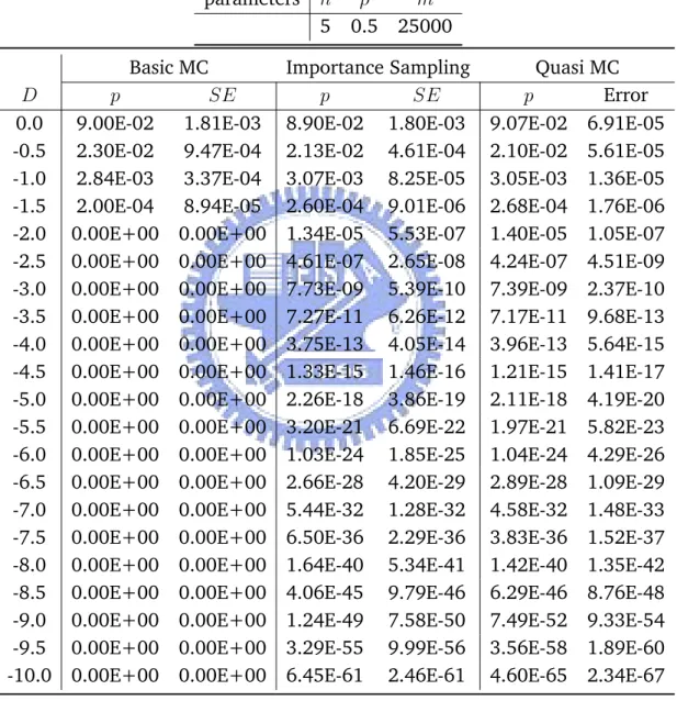
5.3 Numerical Comparison

We compare the performance of Basic MC, Importance Sampling and Quasi MC under different scenarios for Gaussian copula and Stuent-T copula. First we take into consideration the rarity of the default event by testing different threshold D. Recall that D = [d1, ..., dn]T = [Φ−1(F1(T )), ..., Φ−1(Fn(T ))]T. But

for simplicity, we let d1, ..., dn be equal to one constant and call it D. For our

purpose, we just need to test performance as D decreases, causing default to

be more rare so we do not need to construct D from Φ(.) and Fi(.) at the

moment. Then we compare performance of different methods with different number of firms, n. For constructing covariance matrix Σ we use the factor copula model and assume ρ1, ..., ρn are all equal and call it ρ.

In the following Tables,

• D = default threshold for each firm.

• df = degree of freedom for chi-square variable under Student-T copula • m = number of iterations in Basic Monte Carlo and Importance

Sam-pling method for Gaussian copula.

• m1 = number of iterations in evaluating inner expectation under

Condi-tional Importance Sampling for Student-T copula.

• m2 = number of iterations in evaluating outer expectation under

Condi-tional Importance Sampling for Student-T copula.

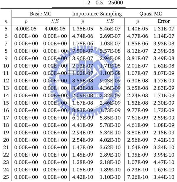
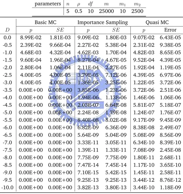
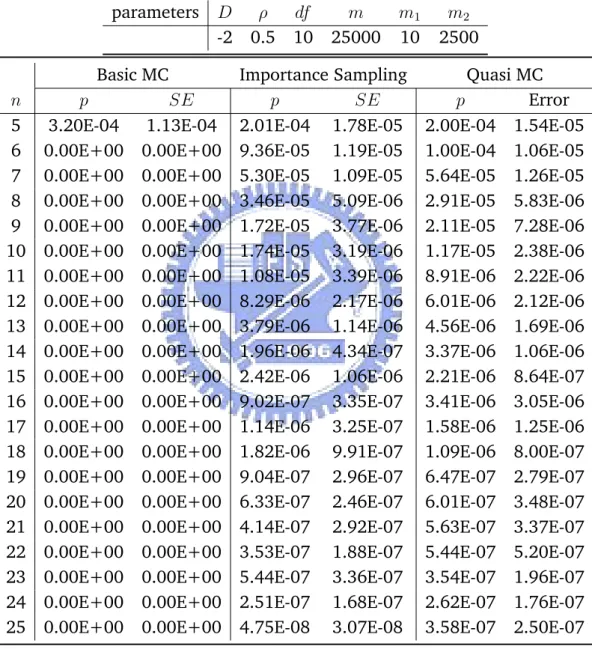
Under both Gaussian and Student-T copula, we can see importance sam-pling and Quasi MC both performed significantly better than Basic MC method. As D gets smaller, Basic MC method is no longer capable of sampling from such rare events. Importance sampling and Quasi MC are comparable in terms of performance when D gets very small and when n increases. Quasi MC seems more accurate overall, but importance sampling is a simpler, eas-ily modifiable and versatile approach. Given that the importance sampling method performs reasonably well under both Gaussian and Student-T copula, we take advantage of it’s simplicity and later apply it to more complex prob-lems such as calculating tail probability for some order statistics of default time, where Quasi MC method is not easily applicable.

Table 5.1: Estimating Joint Default Probability with Different Default Thresh-old under Gaussian Copula

parameters n ρ m

5 0.5 25000

Basic MC Importance Sampling Quasi MC

D p SE p SE p Error

0.0 9.00E-02 1.81E-03 8.90E-02 1.80E-03 9.07E-02 6.91E-05

-0.5 2.30E-02 9.47E-04 2.13E-02 4.61E-04 2.10E-02 5.61E-05

-1.0 2.84E-03 3.37E-04 3.07E-03 8.25E-05 3.05E-03 1.36E-05

-1.5 2.00E-04 8.94E-05 2.60E-04 9.01E-06 2.68E-04 1.76E-06

-2.0 0.00E+00 0.00E+00 1.34E-05 5.53E-07 1.40E-05 1.05E-07

-2.5 0.00E+00 0.00E+00 4.61E-07 2.65E-08 4.24E-07 4.51E-09

-3.0 0.00E+00 0.00E+00 7.73E-09 5.39E-10 7.39E-09 2.37E-10

-3.5 0.00E+00 0.00E+00 7.27E-11 6.26E-12 7.17E-11 9.68E-13

-4.0 0.00E+00 0.00E+00 3.75E-13 4.05E-14 3.96E-13 5.64E-15

-4.5 0.00E+00 0.00E+00 1.33E-15 1.46E-16 1.21E-15 1.41E-17

-5.0 0.00E+00 0.00E+00 2.26E-18 3.86E-19 2.11E-18 4.19E-20

-5.5 0.00E+00 0.00E+00 3.20E-21 6.69E-22 1.97E-21 5.82E-23

-6.0 0.00E+00 0.00E+00 1.03E-24 1.85E-25 1.04E-24 4.29E-26

-6.5 0.00E+00 0.00E+00 2.66E-28 4.20E-29 2.89E-28 1.09E-29

-7.0 0.00E+00 0.00E+00 5.44E-32 1.28E-32 4.58E-32 1.48E-33

-7.5 0.00E+00 0.00E+00 6.50E-36 2.29E-36 3.83E-36 1.52E-37

-8.0 0.00E+00 0.00E+00 1.64E-40 5.34E-41 1.42E-40 1.35E-42

-8.5 0.00E+00 0.00E+00 4.06E-45 9.79E-46 6.29E-46 8.76E-48

-9.0 0.00E+00 0.00E+00 1.24E-49 7.58E-50 7.49E-52 9.33E-54

-9.5 0.00E+00 0.00E+00 3.29E-55 9.99E-56 3.56E-58 1.89E-60

Table 5.2: Estimating Joint Default Probability with Different Number of Firms under Gaussian Copula

parameters D ρ m

-2 0.5 25000

Basic MC Importance Sampling Quasi MC

n p SE p SE p Error

5 4.00E-05 4.00E-05 1.35E-05 5.46E-07 1.40E-05 1.31E-07

6 0.00E+00 0.00E+00 4.74E-06 2.69E-07 4.77E-06 1.14E-07

7 0.00E+00 0.00E+00 1.78E-06 1.03E-07 1.85E-06 3.93E-08

8 0.00E+00 0.00E+00 7.50E-07 5.57E-08 8.12E-07 2.39E-08

9 0.00E+00 0.00E+00 3.96E-07 2.94E-08 3.81E-07 3.49E-08

10 0.00E+00 0.00E+00 2.13E-07 1.71E-08 2.01E-07 1.62E-08

11 0.00E+00 0.00E+00 1.02E-07 1.10E-08 1.07E-07 8.07E-09

12 0.00E+00 0.00E+00 8.55E-08 9.43E-09 6.30E-08 4.77E-09

13 0.00E+00 0.00E+00 3.43E-08 4.36E-09 3.65E-08 2.83E-09

14 0.00E+00 0.00E+00 2.09E-08 2.32E-09 2.24E-08 1.71E-09

15 0.00E+00 0.00E+00 1.67E-08 2.46E-09 1.52E-08 2.30E-09

16 0.00E+00 0.00E+00 8.83E-09 1.73E-09 9.77E-09 1.73E-09

17 0.00E+00 0.00E+00 6.17E-09 8.85E-10 7.61E-09 2.59E-09

18 0.00E+00 0.00E+00 4.41E-09 5.78E-10 4.61E-09 1.08E-09

19 0.00E+00 0.00E+00 2.94E-09 5.34E-10 3.80E-09 2.15E-09

20 0.00E+00 0.00E+00 2.54E-09 4.02E-10 2.56E-09 7.42E-10

21 0.00E+00 0.00E+00 1.47E-09 3.62E-10 1.64E-09 3.34E-10

22 0.00E+00 0.00E+00 1.45E-09 2.89E-10 1.35E-09 3.99E-10

23 0.00E+00 0.00E+00 1.28E-09 2.18E-10 1.07E-09 4.47E-10

24 0.00E+00 0.00E+00 1.05E-09 1.89E-10 6.23E-10 1.67E-10

Table 5.3: Estimating Joint Default Probability with Different Default Thresh-old under Student-T Copula

parameters n ρ df m m1 m2

5 0.5 10 25000 10 2500

Basic MC Importance Sampling Quasi MC

D p SE p SE p Error

0.0 8.99E-02 1.81E-03 9.09E-02 1.80E-03 9.07E-02 6.43E-05

-0.5 2.39E-02 9.66E-04 2.27E-02 5.38E-04 2.31E-02 9.38E-05

-1.0 4.68E-03 4.32E-04 4.62E-03 1.70E-04 4.82E-03 8.65E-05

-1.5 9.60E-04 1.96E-04 8.27E-04 4.67E-05 9.52E-04 4.39E-05

-2.0 2.80E-04 1.06E-04 2.11E-04 2.27E-05 1.92E-04 1.19E-05

-2.5 4.00E-05 4.00E-05 3.79E-05 7.12E-06 4.39E-05 6.97E-06

-3.0 4.00E-05 4.00E-05 1.36E-05 3.25E-06 1.22E-05 3.72E-06

-3.5 0.00E+00 0.00E+00 3.85E-06 1.23E-06 3.72E-06 2.51E-06

-4.0 0.00E+00 0.00E+00 1.94E-06 1.13E-06 1.46E-06 1.06E-06

-4.5 0.00E+00 0.00E+00 2.03E-07 6.64E-08 5.81E-07 5.18E-07

-5.0 0.00E+00 0.00E+00 2.24E-08 1.79E-08 1.24E-07 1.76E-07

-5.5 0.00E+00 0.00E+00 8.40E-08 8.02E-08 9.17E-09 9.45E-09

-6.0 0.00E+00 0.00E+00 6.82E-09 6.36E-09 8.38E-08 2.49E-07

-6.5 0.00E+00 0.00E+00 5.64E-09 5.04E-09 5.08E-09 8.56E-09

-7.0 0.00E+00 0.00E+00 3.33E-11 3.05E-11 6.34E-10 8.39E-10

-7.5 0.00E+00 0.00E+00 1.39E-11 1.33E-11 7.08E-09 2.45E-08

-8.0 0.00E+00 0.00E+00 7.75E-09 7.75E-09 1.80E-11 2.68E-11

-8.5 0.00E+00 0.00E+00 7.47E-14 7.45E-14 1.17E-10 3.65E-10

-9.0 0.00E+00 0.00E+00 7.10E-15 5.42E-15 1.45E-11 2.58E-11

-9.5 0.00E+00 0.00E+00 9.25E-13 9.25E-13 3.44E-12 8.76E-12

Table 5.4: Estimating Joint Default Probability with Different Number of Firms under Student-T Copula

parameters D ρ df m m1 m2

-2 0.5 10 25000 10 2500

Basic MC Importance Sampling Quasi MC

n p SE p SE p Error

5 3.20E-04 1.13E-04 2.01E-04 1.78E-05 2.00E-04 1.54E-05

6 0.00E+00 0.00E+00 9.36E-05 1.19E-05 1.00E-04 1.06E-05

7 0.00E+00 0.00E+00 5.30E-05 1.09E-05 5.64E-05 1.26E-05

8 0.00E+00 0.00E+00 3.46E-05 5.09E-06 2.91E-05 5.83E-06

9 0.00E+00 0.00E+00 1.72E-05 3.77E-06 2.11E-05 7.28E-06

10 0.00E+00 0.00E+00 1.74E-05 3.19E-06 1.17E-05 2.38E-06

11 0.00E+00 0.00E+00 1.08E-05 3.39E-06 8.91E-06 2.22E-06

12 0.00E+00 0.00E+00 8.29E-06 2.17E-06 6.01E-06 2.12E-06

13 0.00E+00 0.00E+00 3.79E-06 1.14E-06 4.56E-06 1.69E-06

14 0.00E+00 0.00E+00 1.96E-06 4.34E-07 3.37E-06 1.06E-06

15 0.00E+00 0.00E+00 2.42E-06 1.06E-06 2.21E-06 8.64E-07

16 0.00E+00 0.00E+00 9.02E-07 3.35E-07 3.41E-06 3.05E-06

17 0.00E+00 0.00E+00 1.14E-06 3.25E-07 1.58E-06 1.25E-06

18 0.00E+00 0.00E+00 1.82E-06 9.91E-07 1.09E-06 8.00E-07

19 0.00E+00 0.00E+00 9.04E-07 2.96E-07 6.47E-07 2.79E-07

20 0.00E+00 0.00E+00 6.33E-07 2.46E-07 6.01E-07 3.48E-07

21 0.00E+00 0.00E+00 4.14E-07 2.92E-07 5.63E-07 3.37E-07

22 0.00E+00 0.00E+00 3.53E-07 1.88E-07 5.44E-07 5.20E-07

23 0.00E+00 0.00E+00 5.44E-07 3.36E-07 3.54E-07 1.96E-07

24 0.00E+00 0.00E+00 2.51E-07 1.68E-07 2.62E-07 1.76E-07

Chapter 6

Application II: Basket Default

Swap

6.1 Introduction to Basket Default Swaps

We now wish to apply our importance sampling scheme in evaluating joint de-fault probability to evaluating multi-name credit derivatives. This is motivated by CYH’s study [5] on BDS. CYH mainly employed conditional importance sampling under the Gaussian copula factor model. We will first correct his ap-proach which seems to only consider the outer expectation. Then we suggest a different conditional importance sampling scheme which improves accuracy under specified conditions. In this case, we perform change of measure as suggest by results in Section 4.3. Finally, we introduce direct importance sam-pling based on the method used in evaluating joint default probability. Lastly, we will compare performance of these methods under Gaussian copula model. As an extension, we apply similar method to evaluating BDS under Student-T copula and compare it with Basic MC.

The mechanism of a credit default swap (CDS) is similar to that of an insur-ance. The protection buyer makes periodical premium payments (protection leg or PL) until some credit events happen. Then swap issuer compensates for the non-recovered part of the reference entities’ notional amounts (de-fault leg or DL). CDS provides credit protection only for a single underlying. Multi-name credit derivatives, such as BDS and CDO have gained increasing popularity in recent years because they extend credit protection to a pool of underlying. We focus on BDS in this study which provides protection to a