捲積管制圖之設計 - 政大學術集成

全文

(1)國立政治大學統計學系碩士學位論文. 指導教授：楊素芬博士. 捲積管制圖之設計. The Design of the Convolution Chart. 研究生：鄭鈞遠中華民國一百年六月.

(2) 國立政治大學統計學系碩士學位論文. 指導教授：楊素芬博士. 政治大. 立捲積管制圖之設計. ‧ 國. 學. The Design of the Convolution Chart ‧. n. er. io. sit. y. Nat. al. Ch. engchi. i Un. v. 研究生：鄭鈞遠中華民國一百年六月.

(3) 謝辭本篇論文的完成得力於諸多人士的幫忙。在此，獻上我的感謝之意。. 首先，感謝我的指導教授楊素芬老師，對於他的指導、支持、以及在整個過程中耐心的付出。此外，楊老師教導我做人處事的道理更是彌足珍貴的經驗。另外，感謝鄭惟孝老師以及葉小蓁老師提供的建議，讓我能更順利的完成論文，沒有兩位老師，整個過程會更加的艱辛。. 立. 政治大. 感謝我的同班同學，給了我如此精彩的兩年，特別是呂雨築、歐家玲、與謝. ‧ 國. 學. 志芬。有妳們陪伴的時光是這生難以忘懷的記憶。. ‧. 最後，感謝我的家人，他們在這段期間的精神支持與鼓勵是我不可或缺的動. n. al. er. io. sit. y. Nat. 力。. Ch. i Un. v. 本論文承蒙行政院國家科學委員會補助，計畫編號 NSC 98-2118-M-004-. engchi. 005-MY2，以及政治大學商學院 research team 補助，特此感謝。. 鄭鈞遠謹致中華民國100年六月. II.

(4) 立. 政治大. ‧. ‧ 國. 學. n. er. io. sit. y. Nat. al. Ch. engchi. III. i Un. v.

(5) Table of Contents Chapter 1. Introduction……………………………………...………………...…….1 1.1 Controlling High Yield Manufacturing Processes………………………...…….1 1.2 Motivation and Objectives…………………………………………………..….2 1.3 Literature Review……………………………………………………………….3 Chapter 2. Performance Comparison Among the C Chart, CQC Chart, Transformed EWMA Chart and CQC EWMA Chart………………10 2.1 Control Limits of Cumulative Quantity Control Chart, Transformed EWMA. 政治大 2.2 An Example of the Cumulative Quantity Control Charts, Cumulative Quantity 立. Chart and Cumulative Quantity Control EWMA Chart….……………………10. ‧ 國. 學. Control EWMA and Transformed EWMA Chart……………………………...12 2.3 Average Run Length Analysis…………………………………………………15. ‧. Chapter 3. The Design of the Convolution EWMA Chart with Normal. Nat. sit. y. Measurement Error…………………………………………………....18. n. al. er. io. 3.1 Measurement Error with Normal Distribution…………………………..…….18. i Un. v. 3.2 Design of the Exponential - Normal EWMA Convolution Chart……………..21. Ch. engchi. 3.3 Average Run Length of the Chart………………………………………..…….21 3.4 Average Run Length Calculation………………………………………….......23 3.5 The Impact of the Mistaking of the Chart……………………………….…….47 Chapter 4. The Design of the EWMA Convolution Chart with Exponential Measurement Error……………………………………………….......51 4.1 Measurement Error with Exponential Distribution…………………..………..51 4.2 Design of the Exponential - Exponential EWMA Convolution Chart…..…….52 4.3 Average Run Length of the Exponential-Exponential EWMA Convolution Chart …………………………………………………………………………..53. IV.

(6) 4.4 The Impact of the Mistaking of the Chart……………………………………..77 Chapter 5. Conclusion and Future Researches…………………...………………83 Reference…………………………………………………………………………….85. 立. 政治大. ‧. ‧ 國. 學. n. er. io. sit. y. Nat. al. Ch. engchi. V. i Un. v.

(7) List of Tables Table 1.. Observed Time Between Failures of a Capacitor……………..….……….12. Table 2. ARLs of CQC and EWMA CQC Charts………………………….….…...17 Table 3. ARLs under Different values of  , L1 and L2………………….………...24 Table 4. The ARL under the combination of  with   0.05 and ( L1 , L2 )  (3,2.072 ) and  2.  1.. ………………………………………………….…….….…...28. Table 5. The ARL under the combination of  with   0.1 , ( L1 , L2 )  (3.5,2.055) and  2  1 …………………………………………………….……………......29. 政治大 ………………………………………………….…….……………..30 立. Table 6. The ARL under the combination of  with   0.2 , ( L1 , L2 )  (4,1.925) and  2 1. ( L1 , L2 )  (4.5,1.756). ‧ 國. 學. Table.7 The ARL under the combination of  with   0.3 ,. and.  2  1 ……………………………………………….……….…...………..31. ‧. Table 8. The ARL under the combination of  with   0.4 ,. ( L1 , L2 )  (5,1.6057 ). and. sit. y. Nat.  2  1 …………………………………………….………………..……...32. n. al. ( L1 , L2 )  (5.5,1.4743). and. er. io. Table 9. The ARL under the combination of  with   0.5 ,. i Un. v.  2  1 …………………………………………..…...……………………...33. Ch. engchi. Table 10. The ARL under the combination of  with   0.05 , ( L1 , L2 )  (3,2.072 ) ,  2  1 ,   1000000. ……………………………...………………………….34. Table 11. All reasonable combinations of  , L1 and L2 for the Exponential-Normal EWMA convolution chart. (under  2  1 ,   100 )…………..…………35 Table 12. L2 values under different combination of  and L1 with different size of the  2 /  2 ratio for   100 ……………...………………………...…...36 Table 13. ARLs under different combinations of  , L1 and L2 with  2 /  2  0.0001 ,   100 ………………………………..…………………………………...38. Table 14. ARLs under different combinations of  , L1 and L2 with  2 /  2  0.1 ,. VI.

(8)   100 …………………………………..………………………………...40. Table 15. ARLs under different combinations of  , L1 and L2 with  2 /  2  0.25 ,   100 …………………...…………...…………………………………...42. Table 16. ARLs under different combinations of  , L1 and L2 with  2 /  2  0.5 ,   100 …………………………………………………………..…….…...44. Table 17. The impact of various values of  2 /  2 , L1 and L2 with   0.05 on ARLs……….……………………………………………………………46 Table 18. ARLs under different  2 /  2 , L1, L2,  between the Exponential-Normal EWMA convolution chart and misusing. 治政 Normal-Normal EWMA chart……………………………………..…......49 大立 Table 19. ARLs under different combination of , L and L by assuming . 1. 2. ‧ 國. 學. U  X   2 , X ~ EXP (   100 ) ,  2 ~ EXP(  1) …………………………...55. ‧. Table 20. The ARLs under the combination of  with   0.05 , ( L1 , L2 )  (3, 2.072) ,. io. y. sit. The ARLs under the combination of  with   0.1 , ( L1 , L2 )  (3.5, 2.055) ,. er. Table 21.. Nat.  2  1 ………………………………………………………...………….....59.  2  1 ……………………………..………………………………..………60. al. n. iv n C The ARLs under the combination U   0.2 , h e n g cofhi with. Table 22.. ( L1 , L2 )  ( 4,1.925) ,.  2  1 ……………………………………………………………………….61. Table 23. The ARLs under the combination of  with   0.3 , ( L1 , L2 )  (4.5,1.7561) ,  2  1 ………………………………………………….……………………62. Table 24. The ARLs under the combination of   0.4 , ( L1 , L2 )  (5,1.6057 ) ,  2  1 …………………………………………………………………......63. Table 25. The ARLs under the combination of   0.5 , ( L1 , L2 )  (5.5,1.4744 ) ,  2  1 …………………………………………………………..……….....64. Table 26. The ARLs under the combination   0.05 , ( L1 , L2 )  (3, 2.072) ,  2.  1,.   1000000 ……………………………….…………………….………...65 VII.

(9) Table 27. All reasonable combinations of  、L1、L2 for the Exponential-Exponential EWMA convolution chart (  2.  1 ,   100 )……66. Table 28. L2 Values under different combination of  , L1 with different size of the  2 /  2 ratio (   100 )…...………………………………………….......67. Table 29. ARLs under different combination of  、L1、L2 with  2 /  2  0.0001 ,   100 …………………………………………………………………...68. Table 30. ARLs under different combination of  、L1、L2 with  2 /  2  0.1 ,   100 ……………………………………………………………....…...70. Table 31. ARLs under different combination of  、L1、L2 with  2 /  2  0.25 ,. 政治大.   100 …………………………………………………………………...72. 立. Table 32. ARLs under different combination of  、L1、L2 with  2 /  2  0.5 ,. ‧ 國. 學.   100 …………………………………………………………………...74. ‧. Table 33. The impact of various values of  2 /  2 on ARL……..………..………76. sit. y. Nat. Table 34. ARLs under different  2 /  2 、L1、L2 and  between the. io. er. Exponential-Exponential EWMA convolution chart and the mistaking of Normal-Normal EWMA chart (   0.05 )………………………………...79. al. n. iv n C ARLs under different h /  、L1、L2 and e n g c h i U  between the misused. Table 35.. 2. 2. Normal-Normal EWMA with parameter  and Normal-Normal EWMA with parameter  (   0.05 )…………………………………………...81. VIII.

(10) List of Figures Figure 1.. The CQC Chart………………………………………….……..…...……13. Figure 2.. The EWMA Transformed Chart…………………………………..……..14. Figure 3.. The EWMA CQC Chart………………………….……………..………..15. Figure 4.. The ARL under the combination of  with   0.05 ,. ( L1 , L2 )  (3,2.702 ). and.  2  1 .……………………………………………...………………………28. Figure 5.. The ARL under the combination of  with   0.1 ,. ( L1 , L2 )  (3.5,2.055). and.  2  1 ……………………………………………..……………………..…29. Figure 6.. 2. ‧ 國. The ARL under the combination of  with.   0.3 , ( L1 , L2 )  (4.5,1.7565 ). 學. Figure 7.. 政治大  1 ……………………………………………………………………...30 立. The ARL under the combination of  with   0.2 , ( L1 , L2 )  (4,1.925) and. and  2  1 ……………………………………………………………......31. ‧. Figure 8.. The ARL under the combination of  with   0.4 , ( L1 , L2 )  (5,1.6057 ) and. y. sit. n. al. er. The ARL under the combination of  with   0.5 , ( L1 , L2 )  (5.5,1.4743) ,. io. Figure 9.. Nat.  2  1 ………………………………………………………………….....32. i Un. v.  2  1 …………………………………………………………………......33. Figure 10.. Ch. engchi. The ARL under the combination of  with   0.05 , ( L1 , L2 )  (3,2.702 ) ,  2  1 and   1000000 ……..………………………….…………………34. Figure 11.. The ARLs under the combination of  with   0.05 , ( L1 , L2 )  (3, 2.072 ) ,  2  1……………………………………………………………………….59. Figure 12.. The ARLs under the combination of   0.1 , ( L1 , L2 )  (3.5, 2.055) ,  2  1 ……………………………………………………………………….60. Figure 13.. The ARLs under the combination of  with   0.2 , ( L1 , L2 )  (4,1.925) ,  2  1 ……………………………………………………………………….61. Figure 14.. The ARLs under the combination of   0.3 , ( L1 , L2 )  (4.5,1.7561) ,. VIII.

(11)  2  1 ……………………………………………………………..………….62. Figure 15.. The ARLs under the combination of  with   0.4 , ( L1 , L2 )  (5,1.6057 ) ,  2  1 ……………………………………………………………………….63. Figure 16.. The ARLs under the combination of   0.5 , ( L1 , L2 )  (5.5,1.4744 ) ,  2  1 …………………………………………………………………….....64. Figure 17. The ARLs under the combination   0.05 , ( L1 , L2 )  (3, 2.072 ) ,  2  1 ,   1000000 ………………... ………….…………………..….………..65. 立. 政治大. ‧. ‧ 國. 學. n. er. io. sit. y. Nat. al. Ch. engchi. VIII. i Un. v.

(12) Abstract Measurement error is an important factor in industry that influences the outcome of a process. Large measurement error would cause the observation measure deviate from the true value and consequently lead to a wrong decision. In this project, we propose a convolution control chart. We then design the EWMA ‗time between events‘ (TBE) control chart with the measurement error, with the assumption that the observations are exponentially distributed. In addition, we assumed the measurement error follows a normal distribution or an exponential distribution. We showed that, in two cases of. 治政 the measurement error, the performance of the proposed 大chart monitoring the process 立 mean is greatly affected. ‧. ‧ 國. 學. n. er. io. sit. y. Nat. al. Ch. engchi. VIII. i Un. v.

(13) Chapter 1. Introduction 1.1 Controlling High Yield Manufacturing Processes Many statistical process control (SPC) techniques have been proposed since 1920‘s when Walter Shewhart first introduced the control charts (Shewhart, 1924). After that, SPC charts were widely applied in improving the quality of manufacturing products. The main purpose in using any control chart is to monitor a process and to identify the causes of any unusual signals and rectify them to bring the process. 政治大. in-control. There are many control charts -- the traditional Shewhart charts like X-bar. 立. and R charts, c and u charts, CUSUM and EWMA charts.. ‧ 國. 學. These days, as the emphasis on the quality of products and customer satisfaction increased, the high yield process with very low parts per million (ppm) (Xie and Goh. ‧. 1992) defections of rare defects draw lots of attention from manufacturers and. y. Nat. io. sit. practitioners. It is important to monitor such processes properly. Unfortunately, the. n. al. er. traditional c and u charts may not perform well in high yield processes. When an. Ch. i Un. v. ordinary c chart is used for monitoring such processes, most measured values are all. engchi. zeroes since the defect rate is extremely low (unless we have a huge sample). Consequently, it is impossible to observe any non-conforming units with small samples and the monitoring action became useless. To overcome this difficulty in high yield environment, the ‗time between events‘ (TBE) control charts were introduced. These charts monitor the time between defects or the good units between consecutive defects instead of monitoring the number of defects in a given time interval. TBE chart could help solve the problem when using the traditional c and u charts in high yield processes (Xie et al. 2002). TBE chart is superior to the c and u charts and it can be implemented easily in automated 1.

(14) manufacturing processes. A widely accepted model for TBE data is the exponential distribution, like the ‗Cumulative Quantity Control‘ (CQC) chart (Chan et al. 2000), the exponential ‗Cumulative Sum‘ (CUSUM) chart (Lucas 1985, Vardeman and Ray 1985)、and the exponential EWMA chart (Gan 1998). Hawkins and Olwell (1998) studied the Weibull CUSUM chart. Among those charts, TBE ‗Exponentially Weighted Moving Average‘ (EWMA) chart is recommended since it could easily detect small shifts. So the CQC EWMA chart is a widely used SPC tool in TBE monitoring.. 1.2 Motivation and Objectives. 立. 政治大. Measurement error of a gauge is an important factor in industry that influences. ‧ 國. 學. the outcome of a process. When a process involved measurement, some of the. ‧. observed variability will be inherent in the items that are being measured. And the rest. sit. y. Nat. of the variability might come from the measurement system being used. Measurement. io. er. error could attribute its error to the gauge capability、environment、the operator and. al. other factors. Large measurement error will cause the observation measure deviate. n. iv n C from the true value and consequently to a wrong decision. Although we could h elead ngchi U. adjust the gauge to reduce the impact, however some measurement error will still exist nonetheless. Many studies would assume the process is measurement error free. This is against the reality. In view of this, we would like to introduce a new approach, i.e. an EWMA convolution control chart. We assume the measurement error follows a normal distribution or an exponential distribution. According to the relationship among the true value、the measurement error、and the observed value, we could derive the probability density function of the observed value via the convolution. Thus the new EWMA control 2.

(15) chart constructed by the observed value is called the ‗EWMA Convolution Chart‘. We examine the effect of measurement error on the power of the EWMA convolution chart to detect out-of-control situations by the ‗Average Run Length‘ (ARL). We will show that, in two cases of the measurement error, the performance of the EWMA convolution chart in monitoring the process is greatly affected. In chapter 2, we would show the shortcomings of the c chart. In chapter 3, we will introduce an EWMA Exponential–Normal convolution chart, and the EWMA Exponential–Exponential convolution chart in chapter 4. Both chapters also discuss the impact of the measurement error on the proposed charts. In chapter 5 we give the. 治政 conclusion and some potential future research projects.大立 ‧ 國. 學. 1.3 Literature Review. ‧. In 1924, Walter Shewhart first introduced the control charts (Shewhart, (1924)). io. er. charts for attributes data like p、c and u charts.. sit. y. Nat. and after that, some other control charts were proposed by many scholars. The control. al. (1). The Traditional P Chart. n. iv n C Supposed the probability of any conforming to specifications in a stable h eunitn not gchi U. process is p. To construct a p chart to monitor such a process, we take samples of fixed size n, and count the number of non-conforming units, D, then D follows a binomial distribution with n and p. The mean and variance of D are np and np(1-p) respectively. The sample fraction non-conforming is defined as the ratio of the number of non-conforming units in the sample, D, to the sample size n, that is, pˆ  D / n , the mean and variance of pˆ are p and p(1-p)/n respectively. Thus, the control limits of the p chart (see Montgomery (2009)) are：. UCL P  p  3. 3. p(1  p) n. (1).

(16) CL P  p. (2). LCL P  p  3. p(1  p) n. (3). UCL P  pˆ  3. pˆ (1  pˆ ) n. (4). with p known, or. CL P  pˆ. (5). pˆ (1  pˆ ) n. LCL P  pˆ  3. (6). with unknown p.. 政治大 we‘re unable to observe any non-conforming units since the defect rate is extremely 立 One major problem when we use p chart to monitoring the high yield process is,. ‧ 國. 學. low (unless we have a huge sample), thus the plotting points on the p chart are sequences of zeroes. The monitoring action is useless.. ‧. (2). The Traditional C Chart. sit. y. Nat. Suppose that the rate of occurrence of defects in a stable process is 1 / . al. er. io. defect(s) per unit quantity of product produced, that is, the expected number of. v. n. non-conformities during the given sampling interval is 1 /  . Here 1 /   0 is not. Ch. engchi. i Un. necessarily an integer. To construct a c chart to monitor such a process, we take samples of fixed size n, and record the number of defect, c, in each sample, calculate the average value c of the observed c‘s. Since the process has a stable defect rate 1 /  , c is a Poisson random variable with mean and variance both equal to n /  , that is, c ~ Poi (n /  ) . The control limits of the c chart (see Montgomery (2009)) are：. UCL C  c  3 c. (7). CLC  c. (8). LCLC  c  3 c. (9). 4.

(17) (3). The Traditional U Chart For manufacturing processes where products are produced continuously it is impractical to take the sample of the same size n each time, hence u chart should be used. If we find c total non-conformities in a sample of n inspection units, then the average number of non-conformities per inspection unit is u = c / n. The mean and the variance of u are. E (u )  1 /  and Var (u )  1 / n the control limits (see Montgomery (2009)) are：. UCLU  u  3. 政治大. (10). CLU  u. LCLU  u  3. (11). 學. ‧ 國. 立. u n. u n. (12). ‧. If u is not known then u is instead of u, where u represent the observed average. y. Nat. io. sit. number of non-conformities per unit in a preliminary set of data.. n. al. er. The main problem of the traditional c and u charts while monitoring the high. Ch. i Un. v. yield process is that we are unable to observe any non-conforming units since the. engchi. defect rate is extremely low (unless we have a huge sample), thus the plotting points on the c chart are sequences of zeroes. As consequence, the monitoring action became useless. (4). The EWMA chart The EWMA chart was first proposed by Roberts (1959) and commonly used for its superiority in detecting small process shifts. The idea behind this is that it accumulates current and past information from the observations and has been proven to be more effective than Shewhart-type charts in detecting small shifts in the process mean. 5.

(18) Borror, Champ and Rigdon (1998) showed the superiority of Poisson EWMA chart to the traditional c chart, due to its smaller out-of-control ARLs and the lower control limit is usually positive so the downward change on the process mean could be detected. (5) Geometric chart Glushkovsky (1994) studied the geometric chart, and compared it with the traditional p chart. The control limits of the geometric chart are：. UCLU  G ln( ). (13). 政治大. (14).  G ln(1   ). (15). CLU  G ln( 0.5). 立 LCL. U. ‧ 國. 學. where G is the average number of conforming units between two consecutive. ‧. appearances of non-conforming ones. The centre line is set at the median of G.. sit. y. Nat. The result showed that, geometric chart provides more dynamic, quicker. io. er. response than the p chart, due to the smaller out-of-control ARLs.. al. (6). Cumulative Count Control. n. iv n C Kuralmani, Xie, Goh and Ganh(2002) added a condition to the geometric chart, engchi U. or called Cumulative Count Control (CCC) chart to improve the sensitivity. The idea behind this is simply taking the previous run into consideration when the present point did not fall between the control limits. Thus, the process is in-control if (a) the count of the conforming units fell between the lower and upper control limits, or (b) the count of the conforming units fell outside the lower or upper control limits but the previous s runs were in-control. Their study showed that comparing to the CCC chart, the conditional chart would have tighter control limits under the same false alarm rate and smaller out-of-control ARLs under moderate to large process shifts. Also, to get larger in-control ARLs the false alarm rate should be reduced at the designed process 6.

(19) stage. (7). Cumulative Quantity Control However, the CCC chart is constructed based on a discrete distribution. In some situation, the quality measure is better illustrated by a continuous distribution, like the exponential distribution. Thus, a control chart constructed by the exponential distribution, called ‗Cumulative Quantity Control‘ (CQC) chart, which monitor the time between defects or the good units between consecutive defects instead of monitoring the number of defects in a time interval, were introduced by Chan, Xie and Goh (2000).. 治政 Chan, Xie and Goh (2000) showed the CQC chart 大is superior to the traditional c 立 and u charts. They also pointed out that the CQC chart doesn‘t have the shortcomings ‧ 國. 學. of the c and u charts - giving false alarm signals too frequently when the process. sit. y. Nat. dependent upon the sample size of each group.. ‧. defect rate is low or moderate. Additionally, the performance of the CQC chart is not. io. er. However, CQC chart has another problem, when process has slightly to. al. moderate deteriorates, its out-of-control ARL will be greater than its in-control ARL. n. iv n C value. It definitely not the situationhwe want, since the e n g c h i U early detection of the process deteriorates is always our primary concern. To deal with this, some scholars suggested. transform the exponential distribution to an approximately normal distribution by taking the ‗double square root transformation‘. (8). Transformed exponential chart Liu, Xie, Goh and Chan (2006) and Liu, Xie, Goh (2006) studied the transformed exponential chart. They transformed an exponential distribution to an approximate normal distribution by taking the ‗double square root transformation‘, then used the transformed data to construct a EWMA or CUSUM chart. The results showed that the proposed transformed EWMA or CUSUM chart is more effective 7.

(20) than the X-MR, CQC chart, especially when the process deteriorated. However, the EWMA transformed chart would have similar ARL values to the CQC EWMA chart. Also, it was comparable to the CQC CUSUM chart in detecting the process improvement or deterioration. One way to improve the sensitivity of the CQC chart is the CQC-r chart. The CQC-r chart was proposed to monitor the time until a specified number (r) of events observed based on gamma distribution. The CQC-r chart provides more credibility to the decision regarding the statistical control of the process as the decision is made on. 政治大 case of the CQC-r chart by setting r = 1. 立. the basis of r events rather than a single event. Indeed, the CQC chart is the special. ‧ 國. 學. (9). TBE chart. Liu, Xie, Goh and Sharma (2006) studied some exponential TBE charts like the. ‧. CQC chart and its extension CQC-r chart that monitor the quantity inspected until the. Nat. sit. y. occurrence of a specified number, r, of defects. The performance of CQC-r chart were. n. al. er. io. compared to exponential EWMA, exponential CUSUM and CQC charts. The. i Un. v. conclusions are (i) when the process improvement is small, the exponential EWMA. Ch. engchi. chart is slightly better than the exponential CUSUM chart, and both of them are better than the CQC and CQC-r charts. (ii) Among the lower-sided exponential TBE charts, the ‗average time to signal‘ (ATS) of exponential EWMA and exponential CUSUM charts are much better than the CQC and the CQC-r charts. The EWMA exponential chart is more sensitive to small deterioration, while the exponential CUSUM chart is suitable for large deterioration. For the CQC-r chart, the larger the value of r, the better the performance. (iii) Among the two-sided exponential TBE charts, the exponential CUSUM and the exponential EWMA charts outperform the CQC-r chart. For CQC-r chart. When the process improves, the parameter r does not influence the. 8.

(21) ATS performance to a large extent, and when the process deteriorates, the CQC-r chart with large value of r shows distinct superiority to the CQC chart. (iv) The superiority of the exponential EWMA and the exponential CUSUM charts in ATS is less significant when the in-control ATS decreases to 370, and thus it makes the CQC and CQC-r charts a better choice because of their simple design procedure and less requirement of process information. From the above review, we could see the superiority of the exponential EWMA chart. It is the most effective one since it could detect the small shift of the process quickly whether its mean is an upward or downward shift. In view of this, we would. 治政 study the impact of the measurement error on the exponential 大 EWMA chart. 立 ‧. ‧ 國. 學. n. er. io. sit. y. Nat. al. Ch. engchi. 9. i Un. v.

(22) Chapter 2. Performance Comparison Among the C Chart, CQC Chart, Transformed EWMA Chart and CQC EWMA Chart. 2.1 Control Limits of CQC Chart, Transformed EWMA Chart and CQC EWMA Chart Suppose that defects in a process occur according to a Poisson process with mean rate of occurrence of 1 /  . Different from the traditional C chart, the number. 政治大. of conforming unit(s) X (which is not necessarily an integer) required to observe. 立. exactly 1 defect follows an exponential distribution (Walpole et al. (1998, chapter. ‧ 國. 學. 6)), i.e. X ~ EXP(  ) , with probability density function (p.d.f.), cumulative distribution function (c.d.f.) and mean respectively：. . x F ( x)  1  exp( ). n. al. Ch. er. io. . E (x)  . engchi U. (16). y. Nat. . x exp( ). sit. 1. ‧. f ( x) . v ni. (17) (18). where   0 , stands for the average time to find one nonconforming. Larger  means better process quality. The process is in-control when   1 , and out-of-control when   1 . The control limits of CQC Chart is (see Chan, Xie, and Goh (2000)). . UCL    ln( ) 2. (19). CL    ln( 0.5). (20). LCL    ln(1 .  ) 2. (21). note that the center line of a CQC chart is set at the median of X and  is the false alarm rate or the probability that sample x falls outside UCL. 10.

(23) Nelson (1994) proposed an alternative method by taking exponential data to the 1/3.6 ( ≒ 0.25) power so that the transformed variable becomes approximately normal. Now taking 0.25 power to X then we get a new random variable E follows a normal distribution, i.e. E = X 0.25, E ~ N (0.9064  0.25,0.0647  0.5 ) . The control limits for the transformed CQC chart are UCL  0.9064  0.25  3 0.0647  0.5. (22). CL  0.9064  0.25. (23). LCL  0.9064  0.25  3 0.0647  0.5. (24). 政治大. Using the transformed variable, E, to construct an EWMA control chart, the. 立. 學. ‧ 國. transformed EWMA statistic (Liu, Xie, Goh and Chan (2006)) is. Zi  Ei  (1   )Zi 1 ,.   , [1 - (1 -  ) 2i ]  0.0647  2 (2   ) 2. ‧. note that E(Z i )  0.9064  , V (Z i )  0.0647  2. io. sit. y. Nat. the control limits of the new EWMA chart are：. n. er. UCL  E(Z i )  L1 V(Z i )  0.9064   L1 0.0647  2. al. Ch. (25). engchi. CL  0.9064 . i Un. v. LCL  E(Z i )  L2 V(Z i )  0.9064   L2 0.0647  2.  (2   ). (26) (27).  (2   ). (28). Since normal is a symmetric distribution, the control limit parameters can be set the same value, i.e. L1 = L2. Gan (1998) proposed CQC EWMA Chart. To define a CQC EWMA chart, the statistic is. Z i  X i  (1   )Zi1 ,. 11. (29).

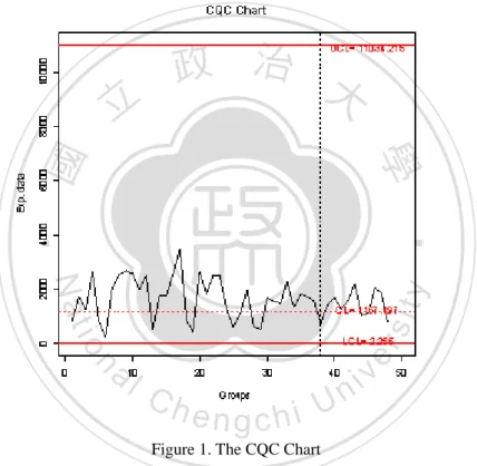
(24) note that E(Z i )   , V(Zi ) = b 2. l (2 - l ). [1-(1-l )2i ] = b 2. l 2-l. The control limits of the CQC EWMA chart are UCL  E(Z i )  L1 V(Z i )    L1  0. . 2. (2   ). CL  . (30) (31). LCL  E(Z i )  L2 V(Z i )    L2  2.  (2   ). (32). Since exponential is an asymmetric distribution, we set L1 ≠ L2 in the control limits.. 政治大 2.2 An Example of the CQC 立Charts, CQC EWMA and Transformed EWMA. ‧ 國. 學. Chart. In this section, we will use an example to compare the performance of the. ‧. three charts.. The following 48 measurements from Chan, Xie, and Goh (2000) are the. y. Nat. io. sit. observed times (in hours) between failures of a capacitor in an electricity supply. n. al. er. plant which is running in a stable condition. The data are arranged in the order of occurrence of the failures.. Ch. engchi. i Un. v. Table 1. Observed Time Between Failures of a Capacitor. 1-6 7-12 13-18 19-24 25-30 31-36 37-42 43-48. 836.90 2050.50 500.50 445.64 600.10 1555.12 1567.01 2234.49. 1760.00 2540.40 1780.00 2659.40 1102.58 1506.26 742.21 1053.49. 1250.50 2684.00 1759.00 1850.30 2003.15 2321.80 1469.79 1123.24. 2639.50 2608.40 2590.60 2520.50 644.99 1352.03 1713.03 2064.88. 867.40 1993.70 3502.80 2500.50 525.40 1852.55 1275.16 1860.57. 262.53 2530.70 860.40 1260.60 1688.20 1740.60 1586.53 745.63. We use the first 38 data to construct the control chart and the 39th to the 48th are. 12.

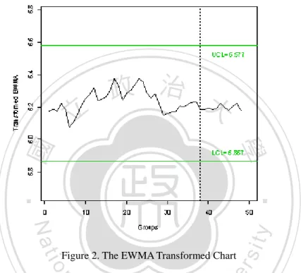
(25) the monitoring data. The average of these 38 values is ˆ  1669 .915 . (1). The CQC chart The control limits of the CQC chart are. . UCL   ˆ ln( )  1669 .915 ln(1  2 LCL   ˆ ln(1 . . 0.0027 )  11034 .215 2. )  1669 .915 ln(1 . 2. 0.0027 )  2.258 2. we plot the CQC chart, the result is shown in Figure 1.. 政治大. 立. ‧. ‧ 國. 學. n. er. io. sit. y. Nat. al. Ch. engchi. i Un. v. Figure 1. The CQC Chart. The CQC charts showed that the process is in-control since there are no points falling outside the control limits. (2). The transformed EWMA chart The factors ( L1 , L2 )  (2.508, 2.508 ) is determined by using the Markov chain approach in Lucas and Saccassuci (1990) to let ARL0 = 370, under   0.05 . The control limits of the transformed EWMA chart are：. 13.

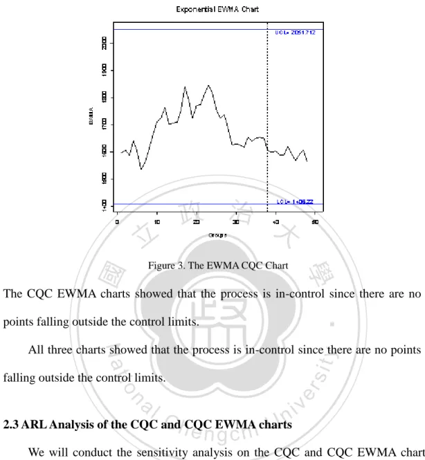
(26) . UCL  0.9064(1669.915)  2.508 0.0647 (1669.915) 2. LCL  0.9064 (1669 .915)  2.508 0.0647 (1669 .915)2.  6.577. (2   ).  (2   ).  5.887. We plot the transformed EWMA chart, the result is shown in Figure 2.. 立. 政治大. n. er. io. al. sit. y. ‧. ‧ 國. 學. Nat. Figure 2. The EWMA Transformed Chart. i Un. v. The transformed EWMA charts showed that the process is in-control since there are. Ch. engchi. no points falling outside the control limits.. (3). The CQC EWMA chart The factors ( L1 , L2 )  (3,2.072) is determined by using the Markov chain approach in Lucas and Saccassuci (1990) to let ARL0 = 370, under   0.05 . The control limits of the CQC EWMA chart are UCL  1669 .915  3 1669 .915. 0.05  2051 .712 2  0.05. LCL  1669 .915  2.072 1669 .915. 14. 0.05  1406 .22 2  0.05.

(27) We plot the CQC EWMA chart, the result is shown in Figure 3.. 立. 政治大. ‧ 國. 學. Figure 3. The EWMA CQC Chart. The CQC EWMA charts showed that the process is in-control since there are no. ‧. points falling outside the control limits.. Nat. sit. y. All three charts showed that the process is in-control since there are no points. er. io. falling outside the control limits.. n. al. ni C hCQC EWMA charts 2.3 ARL Analysis of the CQC and U engchi. v. We will conduct the sensitivity analysis on the CQC and CQC EWMA charts, with   100 . For the EWMA chart, we set   0.05 、 ( L1 , L2 )  (3, 2.072 ) . The ARLs of the control charts is calculate by using Markov Chain approach in Lucas and Saccassuci (1990). The last column in the Table 2, ‗ARL saved %‘ means the percentage saved by the CQC EWMA chart compared with the CQC chart, it can be expressed as：. ARL saved % . ARLCQC  ARLEW MA. 15. ARLCQC. (33).

(28) In addition, since the performance of the transformed EWMA chart is almost the same as the CQC EWMA chart (see Liu, Xie, Goh and Chan (2006)), so we just calculate and compare the ARLs of CQC and CQC EWMA charts, see Table 2.. 立. 政治大. ‧. ‧ 國. 學. n. er. io. sit. y. Nat. al. Ch. engchi. 16. i Un. v.

(29) Table 2.. ARLs of CQC and CQC EWMA Charts. . CQC. CQC EWMA. ARL saved %. 0.1. 1.936. 1.009. 47.88%. 0.2. 3.745. 1.191. 68.20%. 0.3. 7.238. 1.679. 76.80%. 0.4. 13.950. 2.702. 80.63%. 0.5. 26.725. 4.924. 81.58%. 0.6. 50.541. 10.215. 79.79%. 0.7. 93.063. 24.094. 74.11%. 0.8. 162.827. 63.985. 60.70%. 0.9. 261.161. 184.558. 29.33%. 1.0. 370.370. 370.605. -. 1.1. 458.271. 治 505.086 政 101.966 大 515.302 53.141 立. 50.32%. 503.643. 32.118. 93.62%. 1.5. 482.179. 21.639. 1.6. 457.720. 15.777. 96.55%. 1.7. 433.436. 12.196. 97.19%. 1.8. 410.590. 9.852. 97.60%. 389.564. 8.233. 97.89%. 370.370. 7.065. 352.879. 6.191. y. ‧ 國. 95.51%. ‧. 2.1. io. 2.0. Nat. 1.9. 學. 1.4. 89.69%. sit. 1.3. 79.81%. 98.09%. er. 1.2. 227.660. 98.25%. 2.4. 308.922. 4.561. 98.52%. 2.5. 296.591. 4.211. 98.58%. 2.6. 285.205. 3.920. 98.63%. 2.7. 274.662. 3.674. 98.66%. 2.8. 264.871. 3.464. 98.69%. 2.9. 255.755. 3.283. 98.72%. 3.0. 247.247. 3.126. 98.74%. 2.2. n. 2.3. al 336.918 Ch 322.318. n U i e n g4.989 h c 5.519. i v 98.36% 98.45%. From Table 2, we could see the superiority of the CQC EWMA chart, its ARL1 , i.e. when   1 , is always smaller than the CQC chart and the saved % of ARLs is substantial. This means the EWMA chart is more effective. 17.

(30) Chapter 3. The Design of the Convolution EWMA Chart with Normal Measurement Error. Nowadays, as product quality is of primary concern, manufacturers are pursuing for excellence. In high yield processes, the defect rate could be as low as several parts per million (ppm) (Xie and Goh 1992). Some charting procedures for monitoring such processes were studied by numerous authors, like Calvin (1983), Lucas (1989), Lawson and Hathway (1990), Goh (1991), Nelson (1994), Wheeler (1995), and others.. 治政 One of the charts is the CQC chart. The CQC chart has 大been shown to be very useful 立 for monitoring the high yield processes. However, in previous study, the assumption ‧ 國. 學. of 100% error free measurement was made. Some authors studied the measurement. ‧. error on Shewhart control charts, (see Linna and Woodall (2001) and Maravelakis,. sit. y. Nat. Panaretos and Psarakis (2004)), but none of them focus on the CQC chart.. io. er. Measurement error could attribute to the gauge capability, environment, the operator. al. and so on. Large measurement error would influence the observation deviating from. n. iv n C the true value and consequently leads chart to a wrong decision. The h e ntheg control chi U impacts of the measurement error on control charts have been discussed in Ryan (1989), Johnson et al. (1991), Burke et al. (1995) and Yang et al (2007). Although we can adjust the gauge to make the impact less, some measurement errors still exist while the units are being measured. In view of this, we consider the measurement error by assuming the error term follows a normal distribution or an exponential distribution. The convolution charts are thus constructed.. 3.1 Measurement Error with Normal Distribution Suppose that the number of defects occurred in a process follows a Poisson 18.

(31) distribution with mean rate of occurrence equals to 1 /  . Then the number of unit(s), X (which is not necessarily an integer), required to observe exactly 1 defect is an exponential random variable (Walpole et al. (1998, chapter 6)), i.e. X ~ EXP(  ) , the p.d.f., c.d.f. and mean of X are respectively：. x exp( ). (34). x F ( x)  1  exp( ). (35). E (x)  . (36). f ( x) . 1. . . . where   0 , stands for the average time to find one nonconforming, large . 政治大. means better process quality. The process is in-control when   1 , otherwise. 立. out-of-control.. ‧ 國. 學. Next, we add the measurement error into the consideration. As we had discussed above, as long as measurement error exists, the observed value will deviate from the. ‧. true value. Assume the true value of the product, X, is exponentially distributed,  1. sit. y. Nat. io. er. is the measurement error that follows a normal distribution. In this case, the. al. measurement error can be positive or negative, which means it can cause the observed. n. iv n C value greater or smaller than the true This measurement error comes from the h evalue. ngchi U equipment which is counting the number of conforming units to observe one non-conforming. Let the observed value be Y, the sum of X and  1 , i.e.：. Y  X  1. (37). where X and  1 are independent, and：.  1 ~ N (0, 2 ). (38). Using the convolution of normal distribution and exponential distribution, the p.d.f. of Y is：. 19.

(32)  2  y   y 2   1  f ( y)  exp   2     2     .      . (39). Proof： If Y  X   1 , set  1  t , then we can get x  y  t , by convolution y. f ( y )   f x ( y  t ) f 1 (t )dt .  t2   1  1 1 exp  ( y  t )  exp  2 dt      2 2  2 . . y. 政治大. t  y  y 1 1 t2    exp  ( )  exp  2 dt      2 2   2 . 立. ‧ 國. 學.  y  y 1 1 1  2 2 2  1 2 exp  ( )  exp[ 2  t 2  t  ( ) 2 ]dt exp[ 2 ( ) 2 ]      2 2  B  2  2 . n. sit.    C h engchi  . er. io.  2  y  aBl  y 2   1    exp   2     2     . ‧. Nat.  y 1 1 2 2 y 1 1  2     exp  ( )  2 ( )  exp[ 2  t  ]dt    2    2 2   2 . y. . i Un. v. #. From the relationship among X、  1 and Y, we could derive the mean and variance of Y. E (Y )  E ( X   1 )  E ( X )  E ( 1 )    0  . (40). V (Y )  V ( X   1 )  V ( X )  V ( 1 )  2 cov( X ,  1 )   2  0   2. (41). In fact, Y follows a special distribution called Ex-Gaussian (Luce (1986, chap. 6)), which is the sum of an exponential distribution and a normal distribution.. 20.

(33) 3.2 Design of the Exponential – Normal EWMA Convolution Chart Monitoring the Ex-Gaussian random variable by applying the EWMA chart, the Exponential–Normal EWMA convolution chart, when the process is in-control,   1 , the plotting statistic is. Z i  Yi  (1   )Z i 1. (42). E(Z i )  E(Y )  . (43). with mean and variance. V(Zi ) = V(Y ). l l l [1- (1- l )2i ] = (b 2 + s 2 ) [1- (1- l )2i ] » (b 2 + s 2 ) (44) 2-l 2-l 2-l. Z0 = E(Y ) = b. 學. ‧ 國. 治政 respectively. Assume the initial value of the EWMA 大statistics equals to the mean 立 value of Y, that is. (45). ‧. the control limits for the Exponential–Normal EWMA convolution chart is. y. Nat. n. al. Ch. CL  . engchi U. . 2. er. io. sit. UCL  E ( Z i )  L1 V ( Z i )    L1 (  2   2 ). v ni. LCL  E ( Z i )  L2 V ( Z i )    L2 (  2   2 ). (46) (47).  2. (48). Since Ex-Gaussian is not a symmetric distribution, the control limit parameter, L1 and L2 needn‘t be set the same value.. 3.3 Average Run Length of the Exponential – Normal EWMA Convolution Chart The Average Run Length (ARL) is used to measure the performance of a control chart. ARL is the average number of samples taken before finding an out-of-control signal. The Markov Chain approach was first introduced by Brooks and Evans (1972).. 21.

(34) This approach could be applied to find ARL when we couldn‘t find it by solving expressive equations. We divide the interval ( LCL , UCL ) into N small subintervals (Lucas and Saccucci (1990)), the jth subinterval is denoted by ( L j ,U j ) , where. L j  LCL . ( j  1)(UCL  LCL ) N. (49). ( j )(UCL  LCL ) N. (50). (2 j  1)(UCL  LCL ) 2N. (51). U j  LCL  The jth subinterval‘s midpoint, m j is. m j  LCL . 政治大. The (N+1)th state in which the point is not within the control limits, either greater. 立. than the upper limit or smaller than the lower limit, is designated as the absorbing. ‧ 國. 學. state. The transition probability Pij is the probability that given the state of statistic Z. y. (52). sit. Nat. Pij  p( L j  Z t  U j | Z t 1  mi ). ‧. was i at time t - 1 but moved to the state j at time t, that is. n. al. er. io. It could be derived that. i Un. Pij  p( L j  Z t  U j | Z t 1  mi ). Ch. engchi. v.  p( L j  X t  (1   )Z t 1  U j | Z t 1  mi ).  p(. L j  (1   )mi.  F(. .  Xt . U j  (1   )mi. .  1  exp(. )  F(. U j  (1   )mi.  L j  (1   )mi. U j  (1   )mi. . . ). ). )  [1  exp(. L j  (1   )mi.  exp(L j  (1   )mi )  exp(U j  (1   )mi ). . )] (53). ARL could be obtained by the following equation：. ARL  bT ( I  Q) 11 22. (54).

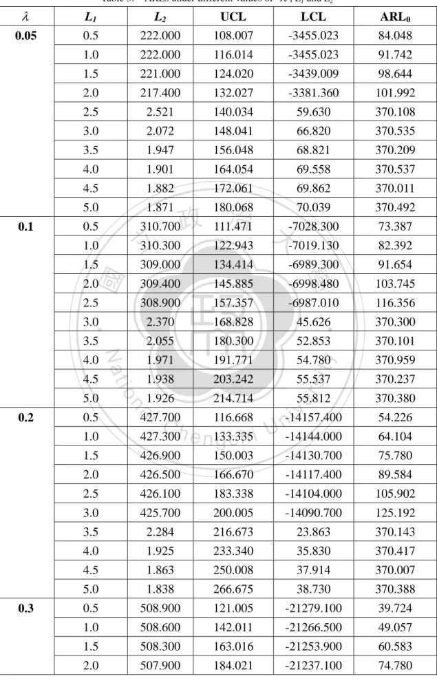
(35) where Q stands for the transition probability matrix without the (N+1)th column and row, I is the identity matrix, a 1xN matrix ‗one‘, and b is a vector with initial probability for each state, which could be obtained by satisfying the limitation of. bQ  b .. 3.4 The ARL Calculation (1). Determine ( L1 , L2 ) under Various  with ARL0 = 370 As mentioned earlier, we would like to investigate the impact of the. 政治大 is the variance of the measurement error and 立. measurement error on control charts. So we will calculate ARLs under different ratios of  2 /  2 . Note that  2.  2 is the. ‧ 國. 學. variance of the exponential random variable. First, we have to find the values of the parameters  , L1 and L2 such that ARL0 = 370. In addition, set   100 and. ‧.  2  1 . The procedure to find the values of the parameters  , L1, and L2 is：. sit. y. Nat. Step 1：Set   0.05 and L1  0.5. n. al. er. io. Step 2：By eq. (51), set ARL0  bT ( I  Q) 11  370 , since L1  0.5 then we can get L2.. Ch. engchi. i Un. v. Step 3：Let L1  L1  0.5 and L1  6 , repeat Step 2. Step 4：Let     0.1 and   0.9 repeat Step 1 - Step 3. The ARLs under different values of  , L1 and L2 are listed in Table 3.. 23.

(36) Table 3.. ARLs under different values of.  , L1 and L2. . L1. L2. UCL. LCL. ARL0. 0.05. 0.5. 222.000. 108.007. -3455.023. 84.048. 1.0. 222.000. 116.014. -3455.023. 91.742. 1.5. 221.000. 124.020. -3439.009. 98.644. 2.0. 217.400. 132.027. -3381.360. 101.992. 2.5. 2.521. 140.034. 59.630. 370.108. 3.0. 2.072. 148.041. 66.820. 370.535. 3.5. 1.947. 156.048. 68.821. 370.209. 4.0. 1.901. 164.054. 69.558. 370.537. 4.5. 1.882. 172.061. 69.862. 370.011. 70.039 治 310.700政 111.471 -7028.300 大 310.300 122.943 -7019.130 立. 5.0 0.5. 91.654. 2.0. 309.400. 145.885. -6998.480. 103.745. 2.5. 308.900. 157.357. -6987.010. 116.356. 3.0. 2.370. 168.828. 45.626. 3.5. 2.055. 180.300. ‧. 370.300. 52.853. 370.101. 1.971. 191.771. 54.780. 370.959. 1.938. 203.242. 55.537. 370.237. Nat. io. 1.926 214.714 55.812 a427.700 iv l C 116.668 -14157.400 n 427.300h e n 133.335 g c h i U -14144.000. 370.380. 1.5. 426.900. 150.003. -14130.700. 75.780. 2.0. 426.500. 166.670. -14117.400. 89.584. 2.5. 426.100. 183.338. -14104.000. 105.902. 3.0. 425.700. 200.005. -14090.700. 125.192. 3.5. 2.284. 216.673. 23.863. 370.143. 4.0. 1.925. 233.340. 35.830. 370.417. 4.5. 1.863. 250.008. 37.914. 370.007. 5.0. 1.838. 266.675. 38.730. 370.388. 0.5. 508.900. 121.005. -21279.100. 39.724. 1.0. 508.600. 142.011. -21266.500. 49.057. 1.5. 508.300. 163.016. -21253.900. 60.583. 2.0. 507.900. 184.021. -21237.100. 74.780. 0.5 1.0. n. 5.0. sit. -6989.300. ‧ 國. 134.414. 4.5. 0.3. 82.392. 309.000. 4.0. 0.2. 73.387. 學. 1.5. 370.492. y. 1.0. 180.068. er. 0.1. 1.871. 24. 54.226 64.104.

(37) 507.600. 205.026. -21224.500. 92.349. 3.0. 507.200. 226.032. -21207.700. 113.990. 3.5. 506.900. 247.037. -21195.100. 140.771. 4.0. 1.872. 268.042. 21.356. 370.217. 4.5. 1.757. 289.047. 26.209. 370.402. 5.0. 1.721. 310.053. 27.713. 370.031. 0.5. 570.000. 125.001. -28401.425. 29.028. 1.0. 569.700. 150.002. -28386.424. 37.301. 1.5. 569.400. 175.004. -28371.423. 47.931. 2.0. 569.100. 200.005. -28356.423. 61.592. 2.5. 568.800. 225.006. -28341.422. 79.145. 3.0. 568.500. 250.007. -28326.421. 101.701. 3.5. -28311.420 治 567.900政 300.010 -28296.420 大 325.011 17.381 立1.652. 130.685. 568.200. 4.0. 350.012. 19.711. 370.418. 5.5. 1.587. 375.014. 20.661. 370.760. 6.0. 1.577. 400.015. 21.146. 370.767. 6.5. 1.571. 425.016. 21.426. 0.5. 616.000. 128.869. ‧. 370.784. -35466.555. 21.132. 616.000. 157.738. -35466.555. 28.245. 616.000. 186.607. -35466.555. 37.752. io. 215.476 -35466.555 a616.000 iv l C 615.000 244.345 -35408.817 n 615.000h e n 273.214 g c h i U -35408.817. 50.458. 3.5. 615.000. 302.083. -35408.817. 120.138. 4.0. 615.000. 330.952. -35408.817. 160.575. 4.5. 1.561. 359.821. 9.871. 370.135. 5.0. 1.495. 388.690. 13.682. 370.797. 5.5. 1.474. 417.559. 14.877. 370.874. 6.0. 1.464. 446.427. 15.472. 370.365. 6.5. 1.459. 475.296. 15.789. 370.172. 0.5. 652.500. 132.734. -42618.288. 15.459. 1.0. 652.300. 165.469. -42605.194. 21.460. 1.5. 652.100. 198.203. -42592.100. 29.791. 2.0. 651.900. 230.937. -42579.007. 41.355. 2.5. 651.700. 263.672. -42565.913. 57.408. 2.5 3.0. n. 2.0. Nat. 1.5. sit. ‧ 國. 1.606. 1.0. 0.6. 370.571. 5.0. 學. 0.5. 167.930. y. 4.5. 275.009. er. 0.4. 2.5. 25. 67.249 89.884.

(38) 651.500. 296.406. -42552.819. 79.692. 3.5. 651.300. 329.140. -42539.725. 110.627. 4.0. 651.100. 361.875. -42526.632. 153.570. 4.5. 650.900. 394.609. -42513.538. 213.183. 5.0. 1.390. 427.343. 9.031. 370.110. 0.5. 678.800. 136.692. -49712.793. 11.297. 1.0. 678.700. 173.384. -49705.454. 16.314. 1.5. 678.500. 210.075. -49690.778. 23.557. 2.0. 678.400. 246.767. -49683.439. 34.020. 2.5. 678.200. 283.459. -49668.763. 49.124. 3.0. 678.100. 320.151. -49661.424. 70.944. 3.5. 677.900. 356.843. -49646.748. 102.440. 4.0. -49639.409 治 677.600政 430.226 -49624.732 大 466.918 5.453 立1.288. 147.941. 6.0. 678.800. 136.692. -49712.793. 11.297. 0.5. 696.900. 140.827. -56804.492. 8.273. 1.0. 696.800. 181.654. -56796.326. 12.449. 1.5. 696.700. 222.481. -56788.161. 18.734. 2.0. 696.600. 263.307. ‧. -56779.996. 28.191. 696.500. 304.134. -56771.830. y. 42.423. 696.400. 344.961. -56763.665. 63.838. 4.5. 4.0 4.5. 0.9. 385.788 -56755.499 a696.300 iv l C 696.200 426.615 -56747.334 n 696.100h e n 467.442 g c h i U -56739.169. n. 3.5. io. 3.0. Nat. 2.5. 學. 0.8. ‧ 國. 5.0. 393.534. sit. 677.800. er. 0.7. 3.0. 213.620 370.416. 96.065 144.560 217.537. 5.0. 1.191. 508.269. 2.775. 370.087. 6.0. 1.146. 4672.609. 6.457. 370.882. 0.5. 707.500. 145.229. -63898.983. 6.077. 1.0. 707.400. 190.458. -63889.937. 9.554. 1.5. 707.400. 235.687. -63889.937. 15.022. 2.0. 707.300. 280.916. -63880.891. 23.619. 2.5. 707.300. 326.145. -63880.891. 37.135. 3.0. 707.200. 371.374. -63871.845. 58.385. 3.5. 707.200. 416.603. -63871.845. 91.799. 4.0. 707.100. 461.832. -63862.799. 144.328. 4.5. 707.100. 507.061. -63862.799. 226.927. 5.0. 1.097. 552.290. 0.741. 370.756. 26.

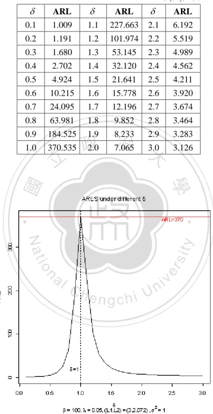
(39) 6.0. 1.079. 642.748. 2.373. 370.137. From Table 3 we could choose any combinations of  , L1, L2 to make ARL0 = 370, for example, if we set   0.05 , L1 = 3, then L2 should be 2.072 to make ARL0 = 370. Also, as the  value gets bigger, the number of the combinations of ( L1 , L2 ) to make ARL0 = 370 will be less than small  . When   0.05 , there are seven combinations of ( L1 , L2 ) that could make ARL0 = 370. But with the increase of  , say   0.9 , there are only two combinations that make ARL0 = 370.. 政治大 to check all these combinations 立 to make sure they are ―reasonable‖. The way we. Now we have the combinations of  , L1, L2 to make ARL0 = 370. Next, we have. ‧ 國. 學. check whether they are reasonable is to see if their ARL1 values are smaller than ARL0 values whenever the size of the shift  varies. Table 4 to Table 9 and Figure 4. ‧. to Figure 9 show the reasonable combinations of  , L1, L2 under ARL0 = 370 for. sit. y. Nat.   0.05 - 0.5 under   100 . To investigate the difference between small  and. n. al. er. io. large, we add one more case by setting   1000000. with   0.05 and. iv. ( L1 , L2 )  (3,2.072 ) when ARLC 0 = 370. Table 10 and Figure U n 10 show the ARLs for. hengchi. various values of  ；Table 11 lists all reasonable combinations of  , L1 and L2. Note that the ARL value under   1 is the ARL0, the rest of the ARLs are values of ARL1.. 27.

(40) Table 4. The ARL under the combination of  with   0.05 and ( L1 , L2 )  (3,2.072 ) and  2  1. . ARL. . ARL. . ARL. 0.1. 1.009. 1.1. 227.663. 2.1. 6.192. 0.2. 1.191. 1.2. 101.974. 2.2. 5.519. 0.3. 1.680. 1.3. 53.145. 2.3. 4.989. 0.4. 2.702. 1.4. 32.120. 2.4. 4.562. 0.5. 4.924. 1.5. 21.641. 2.5. 4.211. 0.6. 10.215. 1.6. 15.778. 2.6. 3.920. 0.7. 24.095. 1.7. 12.196. 2.7. 3.674. 0.8. 63.981. 1.8. 9.852. 2.8. 3.464. 0.9. 184.525. 1.9. 8.233. 2.9 治 370.535 政 2.0 7.065 3.0 大立. 1.0. 3.283 3.126. ‧. ‧ 國. 學. n. er. io. sit. y. Nat. al. Ch. engchi. i Un. v. Figure 4. The ARL under the combination of  with   0.05 , ( L1 , L2 )  (3,2.702 ) and  2  1. 28.

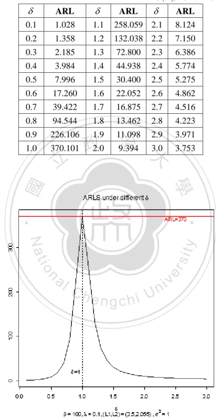
(41) Table 5. The ARL under the combination of  with   0.1 , ( L1 , L2 )  (3.5,2.055) and  2  1. . ARL. . 0.1. 1.028. 1.1. 258.059 2.1. 8.124. 0.2. 1.358. 1.2. 132.038 2.2. 7.150. 0.3. 2.185. 1.3. 72.800. 2.3. 6.386. 0.4. 3.984. 1.4. 44.938. 2.4. 5.774. 0.5. 7.996. 1.5. 30.400. 2.5. 5.275. 0.6. 17.260. 1.6. 22.052. 2.6. 4.862. 0.7. 39.422. 1.7. 16.875. 2.7. 4.516. 0.8. 94.544. 1.8. 13.462. 2.8. 4.223. 0.9. 226.106. 1.9. 11.098. 2.9 治 370.101 政 2.0 9.394 3.0 大立. 3.971. 1.0. ARL. . ARL. 3.753. ‧. ‧ 國. 學. n. er. io. sit. y. Nat. al. Ch. engchi. i Un. v. Figure 5. The ARL under the combination of  with   0.1 , ( L1 , L2 )  (3.5,2.055) and  2  1. 29.

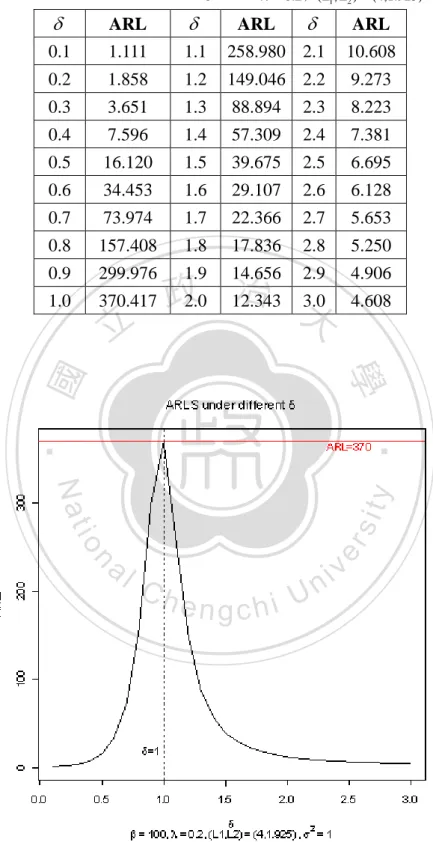
(42) Table 6. The ARL under the combination of  with   0.2 , ( L1 , L2 )  (4,1.925) and  2  1. . ARL. . 0.1. 1.111. 1.1. 258.980 2.1. 10.608. 0.2. 1.858. 1.2. 149.046 2.2. 9.273. 0.3. 3.651. 1.3. 88.894. 2.3. 8.223. 0.4. 7.596. 1.4. 57.309. 2.4. 7.381. 0.5. 16.120. 1.5. 39.675. 2.5. 6.695. 0.6. 34.453. 1.6. 29.107. 2.6. 6.128. 0.7. 73.974. 1.7. 22.366. 2.7. 5.653. 0.8. 157.408. 1.8. 17.836. 2.8. 5.250. 0.9. 299.976. 1.9. 14.656. 2.9 治 370.417 政 2.0 12.343 3.0 大立. 4.906. 1.0. ARL. . ARL. 4.608. ‧. ‧ 國. 學. n. er. io. sit. y. Nat. al. Ch. engchi. i Un. v. Figure 6. The ARL under the combination of  with   0.2 , ( L1 , L2 )  (4,1.925) and  2  1. 30.

(43) Table.7 The ARL under the combination of  with   0.3 , ( L1 , L2 )  (4.5,1.756) and  2  1. . ARL. . 0.1. 1.248. 1.1. 283.636 2.1. 13.350. 0.2. 2.501. 1.2. 178.080 2.2. 11.592. 0.3. 5.390. 1.3. 111.276. 2.3. 10.212. 0.4. 11.497. 1.4. 73.299. 2.4. 9.107. 0.5. 23.932. 1.5. 51.169. 2.5. 8.209. 0.6. 48.680. 1.6. 37.591. 2.6. 7.468. 0.7. 96.864. 1.7. 28.813. 2.7. 6.849. 0.8. 185.454. 1.8. 22.872. 2.8. 6.325. 0.9. 312.233. 1.9. 18.686. 2.9 治 370.402 政 2.0 15.637 3.0 大立. 5.879. 1.0. ARL. . ARL. 5.494. ‧. ‧ 國. 學. n. er. io. sit. y. Nat. al. Ch. engchi. i Un. v. Figure 7. The ARL under the combination of  with   0.3 , ( L1 , L2 )  (4.5,1.7565) and  2  1. 31.

(44) Table 8. The ARL under the combination of  with   0.4 , ( L1 , L2 )  (5,1.6057 ) and  2  1. . ARL. . 0.1. 1.444. 1.1. 314.295 2.1. 16.717. 0.2. 3.289. 1.2. 214.983 2.2. 14.414. 0.3. 7.348. 1.3. 140.366 2.3. 12.611. 0.4. 15.495. 1.4. 94.188. 2.4. 11.172. 0.5. 31.062. 1.5. 66.129. 2.5. 10.007. 0.6. 59.731. 1.6. 48.544. 2.6. 9.048. 0.7. 110.640. 1.7. 37.057. 2.7. 8.250. 0.8. 195.033. 1.8. 29.245. 2.8. 7.578. 0.9. 306.713. 1.9. 23.734. 2.9 治 370.418 政 2.0 19.721 3.0 大立. 7.007. 1.0. ARL. . ARL. 6.516. ‧. ‧ 國. 學. n. er. io. sit. y. Nat. al. Ch. engchi. i Un. v. Figure 8.The ARL under the combination of  with   0.4 , ( L1 , L2 )  (5,1.6057 ) and  2  1. 32.

(45) Table 9. The ARL under the combination of  with   0.5 , ( L1 , L2 )  (5.5,1.4743) and  2  1. . ARL. . 0.1. 1.719. 1.1. 344.994 2.1. 20.960. 0.2. 4.282. 1.2. 257.320 2.2. 17.946. 0.3. 9.648. 1.3. 176.364 2.3. 15.594. 0.4. 19.853. 1.4. 120.896 2.4. 13.724. 0.5. 38.153. 1.5. 85.478. 2.5. 12.214. 0.6. 69.507. 1.6. 62.736. 2.6. 10.978. 0.7. 120.966. 1.7. 47.708. 2.7. 9.952. 0.8. 199.878. 1.8. 37.435. 2.8. 9.091. 0.9. 300.394. 1.9. 30.181. 2.9 治 370.874 政 2.0 24.903 3.0 大立. 8.361. 1.0. ARL. . ARL. 7.737. ‧. ‧ 國. 學. n. er. io. sit. y. Nat. al. Ch. engchi. i Un. v. Figure 9. The ARL under the combination of  with   0.5 , ( L1 , L2 )  (5.5,1.4743) ,  2  1. 33.

(46) Table 10. The ARL under the combination of. . with   0.05 , ( L1 , L2 )  (3,2.072 ) ,  2  1.   1000000. . ARL. . ARL. . ARL. 0.1. 1.009. 1.1. 227.384. 2.1. 6.191. 0.2. 1.191. 1.2. 101.963. 2.2. 5.519. 0.3. 1.679. 1.3. 53.141. 2.3. 4.989. 0.4. 2.702. 1.4. 32.118. 2.4. 4.562. 0.5. 4.924. 1.5. 21.639. 2.5. 4.211. 0.6. 10.214. 1.6. 15.777. 2.6. 3.920. 0.7. 24.092. 1.7. 12.196. 2.7. 3.674. 0.8. 63.968. 1.8. 9.852. 2.8 治 184.429 政 1.9 8.233 2.9 大 369.922 立 2.0 7.065 3.0. 0.9 1.0. 3.464 3.283 3.126. ‧. ‧ 國. 學. n. er. io. sit. y. Nat. al. Ch. engchi. i Un. v. Figure 10. The ARL under the combination of  with   0.05 , ( L1 , L2 )  (3,2.702 ) ,  2  1 and.   1000000. 34.

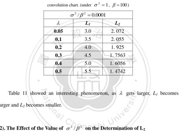
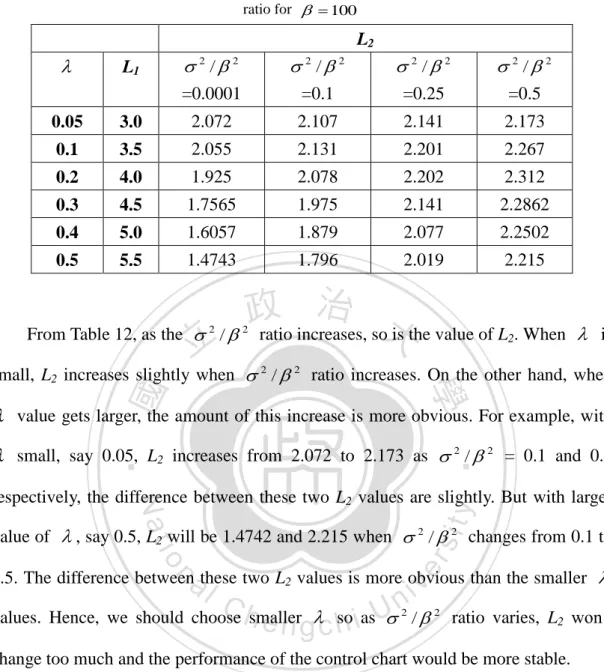
(47) From Table 4 to Table 9, the ARL1 increases as  increases to 1 from 0 but ARL1 decreases as  increases to 3 from 1; the ARL1 values are smaller than ARL0 values regardless of the size of the shift  . That is reasonable. The ARL values are very similar for small  (   100 ) and large  (   1000000 ).. Table 11. All reasonable combinations of.  , L1 and L2 for the Exponential-Normal EWMA. convolution chart. (under  2  1 ,   100 ).  2 /  2  0.0001.  0.05 0.1. L2. 治 2. 072 政 3.0 3.5 2. 大055 4.0. 1. 925. 0.3. 4.5. 1. 7563. 0.4. 5.0. 1. 6056. 0.5. 5.5. 1. 4742. 學 ‧. ‧ 國. 立 0.2. L1. sit. y. Nat. Table 11 showed an interesting phenomenon, as  gets larger, L1 becomes. n. al. er. io. larger and L2 becomes smaller.. Ch. engchi. i Un. v. (2). The Effect of the Value of  2 /  2 on the Determination of L2 According to the discussion above, we found all reasonable combinations of. ( L1 , L2 ) for l = 0.05 - 0.5 . To find out how the different ratio  2 /  2 would affect the choice of the combination of ( L1 , L2 ) , we set l = 0.05 - 0.5 、L1 = 3(0.5)5.5 with the ratio  2 /  2 = 0.0001, 0.1, 0.25, 0.5 to find L2 that makes ARL0 = 370 under   100 .. 35.

(48) Table 12.. L2 values under different combination of  and L1 with different size of the  2 /  2 ratio for   100. L2. . L1. 0.05. 3.0. 0.1. 3.5. 0.2. 4.0. 0.3. 4.5. 0.4. 5.0. 0.5. 5.5. 2 /2 =0.0001 2.072 2.055 1.925 1.7565 1.6057 1.4743. From Table 12, as the . 2. 立. 2 /2 =0.1 2.107 2.131 2.078 1.975 1.879 1.796. 2 /2 =0.25 2.141 2.201 2.202 2.141 2.077 2.019. 2 /2 =0.5 2.173 2.267 2.312 2.2862 2.2502 2.215. 政治大 /  ratio increases, so is the value of L . When 2. 2.  is. ‧ 國. 學. small, L2 increases slightly when  2 /  2 ratio increases. On the other hand, when.  value gets larger, the amount of this increase is more obvious. For example, with. ‧.  small, say 0.05, L2 increases from 2.072 to 2.173 as  2 /  2 = 0.1 and 0.5. sit. y. Nat. respectively, the difference between these two L2 values are slightly. But with larger. io. er. value of  , say 0.5, L2 will be 1.4742 and 2.215 when  2 /  2 changes from 0.1 to. al. 0.5. The difference between these two L2 values is more obvious than the smaller . n. iv n C values. Hence, we should choose hsmaller so iasU /  e n gc h 2. 2. ratio varies, L2 won‘t. change too much and the performance of the control chart would be more stable.. (3). ARL0 under Different Values of  2 /  2 and  Next, we investigate the sensitivity of the Exponential–Normal EWMA convolution chart with six different combinations of  , L1 and L2 from Table 12. Since they‘re all reasonable choices, the only thing we need to focus on is the speed they reflect to the unusual causes, which means the level of ARL1 under the same amount of shift  . Smaller ARL1 values mean that when unusual causes happened in. 36.

(49) the process, the control chart would catch it quickly, which in turn means better sensitivity. Table 13 to Table 16 list the ARLs under different size of the  in the process with different  2 /  2 ratios. Note that in the case of   1 , it indicates the ordinary convolution chart without EWMA approach. Besides, the column named ―ARL saved % ‖ is the ARL percentage saved between   0.05 and the   1 case.. ARL saved % . 立. ARL 1  ARL 0.05 ARL 0.05. 政治大. ‧. ‧ 國. 學. n. er. io. sit. y. Nat. al. Ch. engchi. 37. i Un. v.

(50) Table 13. ARLs under different combinations of  , L1 and L2 with  2 /  2  0.0001 ,   100. . 0.05. 0.1. 0.2. 0.3. 0.4. 0.5. 1. L1. 3. 3.5. 4. 4.5. 5. 5.5. 7. L2. 2. 072. 2. 055. 1. 925. 1. 7565. 1. 6057. 1.4743. 1.00374.  =0.1. 1.009. 1.028. 1.111. 1.248. 1.444. 1.719. 44.397. 97.73%. 0.2. 1.191. 1.358. 1.858. 2.501. 3.289. 4.282. 86.450. 98.62%. 0.3. 1.680. 2.185. 3.651. 5.390. 7.348. 9.648. 128.508. 98.69%. 0.4. 2.702. 3.984. 7.596. 11.497. 15.495. 19.853. 170.568. 98.42%. 0.5. 4.924. 7.996. 16.120. 23.932. 31.062. 38.153. 212.623. 97.68%. 0.6. 10.215. 17.260. 34.453. 48.680. 59.731. 69.507. 254.583. 95.99%. 0.7. 24.095. 39.422. 73.974. 96.864. 110.640 120.966 295.794. 91.85%. 0.8. 63.981. 94.544. 157.408 185.454 195.033 199.878 333.679. 80.83%. 0.9 184.525 226.106. 361.869. 49.01%. 370.396. -. 1.0 370.535 370.101. 治 299.976 政 312.233 306.713 300.394 大 370.417 370.402 370.418 370.874 立. ARL saved %. 35.24%. 1.2 101.974 132.038 149.046 178.080 214.983 257.320 308.215. 66.91%. 111.276 140.366 176.364 253.428. 44.938. 57.309. 73.299. 94.188. 120.896 200.428. 83.97%. 30.400. 39.675. 51.169. 66.129. 85.478. 156.101. 86.14%. 22.052. 29.107. 37.591. 48.544. 62.736. y. 121.692. 87.03%. 12.196. 16.875. 22.366. 28.813. 37.057. 47.708. 95.838. 87.27%. 1.8. 9.852. 13.462. er. 32.120. 1.5. 21.641. 1.6. 15.778. 1.7. 76.580. 87.14%. 1.9. 8.233. 11.098. 62.175. 86.76%. 2.0. 7.065. 9.394. 22.872 29.245 37.435 a17.836 v l C 18.686 23.734 n i30.181 14.656 i U 24.903 12.343 h e 15.637 n g c h19.721. 51.287. 86.22%. 2.1. 6.192. 8.124. 10.608. 13.350. 16.717. 20.960. 42.947. 85.58%. 2.2. 5.519. 7.150. 9.273. 11.592. 14.414. 17.946. 36.467. 84.87%. 2.3. 4.989. 6.386. 8.223. 10.212. 12.611. 15.594. 31.360. 84.09%. 2.4. 4.562. 5.774. 7.381. 9.107. 11.172. 13.724. 27.280. 83.28%. 2.5. 4.211. 5.275. 6.695. 8.209. 10.007. 12.214. 23.978. 82.44%. 2.6. 3.920. 4.862. 6.128. 7.468. 9.048. 10.978. 21.273. 81.57%. 2.7. 3.674. 4.516. 5.653. 6.849. 8.250. 9.952. 19.034. 80.70%. 2.8. 3.464. 4.223. 5.250. 6.325. 7.578. 9.091. 17.161. 79.81%. 2.9. 3.283. 3.971. 4.906. 5.879. 7.007. 8.361. 15.579. 78.93%. 3.0. 3.126. 3.753. 4.608. 5.494. 6.516. 7.737. 14.231. 78.03%. n. 38. sit. 88.894. ‧. 1.4. ‧ 國. 72.800. io. 53.145. Nat. 1.3. 學. 1.1 227.663 258.059 258.980 283.636 314.295 344.994 351.544. 79.03%.

(51) From Table 13 above, the Exponential–Normal EWMA convolution chart with.   0.05 has better performance in detecting the process mean shift on both sides compared to the ordinary convolution chart. In addition, with   1 , the ordinary convolution chart without EWMA approach is the worst one. It is particularly obvious when the process deteriorates, say   0.9 , ARL1 = 361.869, almost twice as big as the case with   0.05 . Besides, the ARL saved % by the EWMA approach is at least 35% and up to 99%. This shows the EWMA approach is extremely effective in monitoring the process.. 立. 政治大. ‧. ‧ 國. 學. n. er. io. sit. y. Nat. al. Ch. engchi. 39. i Un. v.

(52) Table 14.. ARLs under different combinations of.  , L1 and L2 with  2 /  2  0.1 , .  100. . 0.05. 0.1. 0.2. 0.3. 0.4. 0.5. 1. L1. 3. 3.5. 4. 4.5. 5. 5.5. 7. L2. 2.107. 2.131. 2.078. 1.975. 1.879. 1.796. 1.5552.  =0.1. 1.187. 1.448. 2.412. 3.951. 6.155. 9.239. 78.228. 98.48%. 0.2. 1.507. 2.056. 4.024. 7.043. 11.159. 16.624. 114.398. 98.68%. 0.3. 2.177. 3.323. 7.272. 12.849. 19.885. 28.552. 150.912. 98.56%. 0.4. 3.518. 5.918. 13.596. 23.310. 34.402. 46.885. 187.554. 98.12%. 0.5. 6.358. 11.350. 25.759. 41.688. 57.761. 74.061. 224.255. 97.16%. 0.6. 12.880. 23.008. 49.059. 73.356. 94.316. 113.169 260.926. 95.06%. 0.7. 29.089. 48.736. 93.599. 126.703 149.803 167.726 297.104. 90.21%. 0.8. 72.523. 107.259 176.359 211.529 228.798 239.419 330.987. 78.09%. 0.9 192.956. 357.977. 46.10%. 370.243. -. 1.0 370.057. 治 233.883 302.630政 318.903 320.300 318.858 大 370.516 立 370.388 370.281 370.496 370.031. ARL saved %. 32.77%. 1.2 111.095 146.206 166.584 198.525 236.219 275.461 326.041. 65.93%. 49.644. 64.435. 83.442. 107.745 137.679 224.629. 84.48%. 33.358. 44.326. 58.016. 75.684. 98.066. 177.944. 86.88%. 24.038. 32.292. 42.356. 55.343. y. 1.5. 23.342. 1.6. 16.918. 71.994. 140.061. 87.92%. 1.7. 13.006. 18.282. 24.648. 32.250. 42.011. 54.571. 110.781. 88.26%. 1.8. 10.455. 14.504. 88.591. 88.20%. 1.9. 8.699. 11.898. 71.830. 87.89%. 2.0. 7.437. 10.026. 59.095. 87.42%. 2.1. 6.496. 8.636. 11.444. 14.600. 18.516. 23.480. 49.319. 86.83%. 2.2. 5.773. 7.574. 9.963. 12.619. 15.886. 20.002. 41.721. 86.16%. 2.3. 5.205. 6.742. 8.802. 11.069. 13.835. 17.297. 35.738. 85.44%. 2.4. 4.748. 6.079. 7.875. 9.834. 12.205. 15.156. 30.966. 84.67%. 2.5. 4.374. 5.539. 7.121. 8.833. 10.889. 13.433. 27.113. 83.87%. 2.6. 4.064. 5.094. 6.499. 8.010. 9.811. 12.027. 23.965. 83.04%. 2.7. 3.803. 4.721. 5.980. 7.324. 8.916. 10.864. 21.365. 82.20%. 2.8. 3.580. 4.405. 5.541. 6.746. 8.165. 9.891. 19.196. 81.35%. 2.9. 3.388. 4.135. 5.166. 6.254. 7.527. 9.069. 17.369. 80.49%. 3.0. 3.222. 3.902. 4.843. 5.831. 6.982. 8.367. 15.817. 79.63%. sit. 34.853. er. 1.4. ‧ 國. 100.237 126.373 158.908 196.704 276.872. ‧. 57.944. io. 80.841. Nat. 1.3. 學. 1.1 242.010 276.480 278.056 301.059 327.220 350.284 359.970. n. 25.434 32.953 42.617 a19.534 l C 20.654 26.582n i v34.175 15.963 i U 28.045 13.376h e17.188 n g c h21.961. 40. 79.07%.

(53) From Table 14 above, the Exponential–Normal EWMA convolution chart with.   0.05 has better performance in detecting the process mean shift on both sides compared to the ordinary convolution chart. And, the ordinary convolution chart without EWMA approach is the worst one. Again, compare to the convolution chart without EWMA approach, ARL % saved by EWMA approach is significant, at least 32% and could go up to 99%.. 立. 政治大. ‧. ‧ 國. 學. n. er. io. sit. y. Nat. al. Ch. engchi. 41. i Un. v.