利用尺度空間二值化與累積梯度投影的方法應用於車牌字體的擷取與辨識

(1)

國立交通大學

電控工程研究所

博士論文

利用尺度空間二值化與累積梯度投影的方法

應用於車牌字體的擷取與辨識

Extraction and Recognition of License Plate

Characters Using Scale-Space Binarization and

Accumulated Gradient Projection Methods

研究生: 葉天德

指導教授: 陳永平教授

(2)

利用尺度空間二值化與累積梯度投影的方法

應用於車牌字體的擷取與辨識

Extraction and Recognition of License Plate

Characters Using Scale-Space Binarization and

Accumulated Gradient Projection Methods

研究生：葉天德

Student: Tien-Der Yeh

指導教授：陳永平

Advisor: Yon-Ping Chen

國立交通大學

電控工程研究所

博士論文

A Dissertation

Submitted to Institute of Electrical and Control Engineering National Chiao Tung University

in Partial Fulfillment of the Requirements for the Degree of

Doctor of Philosophy in

Electrical Engineering Feb. 2011

Hsinchu, Taiwan, Republic of China

(3)

利用尺度空間二值化與累積梯度投影的方法

應用於車牌字體的擷取與辨識

學生：葉天德

指導教授：陳永平

國立交通大學電控工程研究所博士班

摘要

本論文提出一個車牌字體辨識系統，此系統包含三個主要方法。第一

個方法稱為尺度空間二值化，可以用來從灰階圖像上擷取字體。此方法結

合了穩健的高斯差函數和動態二值化處理，從未知影像中直接擷取出車牌

字體。為了使擷取的處理速度加快，本論文也提出優化的方法用以縮短計

算時間。第二個方法稱為邊界投票方法，適合用來矯正字體在影像拍攝過

程中所導致的幾何型變。此方法一開始假設了許多直線，然後以投票方式

找出一條通過最多邊界點的直線當成邊界線。找到的邊界線可以幫助矯正

字體的幾何型變，因而藉此改善辨識率。第三個方法稱為累積梯度投影方

法，利用累積梯度並且轉換它們成特徵向量來識別獨立字體。這些特徵向

量稱為累積梯度投影向量，被實驗證實對雜訊及照度改變是具有穩健性的。

(4)

A License Plate Recognition System Using

Scale-Space Binarization and Accumulated

Gradient Projection Methods

Student:

Tien-Der Yeh

Advisors: Dr.

Yon-Ping Chen

Institute of Electrical and Control Engineering

National Chiao Tung University

ABSTRACT

A system consisting of three methods to deal with license plate characters recognition is

proposed in this dissertation. The first method, scale-space binarization, is suitable for

extracting characters from gray-level images. The method combines the robust

Difference-of-Gaussian function and dynamic thresholding technique to extract the license

plate characters directly. In order to speed up the extraction process, optimization methods are

also disclosed to reduce the computation time. The second method, voting boundary method,

is suitable for correcting characters from geometric deformation induced during capture

process. It assumes many straight lines candidates and detects the best one passing through

most of the edge pixels by voting. The boundary lines can be used for correcting the

deformation and improve recognition rate thereby. The third one, accumulated gradient

projection method, recognizes isolated characters by accumulating the gradient projection of

the characters and converts them into feature vector for comparison. The feature vector is

called accumulated gradient projection vector and is proven robust regardless of noise and

(5)

Acknowledgement

First of all, I am heartily thankful to my advisor, Prof. Yon-Ping Chen, whose

encouragement, guidance and support from the initial to the final stage helped me to learn

what I need from the research and made this thesis possible. And the thesis committee, Prof.

Li-Chen Fu, Prof. Kuo-Kai Shyu, Prof. Jen-Hui Chuang, Prof. Kai-Tai Song, and Prof.

Sheng-Fuu Lin, whose valuable recommendations and comments help to perfect this

dissertation.

Next, I’d like to give thank to my parents, who always give me confidence and encourage

me to persist in the thesis. Also, a deepest gratitude would be shown to my respected uncle,

Mr. Ching-Tsai Peng, who taught me always positive thinking and encouraged me all the time

especially when a bottleneck is encountered on thesis writing. Besides, I would give my best

thanks and appreciation to my best friends, Erik Lin and Patrick Lam, who supported me

during this period and gave me encouragement whenever I need help. Furthermore, this thesis

would not be accomplished without my wife’s fully support. Her understanding, trust and

assistance helped me to persist in this thesis until accomplishment.

Finally, I offer my best regards and blessings to all of those who supported and helped me

in any respect during the completion of this dissertation. Because of you, I can focus on the

(6)

誌謝

首先, 我要由衷的感謝我的指導教授陳永平老師。他多年來從頭到尾

的鼓勵、引導、及支持幫助我從研究中學得我所要的及讓這篇論文得以完

成。同時要謝謝口試委員傅立成老師、徐國鎧老師、莊仁輝老師、宋

開泰老師與林昇甫老師對此篇論文的寶貴意見與指正，使本論文更臻完

善。

其次，我要謝謝我的父母，他們總是給我信心及鼓勵，讓我可以堅持

到最後並完成這篇論文。還有，我也要向我尊敬的伯父彭清財先生表達最

深的感激，他教我要維持積極的思考，尤其是在寫作論文遇到瓶頸的時候

不斷的給我正向的鼓勵。再來我要感激我兩個最好的朋友，Erik Lin 及

Patrick Lam，他們在我寫作論文的這段期間需要幫忙的時候不斷的給予支

持及鼓勵。此外，如果沒有內人的全力支持，這篇論文也無法完成。她的

體諒、信任及協助讓我可以無後顧之憂一路堅持直到完成這篇論文。

最後，我要對所有在這篇論文寫作期間給予我支持、鼓勵及幫助的人

表達最高的敬意與祝福。因為你們的付出，讓我能夠專心於課業直到畢業

這一刻，謝謝你們。

(7)

List of Figures

Fig. 1-1 Functional block diagram of the proposed LPR system 3

Fig. 3-1 Functional block diagram of the SSB method 9

Fig. 3-2 An example of the SSB method 10

Fig. 3-3 The procedure to produce DOG Images on different observation scales 12

Fig. 3-4 An ideal unit-step edge (upper graph) and its DOG response (lower graph) 13

Fig. 3-5 Determine boundary pixels 15

Fig. 3-6 Extraction of a perfect sample character image 15

Fig. 3-7 Dynamic threshold propagation 17

Fig. 3-8 An example of dynamic threshold propagation 19

Fig. 3-9 Extraction of an imperfect sample character image 20

Fig. 3-10 Comparison to three Gaussian functions, 23

Fig. 4-1 Typical geometric transformations in LPR systems 27

Fig. 4-2 A character candidate and the bottom pixels 28

Fig. 4-3 Derivation of the voting boundary method 29

Fig. 4-4 Flow chart to vote boundary lines 30

Fig. 4-5 Compensation of geometric deformation 32

Fig. 5-1 The nature axes 37

Fig. 5-2 The nature axes and the augmented axes 38

Fig. 5-3 Gradient projection of COG point and any other pixels 39

Fig. 5-4 Accumulation of gradient projection 41

Fig. 5-5 Normalized AGPV 46

Fig. 5-6 An example comprising different blur index with Fig. 5-5 49

(10)

Fig. 6-2 Source image#2 binarization result 57

Fig. 6-3 Images used in noise analysis 58

(11)

List of Tables

TABLE I TPRE BY QUANTIZATION NOISE ANALYSIS 54

TABLE II TPREBY ILLUMINATION ANALYSIS 54

TABLE III COMPUTATION TIME COMPARISON OF THE THREE METHODS 55

TABLE IV TPRR BY QUANTIZATION NOISE ANALYSIS 59

(12)

Symbols

σ

: Gaussian function standard deviation

σ

1 : The first observation scale for Difference-of-Gaussian function

σ

2 : The second observation scale for Difference-of-Gaussian function

G(

σ

) :Gaussian function with standard deviation

σ

g1(x,y) :The Gaussian function with deviation

σ

1

g2(x,y) :The Gaussian function with deviation

σ

2 I(x,y) :Gray-level source image

I1 (x,y) :The first Gaussian blurred image for Difference-of-Gaussian function I2 (x,y) :The second Gaussian blurred image for Difference-of-Gaussian function D1(x,y) :The first Difference-of-Gaussian image

DOG(x,y) :A 2D Difference-of-Gaussian function

u(x0) :Unit step function in parallel to the y-axis with origin shifted to x= x0 Set1 :The first profile set

Set2 :The second profile set

Set3 :Non-profile set

thf :Fixed threshold for identifying profile pixels

effa(xb,yb) :Effective area of (xb,yb)

Reff :Radius of effective area of an edge

Bin1 :Total number of pixels for the first profile set

Bin2 :Total number of pixels for the second profile set

(xb,yb) :A boundary pixel

(xn,yn) :A neighboring pixel

(13)

|∇I1(x,y)| :Gradient magnitude on pixel (x,y) in the first Gaussian blurred image

(

p

)

b p b

,

y

x

:The pixel whose dynamic thresholds are assigned in the p-th iteration

Setbp :the set of boundary pixels with dynamic thresholds assigned in the p-th

iteration

Setap : the set of adjacent pixels with dynamic thresholds assigned in the p-th iteration

( ) ( )

(

xa i ,ya i

)

1

1 :the i-th pixel in Seta

1

CE :Total number of edge pixels of an isolated group

CB :Total number of non-edge(body) pixels of an isolated group

CT :Total number of pixels of an isolated group

CP :The number of edge pixels of an isolated group adjacent to profile sets

W :Width of a grouped image

H :Height of a grouped image

U :Occupancy of a grouped image

SP :Profile score of a grouped image

FIT :Set of boundary pixels falling inside a boundary line

UNDERFIT :Set of boundary pixels falling below a boundary line

OVERFIT :Set of boundary pixels falling above a boundary line

γ

(x,y) :Gray-level intensity value of sample pixel (x,y) m(x,y) :Gradient magnitude of sample pixel (x,y)

θ

(x,y) :Gradient orientation of sample pixel (x,y)

BINhis :Total number of bins of an orientation histogram

REShis :Resolution of an orientation histogram

GEhis :Total gradient energy of an orientation histogram

H(a) :The magnitude appeared on angle a of an orientation histogram

(14)

sk :The start angle of the k-th peak in an orientation histogram

ek :The end angle of the k-th peak in an orientation histogram

ath :Threshold for the maximum range of a peak in an orientation histogram

E(k) :Energy function for the k-th peak in an orientation histogram

D(k) :Outstanding energy function for the k-th peak in an orientation histogram

( )

x,y

mˆ :Projected gradient magnitude

( )

x,y

ˆl :Projected length

R(x) :The first gradient projection array T(x) :The second gradient projection array

( )

x

R~ :The first gradient projection array after smoothing

( )

x

Rˆ :The smoothed gradient projection array after binarization AGPV(i) :The i-th accumulated gradient projection vector

EC(V) :the edge count of an accumulated gradient projection vector V

C(U, V) :matching cost function of accumulated gradient projection vectors U and V

UV :Union vector of two AGPVs

IV :Intersection vector of two AGPVs

AAT(k) :The k-th axis angle of the test character

AA(i,j) :The angle of the j-th axis of the i-th standard character NN(i) :The number of nature AGPVs for i-th standard character NA(i) :The number of augmented AGPVs for i-th standard character NV(i) :The total number of AGPVs for i-th standard character

VS(i,j) :The j-th standard AGPV of the i-th character

CMC(i) :Character matching cost between test character and the i-th standard one

(15)

Chapter 1 Introduction

The license plate recognition, or LPR in short, has been a popular research topic for several decades [1]-[3],[19]. An LPR system is able to recognize vehicles automatically so that it is useful for many applications such as portal controlling, traffic monitoring, stolen car detection, and etc. Up to now, an LPR system still faces some problems concerning unknown plate size and orientation, various light condition, unexpected image deformation, and limited computation time[3].

Traditional methods for recognition of license plate characters often include several stages. Stage one is detection of possible areas where the license plate may exist. It is a big challenge to detect the plates quickly and robustly since images may contain far more information than just only expected plates. Stage two is segmentation, which divides the detected areas into several regions containing single character candidate. Stage three is normalization; some attributes of the character candidates, e.g., size or orientation, are transformed to certain values for the requirements of recognition stage. Stage four is recognition; the feature vectors extracted from the normalized character candidates can be recognized by technologies such as template matching[16], vector quantization[4], support vector machine(SVM)[15], or neural networks[5][6].

The motivation of this work originates from three limitations of traditional LPR systems. The first limitation is using simple features such as gradient energy to detect possible locations of license plates. Using these simple features may reduce the complexity of computation but may possibly lose some plate candidates because the gradient energy will be suppressed due to camera saturation or underexposure, which often takes place under extreme light conditions such as sunlight, night view, or shadow. The second limitation originates from assuming correct

(16)

orientations for both camera and license plates so that high gradient pixels in the image can be expected in the pre-defined direction. In real cases, the license plates may not always keep the same orientations in the captured images. Nevertheless, they can be rotated or slanted due to irregular roads, unfixed camera positions, or abnormal conditions of cars. The third limitation comes from blurred or corrupted characters in license plates, which may fail the LPR process in detection or segmentation stage. The characteristic is dangerous for application because one single unclear character may result in loss of whole license plate. Compare to human nature, people know the position of unclear characters because they see some characters located nearby. Human try different methods, e.g., change head position or walk closer, to read the unclear characters, or even guess it if it is still not distinguishable. This nature is not achievable in a traditional LPR system due to its coarse-to-fine architecture. To retain high detection rate of license plates under these limitations, the method in this work proposes a fine-to-coarse method which firstly finds isolated characters in the captured image. Once some characters on a license plate are found, the entire license plate can be detected around these characters. This method may consume more computation than the traditional coarse-to-fine method. However, it minimizes the probability of missing license plate candidates in the detection stage.

A challenge to do the fine-to-coarse method is recognizing isolated characters. There are few literatures discussing about isolated characters recognition due to several difficulties it has. First, it is difficult to extract orientation of an isolated character. In traditional LPR systems, the orientations of characters can be determined by the baseline [3][8] of multiple characters. However this method is not suitable for isolated characters. Second, the unfixed camera view angle often introduces geometric deformation on the character shapes or stroke directions. It makes the detection and normalization process difficult to be applied. Third, the unknown orientations and shapes exposed under unknown light condition and environment builds a bottleneck for the isolated characters to be correctly detected and recognized.

(17)

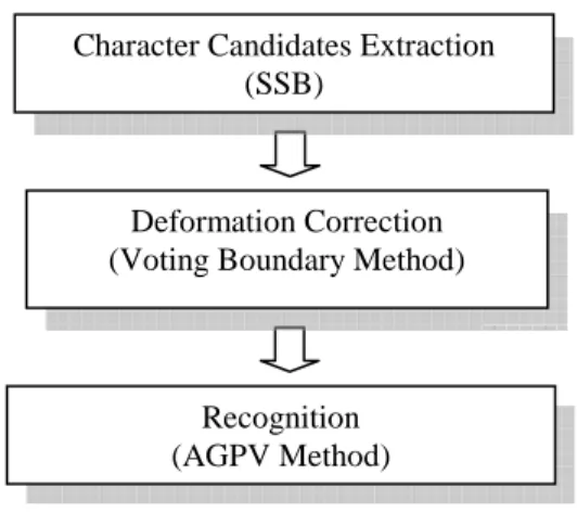
The proposed scheme to extract and recognize license plate characters has procedures as the following. First, in the extraction stage, the scale-space binarization(SSB) method which utilizes the difference-of-Gaussian (DOG) functions [9] is used to extract character candidates. The DOG function has been proven stable against noise, illumination change and 3D view point change [9]-[14]. The binarization method first localizes the character profiles on DOG image and then extracts isolated character candidates by means of dynamic threshold propagation and thresholding. Second, in the deformation correction stage, a voting boundary method is used to detect the linear boundary of character candidates, which can be used for correcting the candidates from some possible deformations. Third, in the recognition stage, the novel accumulated gradient projection vector method(AGPV method) is applied to find out the accumulated gradient projection vectors (AGPVs) of each normalized character candidate, and compare the AGPVs with those of standard letters to find the most similar one as recognition result. Fig. 1-1 shows the functional block of the proposed LPR system. The experimental results show the feasibility of the proposed method and its robustness to several image parameters such as noise, character deformation and illumination change.

Fig. 1-1 Functional block diagram of the proposed LPR system

Deformation Correction (Voting Boundary Method) Character Candidates Extraction

(SSB)

Recognition (AGPV Method)

(18)

Chapter 2 Review of Related Works

This chapter briefly describes three important techniques from which this work is motivated and constructed. First, the methods dealing with recognition of license plate characters are reviewed. Second, the useful scale-space theory and its most popular representation, difference-of-Gaussian functions, are discussed. Finally, the most popular methods doing image binarization are described and compared.

2.1. License Plate Recognition

In traditional LPR systems, there is a detection function in the first step to find possible areas that license plates may appear. The function often requires high speed feature detection and therefore is generally focused on simple features such as gradient energy or Harr-like features[51] in the image. In order to make fast detection, traditional methods often suppose a fixed camera capture angle and allow a small degree of deviation in plate size and orientation. On the detected areas, more specific rules are used to accurately localize the entire license plate and find out the histogram for binarization. Once the plate is binarized, the corresponding baseline becomes an important reference for characters segmentation and normalization. Based on the binarized plate image, the segmentation is often done by projecting the TRUE pixels onto baseline and finding the valley on the projected histogram as segmentation boundaries. For the segmented characters, the statistical features of them are extracted and fed into a statistical classifier such as template matching[16], vector quantization[4], support vector machine(SVM)[15], or neural networks(NN)[5][6], for recognition. The statistical features include some vectors such as CC(contour-crossing count)[46], PBA(peripheral ground area)[47], and CS(character shape), that are common used for recognizing license plate character.

(19)

2.2. Scale Space Theory

The concept of scale space [11] starts from the basic observation that real-world objects are composed of different structures at different scales. In other words, real-world objects may appear in different ways depending on the scale of observation. For a computer designed to detect the existence of an object in an image, it is necessary to consider all the possible scales that object may appear in the image in order to capture the interested target in the correct scale. Earlier works such as [12] and [13] have suggested that Gaussian function is the best choice for scale-space kernel. Also, in [13], the author showed that the difference-of-Gaussian(DOG) function provides a close approximation to the scale-normalized Laplacian of Gaussian,

σ

2∇2G, which was proven by detail experiment in [14] that it produces the most stable image features compared to a range of other possible image functions.

There are two additional advantages using Gaussian functions as smoothing kernel. First, its symmetric property makes it practical to decompose the two-dimensional convolution into two independent single dimensional equations. This greatly reduces the computation and shortens processing time in computing different scale images. Second, taking the Fourier transform of a Gaussian function yields another Gaussian function [17]. Consequently, it can be derived that the successive convolution with Gaussian kernel G(

σ2

) and G(

σ1

) is equivalent to convolution with G(

σ3

), where 2 2 2 1 3 σ σ σ = + ₍₁₎

Based on (1) and assumed that a Gaussian point spread function (PSF) is used to approximate the image capturing process[18], it can explain that the blur in input image can be ignored if a sufficiently large observation scale is chosen since

σ3

~

σ2

if σ2 >>

σ1

.

(20)

2.3. Image Binarization

The methods for binarization of gray-level images can be divided into two classes: global and local thresholding. Global thresholding methods generally binarize the image with a single threshold. In the contrast, local methods change the threshold dynamically over the image according to local information. The threshold for global methods is often easier to be determined than that of local methods because it focuses on the entire image. However, global methods are easily failed when the dealt image contains noise, variable illumination, or complex background. Local thresholding methods have better adaptability than global ones to deal with illumination change or complex background, however, it is difficult to decide the range of local area for threshold determination and yet still sensitive to noise.

Global thresholding methods often calculate the threshold based on histogram analysis [7], [20]-[21]. Otsu’s method [7] proposed from the viewpoint of discrimination analysis is one of the most preferred global techniques by investigators. It directly approaches the feasibility of evaluating the "goodness" of threshold and automatically selects an optimal threshold from the zeroth- and the first-order cumulative moments of the gray-level histogram. In practice, this method does not work well for the images with shadows, inhomogeneous backgrounds, and complex background patterns [22]. It is also discovered in [22] that, a single threshold or some multilevel global thresholds could not result in an accurate binary image.

Local thresholding methods generally find thresholds by statistical measurement in local areas [23]-[26] based on the principle that objects in an image provide high spatial frequency components and illumination consists mainly of lower spatial frequencies [31]. The local intensity gradient (LIG) method in [23] is one of the most popular local thresholding methods which first finds the pixels with high intensity gradient as reference of initial threshold, and then extends the threshold to whole image through region growing method [30]. It uses a

(21)

predetermined window size to calculate the regional gradient means, locates low gradient areas in the image based on the regional means, and finds edge pixels by comparing pixel’s intensity gradient with the regional means.

In general, local thresholding methods are, considered from real world situations, more accurate than global ones. However, they still suffer from two problems that usually make them unsatisfactory for investigators. First, it is difficult to give a proper size of the “local area” without prior information in the source image. Second, the methods of this class are usually more computationally expensive than the other one; it makes the local methods almost unacceptable for real-time applications.

There are still some hybrid methods to binarize the image by referring to the expected content within the region of interest (ROI). Typical applications performing hybrid binarization such as license plate recognition (LPR) or automatic document analysis, often segment the image into areas and find the areas which are most likely to be ROIs before binarization. Such systems often have faster speed and higher accuracy than general (global or loca) thresholding methods but usually require prior information within the ROI for fast detection and binarization. For example, in the LPR system [3], the author uses Haar-like features in the first step to perform fast detection and find out the ROI(license plate candidates), and then perform peak-valley analysis within the ROI for binarization of the license plates candidates. The peak-valley analysis is referring to the histogram acquired in the ROI and assumes some parameters such as number of characters, characters scale and orientation are already known. In document binarization method [28], the input image is firstly segmented into different types ROIs containing different contents such as characters or graphics or images. And specific binarization methods are applied within the ROIs based on the characteristics of the type of contents. In usual, the hybrid methods are not general enough to be applied onto different applications.

(22)

Chapter 3 The Extraction Method

The problem of character extraction is similar to that of object localization [38], where the largest bottleneck is almost all relevant factors are unknown in the source image, e.g., the scales of the objects, the condition of illumination, the complexity of the background, and the degree of blur and noise…, etc. As the scale of observation is closely related to the scale of the characters in the image, an incorrect observation scale may incorporate undesirable information and lead to undesirable extraction results [32]. In order to do extraction robustly and efficiently, we propose a scale-space binarization method, or SSB in short, to extract the characters. The extraction is started from the smallest observation scale which has best discrimination for characters sized within a certain range, for example, 16×16 to 64×64. Smaller sizes characters are discarded because they are most probably caused by noise. For larger sizes characters, a higher observation scale is preferred to minimize the probability of misinterpretation from noise. Note that the extraction on higher observation scales can be performed by utilizing the sub-sampling method to shrink the image size and enlarge the relative observation scale.

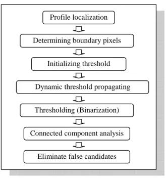
The proposed SSB method includes several functional blocks as illustrated in Fig. 3-1. First, a character profile localization block finds inner and outer profile pixels by applying a global threshold on difference-of-Gaussian(DOG) image. The DOG function used to generate the DOG image is proven to have the benefit of enhancing the edges in a digital image while minimizing the impact of noise [39]. Second, a boundary set is formed by collecting pixels neighboring to both inner and outer profile pixels. Third, the thresholds are initiated on boundary set pixels and served as the initial value for dynamic threshold propagation. Fourth, the dynamic thresholds are propagated from boundary to the remaining pixels in the image. Fifth, thresholding function compares the dynamic threshold with smoothed gray-level intensity

(23)

to binarize the image. Sixth, connected component analysis is applied to connect pixels into character candidates, and measure their preliminary features such as width, height and occupancy for the next stage. Finally, the character candidates are eliminated if their preliminary features fall beyond reasonable ranges or the profile scores are lower than general characters. An example on the simulation results of the SSB method is given in Fig. 3-2 for easy understanding. In the next sections we’ll step by step explain the behavior of each functional block in detail.

Fig. 3-1 Functional block diagram of the SSB method

3.1. Profile Localization

Profile localization, similar to edge detection, is often applied in the first stage of an image recognition process to locate pixels as the basis of segmentation or matching. Many operators can be found in literatures to detect edges or corners in an image, e.g., Sobel operator[40], Harris detector[41], or Canny detector[42]. Most of them use gradient based detection and suffer from the difficulties in noise rejection and threshold determination. The extraction method in this work utilizes the DOG functions so that it minimizes the impact of noise and

Profile localization (

Determining boundary pixels Initializing threshold Dynamic threshold propagating Thresholding (Binarization)

Eliminate false candidates Connected component analysis

(24)

makes robust extraction without prior filtering.

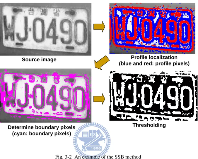
Fig. 3-2 An example of the SSB method

The profile localization consists of several steps as in the following procedures. At first, the gray-level input image, I(x,y), is respectively convolved with two Gaussian functions, g1(x,y)

with deviation

σ1

and, g2(x,y) with deviation

σ2

to get two Gaussian images, I1(x,y) and I2(x,y).

And the difference of the two Gaussian images, D1(x,y)= I1(x,y) - I2(x,y), is called the DOG

image.

The two standard deviations,

σ1

and

σ2

, of the two Gaussian functions are respectively called the first and the second observation scale. A smaller observation scale observes more details in an area but is more sensitive to noise. On the contrary, a larger observation scale is more stable against noise but may lose significant details of the interested characters or mix the interested characters with adjacent objects so that the characters become difficult to be extracted. In the

Source image Profile localization

(blue and red: profile pixels)

Determine boundary pixels (cyan: boundary pixels)

(25)

experiments we set the two scales

σ1

=1 and

σ2

= 2 for the profile extraction, which is proven by

experiments a better choice for processing 16×16 to 64×64 character sizes in general 256-step (8-bit) gray-level images.

In order to deal with larger scale characters with minimum computation time, an efficient method in Fig. 3-3 is applied by sub-sampling the second blurred image I2(x,y) by every two

pixels on each row and column to form a smaller image I2'(x,y). Then based on I2'(x,y)

calculates the Gaussian filtered image I3(x,y) and their DOG image D2(x,y), and applies the

same procedure again to localize the profile pixels. As a result, the observation scale w.r.t.

D2(x,y) is double to that w.r.t. D1(x,y).

A 2-D DOG function used to extract the characters can be expressed as,

( )

2 2 2 2 2 1 2 2 2 2 2 1 2 1 2 1 σ σ

σ

π

σ

π

y x y x e e y , x DOG − − − − − = . (2)

Consider a case that an unit step edge u(x0) exists in parallel to the y-axis(x= x0), the position of

peak response on convolving the unit step edge with a DOG function can be obtained by solving the differential equation,

( ) ( )

[

⊗ ₀

]

=0 ∂ ∂ x u y , x DOG x . (3)

Transforming into frequency domain and then taking inverse transform, the solution of (3) yields equivalent to that of the equation

(

x−x0,0

)

=0

DOG . (4)

Solving (4) to get the positions of the two peak responses at

1 2 2 1 2 2 2 2 2 1 0 2

σ

ln x x ⋅ − ± = . (5)

(26)

Fig. 3-3 The procedure to produce DOG Images on different observation scales

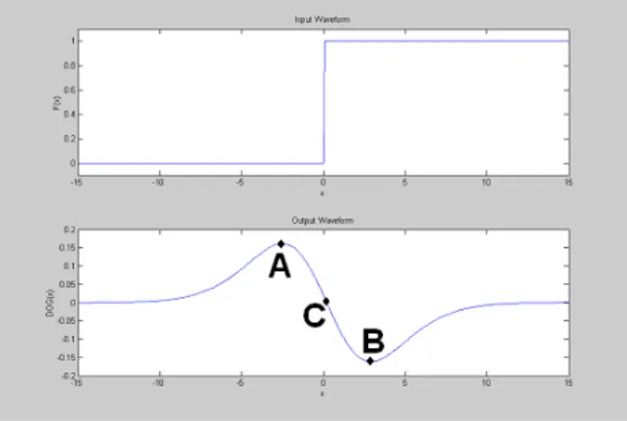
A plot by equation (5) in Fig. 3-4 on x0=0 reveals that convolution of a unit step edge with the

DOG function generates two odd-symmetrical peaks beside the unit step edge, i.e., positive peak A and negative peak B. The most valuable characteristic of the DOG function is that these peaks are quite stable even if the testing image consists of small undesirable artifacts such as noise, out-of-focus or variable illumination. Based on this result, the DOG image is divided into three sets by a fixed global threshold thf and its complementary –thf. The first set, Set1, is

composed of the pixels of D1(x,y) ≥ thf; the second set, Set2, is composed of the pixels of D1(x,y)

≤ -thf; and the third set, Set3, is the superset of the remainder containing the pixels of thf> D1(x,y)>-thf.

Set1 and Set2 are both called profile sets and have the following representation for easily D4 I1 I2 I2' I3 I4 I5 I3' I4' - - - - D1 D2 D3 source Image G(σ) G(σ) sub-sampling G(σ) G(σ) G(σ) sub-sampling sub-sampling

(27)

identification according to the way they appear. For characters having lower gray-level intensity (deeper color) than its nearby background, Set1 is also called the inner profile set because it

spreads interior characters’ boundaries. Similarly, Set2 is also called the outer profile set for the

location it appears. The two profile sets are respectively drawn in Fig. 3-5 in blue and yellow colors.

The global threshold thf is used for determining whether a change of intensity is caused by

noise or a real edge. Smaller threshold collects more pixels into Set1 and Set2, and takes more

computation time to deal with noise before extracting the characters. It is worth notify that the lowest threshold for DOG function can be set to thf=0. Although setting threshold to zero

introduces much information generated by noise, it can still retain correct extraction results because that the energy of noise in the DOG response is automatically suppressed when it appears near an edge. As a result, it is recommended to set a small threshold, e.g., thf =1, for all

the input images because it ensures reliable results can be persisted with reasonable computation time regardless of the condition of the input image. Different from some other gradient operators which would possibly lose some character candidates if a smaller threshold is given, the only drawback for giving a smaller threshold in DOG function is higher computation time consumption. From various simulation results we can tell that a wide range of threshold on DOG images can still provide reliable results on localizing the profile pixels.

(28)

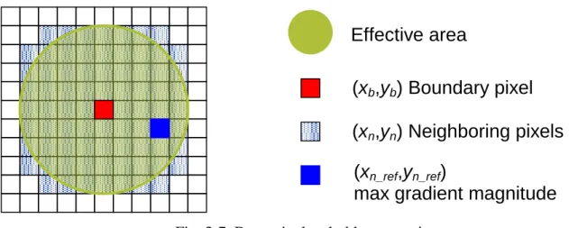
When a near-perfect input image like Fig. 3-6(a) is given for binarization, the first step is to find the corresponding two profile sets from the DOG image as in Fig. 3-6(b). It is worth to note that the pixels of the inner profile set often appear in a connected group, which is called the inner profile groups or simply profile groups. As in Fig. 3-6(c), the smallest rectangle covering the entire profile group is called the bonding rectangle of the profile group. Note that a profile group often represents the profile of an isolated character in normal case. However, it might happen that a character is broken into two or more profile groups due to special geometric distribution or noise or special lighting condition. The broken profile groups will be linked up by the connected component analysis later on to reveal the original characters.

According to (5), a constant Reff is defined to represent the radius of the effective area of an

edge (intensity change), and

        ⋅ − = 1 2 2 1 2 2 2 2 2 1 2 σ σ σ σ σ σ ln ceil R_eff , (6)

where the function ceil(x) rounds x towards positive infinity. Note that the Reff is the horizontal

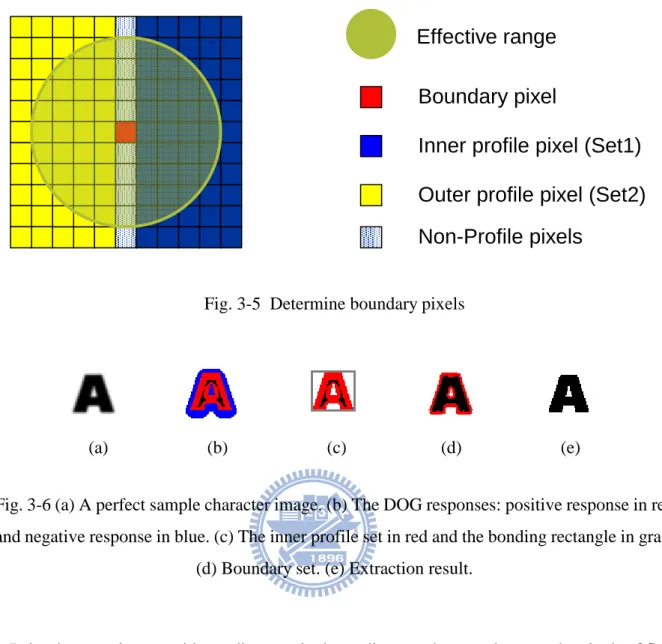
distance of AC or BC in Fig. 3-4, or equivalently the radius of the circle of effective range in Fig. 3-5. In addition to the profile sets, a boundary set SetB is formed to represent the boundary of

character candidates. A pixel pb is collected into SetB if it satisfies the following two conditions,

1. Except the zero-crossing pixels, i.e., the position C in Fig. 3-4, or the non-profile pixels in Fig. 3-5, the pixels inside the effective area of pb belong to either inner or outer profile sets.

2. The total number of pixels belongs to inner profile set and the total number of pixels belongs to outer profile set inside the effective area of pb are the same.

(29)

Fig. 3-5 Determine boundary pixels

(a) (b) (c) (d) (e)

Fig. 3-6 (a) A perfect sample character image. (b) The DOG responses: positive response in red and negative response in blue. (c) The inner profile set in red and the bonding rectangle in gray.

(d) Boundary set. (e) Extraction result.

In implementation, consider to discrete pixel coordinate and error tolerance, the pixels of Set1

and Set2 inside the effective area of pb are accumulated into Bin1 and Bin2 respectively, and pb

is collected into SetB if it satisfies the following equations:

(

)

    < − − ≥ + 2 1 2 1 2 2 1 * R Bin Bin * R round Bin Bin eff eff

π

. (7)

The pixels of SetB make up the boundaries of character candidates as in Fig. 3-6(d) and

become the base of threshold propagating in the next step. Note that the character can be extracted as in Fig. 3-6(e) after dynamic threshold propagation and binarization.

Effective range

Boundary pixel

Non-Profile pixels

Inner profile pixel (Set1)

Outer profile pixel (Set2)

(30)

3.2. Dynamic Threshold Propagation

In order to solve the global-thresholding problems such as noise, variable illumination, and complex background, and local-thresholding difficulties such as pre-determining local area size, and reducing computational complexity, a novel method using dynamic threshold propagation is proposed in this work.

Before the propagation process, each pixel in the image is assigned a dynamic threshold initialized to zero. As the process starts, the dynamic threshold on a boundary set pixel is assigned by looking for the best threshold in its neighboring area. Based on the values assigned to boundary set pixels, the dynamic thresholds are sequentially propagated to the remaining pixels through neighboring pixels. As a result, the thresholds detected around boundary pixels are able to spread out to the entire image so that the interested characters can be figured out by comparing gray-level intensity with the dynamic threshold pixel-by-pixel.

The first step of dynamic threshold propagation starts from the boundary pixels. For each boundary pixel (xb, yb), the gradient magnitude of the i-th neighboring pixel (xn(i), yn(i)) inside

the effective area, effa(xb, yb), is calculated. The pixel having maximum gradient magnitude

inside the effective area is selected as the reference pixel (xn_ref, yn_ref). In other words,

(

x

n_ref

,

y

n_ref

)

∈

effa

(

x

b

,

y

b

)

and ∇I1

(

xn_ref ,yn_ref

)

=max

(

∇I1

(

xn

( ) ( )

i ,yn i

)

, where

|∇I1(xn(i),yn (i))| is the gradient magnitude of the i-th neighboring pixel calculated by Sobel

operators as in [23]. After that, the dynamic threshold of the boundary pixel, denoted as thd(xb,

yb), is assigned by the first Gaussian gray-level of the reference pixel (xn_ref, yn_ref), i.e.,

(

b b

)

(

n_ref n_ref

)

d

x

,

y

I

x

,

y

(31)

Fig. 3-7 Dynamic threshold propagation

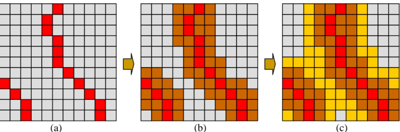
The above definition can be viewed in graphical representation as in Fig. 3-7, where the red pixel is one of boundary set pixels and the blue pixel is the one having maximum gradient magnitude inside the effective area. The reason for referring to the pixel of maximum gradient magnitude is based on the discovery that the pixels having maximum gradient magnitude often appear in the mid point of edges. It is worth to note that the calculation of gradient magnitude is referring to the first Gaussian image I1(x,y) instead of source image I(x,y) and the second

Gaussian image I2(x,y) because of the following two reasons: First, the condition of noise in the

source image I(x,y) is unknown; the gradient referring to noisy pixels is not meaningful and may

mislead the decision in finding correct threshold. Second, the second Gaussian image gives too much smoothness on boundary so that it often makes the boundary distorted after thresholding. As a result, the first Gaussian image is the best choice for gradient magnitude comparison and dynamic thresholding.

Once the dynamic thresholds of all boundary pixels have been assigned, they are iteratively propagated to the other pixels through neighboring pixels. For easily explanation, a pixel whose dynamic threshold has been assigned is called an assigned pixel.

The dynamic threshold propagation is processed by iterations. Let Setbp denote the set of

pixels

(

x_bp,y_bp

)

whose dynamic thresholds are assigned in the p-th iteration and Setap denote the

Effective area

(x

b

,y

b

) Boundary pixel

(x

n

,y

n

) Neighboring pixels

(x

n_ref

,y

n_ref

)

(32)

set of the pixels

(

x

_ap

,

y

_ap

)

adjacent to Setbp in the same iteration. Note that Setb1 stands for the

boundary set containing assigned pixels

( )

x1_b,y1_b and Setbk = Setak-1 for k>1. In the first iteration,

the dynamic thresholds on boundary pixels

(

x

1_b

,

y

_b1

)

are propagated to its adjacent pixels

(

x1_a,y1_a

)

. Let

(

xa

( ) ( )

h ,ya h

)

1 1

be the h-th pixel in Seta1 simultaneously adjacent to m boundary pixels,

denoted as

(

x

_b1

( ) ( )

i

,

y

_b1

i

)

, i=1 to m, m can be any number from 1 to 8. The dynamic threshold of

( ) ( )

(

x_a1 h ,y_a1 h

)

is assigned by averaging the dynamic thresholds of all the adjacent boundary pixels, i.e.,

( ) ( )

(

)

∑

(

( ) ( )

)

=

m i b b d a a d

th

x

i

,

y

i

m

h

y

,

h

x

th

1 1 1 1 1

1

. (9)

The first iteration ends and the next iteration starts right after all the pixels adjacent to the boundary pixels have been processed. In a general representation, the relationship for the q-th iteration is,

( ) ( )

(

)

∑

(

( ) ( )

)

= = q j m i q b q b d q j q a q a d th x i ,y i m j y , j x th 1 1 , (10) where

(

x

( ) ( )

j ,yaq j

)

q

a is the j-th pixel in Seta

q

and mjq is the total number of assigned pixels

adjacent to

(

x

( ) ( )

j ,yaq j

)

q

a . The propagation process will not finish until all the pixels become

assigned.

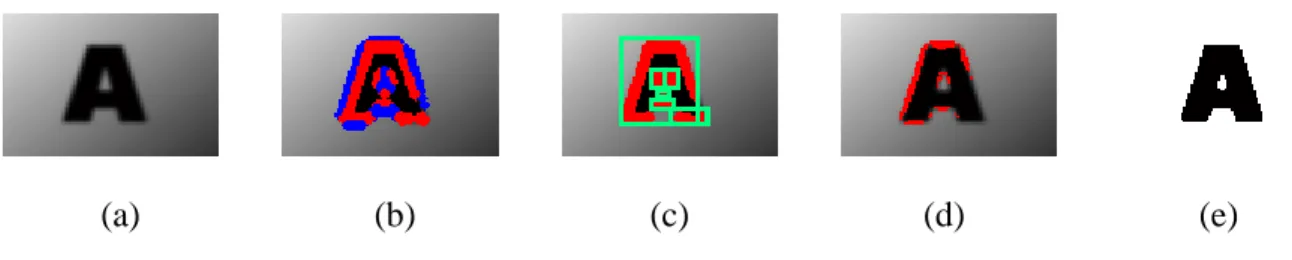
An example of the propagation can be seen in Fig. 3-8. The red pixels in Fig. 3-8(a) are the boundary pixels with the dynamic threshold initialized according to Eq. (8). The orange pixels in Fig. 3-8(b) and the yellow pixels in Fig. 3-8(c) are respectively the pixels after first and second iteration of dynamic threshold propagation.

(33)

(a) (b) (c)

Fig. 3-8 An example of dynamic threshold propagation (a) Boundary pixels (b) Assigned pixels after first iteration (c) Assigned pixels after second iteration

3.3. Thresholding and Connected Component Analysis

Based on the propagated dynamic thresholds, each pixel is converted into binary form(TRUE or FALSE) by comparing its Gaussian smoothed gray-level intensity to the own dynamic threshold. Then the connected component analysis(CCA) is applied to connect the TRUE pixels into groups named isolated groups.

During the CCA process, the TRUE pixels of each isolated group are divided into two classes and accumulated into two counters, respectively. The first class is edge pixels, which is adjacent to at least one FALSE pixel after the CCA and is accumulated into counter CE. The second class

is body pixels, which is the complementary to edge pixels, i.e., all the eight adjacent pixels are TRUE, and is accumulated into counter CB. The total number of pixels in an isolated group is

denoted CT, CT = CE + CB. For edge pixels, another counter CP is allocated to accumulate the

number of pixels adjacent to Set1 or Set2 pixels in order to give profile score to the isolated

group.

In normal cases as shown in Fig. 3-6, the profile pixels of an isolated character can be connected into an individual profile group, and the whole character should belong to an individual isolated group, too. However, it might happen that the profile group is broken into

(34)

segments due to noise or irregular light condition as the example in Fig. 3-9(a)-(d). In this case the broken profiles can still be extracted into an connected group as in Fig. 3-9(e) after thresholding and the connected component analysis.

(a) (b) (c) (d) (e)

Fig. 3-9 (a) An imperfect sample character image. (b)The DOG responses: positive response in red and negative response in blue. (c) The inner profile set in red and the bonding rectangle in

cyan. (d) Boundary set.(e) Extraction result.

3.4. Eliminate False Candidates

There are two stages elimination to filter out the false character candidates in order to minimize the computational consumption in later stages.

The first stage elimination is based on the geometric features captured by the CCA process. After the CCA, each isolated group has own preliminary features measured by its bonding rectangle, i.e., group width W, group height H, group occupancy U (pixel count w.r.t. the bonding rectangle area), U=CT/(W×H). The groups having abnormal preliminary features are

possibly caused by non-character objects such as noise or background or variable illumination and are eliminated immediately. For example, large ratio of W to H may represent a long edge or a thin line in the image; small W and H may be caused by noise or a spot; large U may stand for a solid object or shadow…, etc. General characters have a typical value for occupancy ranged in 0.3 ≤ U ≤0.8.

(35)

profiles of each isolated group, namely, the profile score SP. In ideal cases, the edge pixels found

by the CCA should be adjacent to Set1 or Set2 pixels. i.e., CP = CE . However, in real world

images, it is often not the case and most are CP < CE. Therefore, the profile score defined by SP=

CP/CE is calculated for each isolated group to evaluate how much goodness it is from the ideal

case. In our experiments, the isolated groups having SP < 0.8 is eliminated. The remaining

isolated groups form the character candidates and can be used for recognition or other purposes hereafter.

3.5. Implementation for Fast SSB

Besides a stable and accurate performance, the computational complexity of a binarization algorithm is also important in evaluating the performance. The demand for low computational complexity methods is especially strong in a real-time embedded system. In such systems they require low computational complexity methods for not only speeding up the response to external events but also reducing the power consumption. Although the computational complexity of the method presented here is higher than a global thresholding method, a good implementation can still make it computed efficiently and executed as fast as a global method. Of course, it is expected to compete with the most local thresholding methods both in accuracy and speed.

The problems to be discussed here is similar to the optimization in implementation. For the proposed method, the optimization can be considered from several aspects,

1. Simplify the convolution with Gaussian filter. 2. Use integers instead of floating points.

3. Use shifter to replace multiplier or divider.

(36)

3.5.1. Optimization in convolution

The convolution with Gaussian kernel takes much computation time because it is directly propositional to the size of the input image and the Gaussian kernel. Let W denote the width and H denote the height of the input image, and give a Gaussian kernel sized n×n. To convolve the input image with the Gaussian kernel, it needs H×W×n² multiplications and H×W×( n²-1) additions. Due to the symmetrical properties of a Gaussian function, the 2D convolution can be decomposed into horizontal and vertical direction. For each direction, n×1 dimensional Gaussian function is used so that H×W×n multiplications and H×W×(n-1) additions is required. This simplifies the complexity from O(n²) to O(n).

3.5.2. Implement by integers and shifters

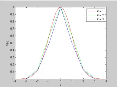
In computer systems, integer manipulation is always faster than floating points. Especially, many computer systems still have no hardware floating point processor and allow only manipulations by integers. On the other hand, multiplications or divisions often take longer computation time than simple manipulations such as addition, subtraction, or shifter; it would be preferred if they can be replaced by shifter for speeding up the computation and making the algorithm more practical on various grade computer systems. Consider to implement by integer and shifter in the program, we decide to select the Gaussian kernel as G(x)=G(y)=[1 4 8 4 1]. Fig. 3-10 gives a comparison to the three normalized Gaussian functions: selected Gaussian kernel in Gau3, ideal continuous Gaussian function(σ=1) in Gau1, and ideal discrete Gaussian function in Gau2. It shows that the selected Gaussian kernel is close to the ideal discrete Gaussian function.

(37)

Fig. 3-10 Comparison to three Gaussian functions, Gau1: ideal continuous function, Gau2: ideal discrete function, Gau3: selected kernel

The advantages of using the selected Gaussian kernel are, first, the coefficients are integers; second, all the coefficients are 2’s multiples so that the multiplications can be replaced by shifters. Based on the selected kernel, the convolution for the first Gaussian image I1(x,y) (σ1=1)

can be written as

( )

x,y

(

I

( )

x,y G

( )

x

)

G

( )

y

I1 = ⊗ ⊗ (11)

This can be achieved in program 1,

Where T [x][y] is an intermediate array, I [x][y] is the gray-level intensity on I(x,y) and I1[x][y]

is the Gaussian smoothed gray-level intensity on I1(x,y). The “<<” operator denotes the left

shifter. According to (1), the second Gaussian image I2(x,y) can be obtained by convolving I1(x,y) with the same Gaussian kernel, i.e.,

( )

x,y

(

I

( )

x,y G

( )

x

)

G

( )

y

I₂ = ₁ ⊗ ⊗ . (12)

============================================================= Program1

///////////////////////////////////////////////////////////////////////////////////////////////////////////////////////// T [x][y]=(I [x-2][y]+I [x+2][y]) + ((I [x-1][y] + I [x+1][y])<<2) + (I [x][y]<<3); I1[x][y]=( T [x][y-2]+ T [x][y+2]) + ((T [x][y-1] + T [x][y+1])<<2) + (T [x][y]<<3);

(38)

The same program1 can be used by substituting I1[x][y] with I2 [x][y] and I [x][y] with I1[x][y]. Note that the equivalent scale for I2(x,y) is σ2 = 2 based on equation (1). Finally, for

computing the DOG image, the two Gaussian images must be normalized to the same level. Therefore, the summation of the Gaussian kernel must be eliminated. The equation is written as

( )

=

( ) ( )

− ×

∑

( )

×

∑

( )

y x y G x G y , x y , x y , x I₂ I₁ D . (13) Since the

∑

( )

=

∑

( )

=18×18=324 y x y G x

G and

324 =

256 +

64 +

4 =

2

8

+

2

6

+

2

2. As a result, the

program to find the DOG image is implemented as:

It is important to check if the value in each step manipulation exceeds the full range of integers of a computer system and trim some least significant bits(LSBs) from the operands if necessary. For a 8-bit gray-level input image, the maximum value of I1(x,y) is 324×256 which

becomes 18-bit signed integers. And the maximum value of I2(x,y) is 324×324×256 which is

extended to 26-bit. For a 16-bit computer system implemented by the proposed method, the program to calculate I1(x,y) and I2(x,y) can be changed to program 3 to avoid integers overflow.

3.5.3. Use acceleration table for dynamic threshold propagation

The dynamic threshold propagation often runs over ten iterations for a typical input image

================================================================= Program3

//////////////////////////////////////////////////////////////////////////////////////////////////////////////////////////////////// T [x][y]=((I [x-2][y]+I [x+2][y]) + ((I [x-1][y] + I [x+1][y])<<2) + (I [x][y]<<3))>>2; I1[x][y]=(( T [x][y-2]+ T [x][y+2]) + ((T [x][y-1] + T [x][y+1])<<2) + (T [x][y]<<3)) >> 4;

Y [x][y]=((I1 [x-2][y]+I1 [x+2][y]) + ((I1 [x-1][y] + I1 [x+1][y])<<2) + (I1 [x][y]<<3)) >> 4;

I2[x][y]=( Y [x][y-2]+ Y [x][y+2]) + ((Y [x][y-1] + Y [x][y+1])<<2) + (Y [x][y]<<3) ;

D[x][y]= I2[x][y]- ((I1[x][y]<<4) + (I1[x][y]<<2) + (I1[x][y]>>2));

================================================================= ================================================

Program2

////////////////////////////////////////////////////////////////////////////////////////////// D[x][y]= I2[x][y]- (I1[x][y]<<8) - (I1[x][y]<<6) – (I1[x][y]<<2);

(39)

sized 640×480. It is very time-consuming if a whole-image scan is performed on each iteration. Therefore, an acceleration table is used to reduce the time required for propagation.

The acceleration table is composed of two first-in-first-out (FIFO) memories, namely FIFO A and FIFO B. When the propagation is started from boundary set pixels, the coordinates of the adjacent pixels that belong to non-boundary pixels, i.e., pixels of Seta1, are sequentially stored

into FIFO A. After a whole-image scan, all the boundary pixels are visited and the locations for the adjacent non-boundary pixels are saved. Then, in the second iteration, the propagation starts from the pixels saved in FIFOA, they become Setb2 pixels for this iteration. Again, the

coordinates of the pixels adjacent to Setb2 form Seta2 and are stored into FIFO B. The process

repeats the same flow and toggles FIFO A and FIFO B by iteration. As a result, only one full image scan is required for the first time and the computation is greatly reduced by the way.

(40)

Chapter 4 The Deformation Correction Method

In general cases, the license plate characters are often involved with certain degree of deformation when they are projected into two-dimensional images. The deformation in turns of mathematics could be composed of any transformation such as rotation, scaling, affine transform or mixed transformations…, etc. It is difficult to recognize these characters without correcting the deformation beforehand. In this chapter a novel method is discussed to correct the extracted characters in the proposed license plate recognition system.

4.1. Useful Properties for Deformation Correction

The extracted character candidates are not suitable for recognition directly because they probably undergo some geometric transformations such as rotation, affine deformations or mixed deformation…due to abnormal camera location or capture angle. The method in this section tries to eliminate the geometric transformations of character candidates and transform them into normal orientation for stable recognition. Fig. 4-1 shows some typical transformations from normal plate image in Fig. 4-1(a) such as rotation in Fig. 4-1(b), affine deformation in Fig. 4-1(c) and mixed deformation in Fig. 4-1(d). Due to the difficulties in finding invariant reference points, we utilize two useful properties for license plate characters to eliminate the undergone geometric transformations. The properties may not be sufficient to make perfect recovery from the deformation; however they can be used to detect the deformation and correct it in certain degrees to improve the successful rate in recognition.

The first property used for correcting geometric deformation of character candidates is the baseline. The baseline is an invisible line above which all the characters on a license plate are aligned. For various geometric deformations such as Fig. 4-1(b)-(d), the baseline can be used to correct a part of them, e.g., Fig. 4-1(b). However, for some other deformations, e.g., Fig.

(41)

4-1(c)-(d), it needs more information in addition to baseline to correct them for recognition. In order to correct from these complex deformations, a second property is adopted by referring to the horizontal boundary lines of each candidate. Unlike the baseline belonging to a group of character candidates, the horizontal boundary lines are the left and right boundaries belonging to a single character candidate which can be used to normalize the slant angle of each character candidate so that it can be changed to a state suitable for feature extraction and recognition.

Before locating the baseline, the character candidates are grouped by their sizes and positions. The rules of license plates [48] with an acceptable tolerance are used to check if the character candidates belong to the same license plate. The candidates obeying the rules will be grouped and considered as a single license plate. For each group of character candidates, a baseline is expected to exist below and can be found by the following methods.

Fig. 4-1 Typical geometric transformations in LPR systems

(a) Normal Plate (b) Rotational transformation

(c) Affine transformation (d) Mixed transformation

(42)

4.2. Voting Boundary Method

The voting boundary method is suitable to find boundary lines of a group of pixels in an image. It works by assuming many straight line candidates and detecting the best one passing through most of the edge pixels by voting. The method is in some respects similar to Hough transform[49] and has the same advantage with it in robust detection. However, it simplifies the computation from Hough transform by replacing the complex triangular functions with simple additions and subtractions.

Fig. 4-2 A character candidate and the bottom pixels

Before the voting boundary method, it is required to find the edge pixels in four directions, respectively top, bottom, left and right boundary pixels. The edge pixels are the most outside pixels of an image group. For example, the bottom pixels are defined as the set of pixels that first appear when searching from bottom to top on each vertical pixel line. Fig. 4-2 shows an example on how to find the bottom pixels, where the gray pixels are grouped by connected component analysis in the extraction stage and the pixels marked as ‘B’ are the bottom pixels found according to the definition above. The principle for computing the voting boundary method starts from similar triangles. Let’s see Fig. 4-3 for example, in the similar triangle pair

∆ABC and ∆ADE, it is known that a×d =

(

a+b

)

×c. Let the line

NG

be one of the bottom boundary lines of the pixel groups inside rectangle MNOP and the black circles are the

B

B B B B

B

B B

利用尺度空間二值化與累積梯度投影的方法應用於車牌字體的擷取與辨識

國立交通大學

電控工程研究所

博士論文

博士論文

博士論文

博士論文