Application of fuzzy control to a road tunnel ventilation system

(1)

~:(. • i- '

E L S E V I E R Fuzzy Sets and Systems 100 (1998) 9-28

PUZZY

sets and systems

Application of fuzzy control to a road tunnel ventilation system

P i n g - H o C h e n a, J i u n - H o n g L a i b, C h i n - T e n g L i n b'*

a Section of Control, Department o/Electronics, Chung-Shan Institute of Science and Technology, Taoyuan. Taiwan, ROC b Department ¢~f Control Engineerin 9, National Chiao-Tun.q University, Hsinchu, Taiwan, ROC

Received August 1996; revised May 1997

Abstract

This paper deals with the serious problems of ventilation system in a large road tunnel. Higher visibility and lower concentration of carbon monoxide are the key issues concerning the ventilation system. Prior to designing the fuzzy control model, a configuration layout of the ventilation system including sensing, control and traffic prediction as well is conceptually constructed. Based on the layout that offers assignments of sensors and control elements, a fuzzy logic control model is developed. Membership functions of sensor errors and control increments are physically submitted in order to set up the fuzzy logic rules. Timing and spacing filtering in terms of weighting approaches is employed in the fuzzy logic rules. A dynamic equation describing the concentration of air pollution is also given so as to cooperate with the fuzzy logic rules and to play roles in the computer simulation. The result of computer simulation involving five cases indicates that a multi-level scheme is able to solve the engineering problems. © 1998 Elsevier Science B.V. All rights reserved

Keywords: Fuzzy logic control; Tunnels; Ventilation; Simulation; Traffic prediction

I. Introduction

Moving vehicles with speed 80 km/h usually take about 10rain to pass safely along a large road tunnel with 13 km or higher in length stretched and lied on an expressway. In such a long driving duration in those large tunnels, it is necessary to provide a satisfied environment avoid o f foreseeable potential hazards. A m o n g those hazards, air pollution is greatly concerned due to its harm to vehicle drivers and pas- sengers. Research o f air pollution control in a tunnel ventilation system is thus recognized as a significant topic in case o f traffic congestion. The air in the tunnel, usually contaminated by CO, HC and dust, will reduce the visibility and more seriously cause traffic

* Corresponding author.

accidents accordingly. The objective o f air pollution control is given as follows [1]:

• To increase the visibility so that the visibility index (VI)>~40%. Actual control scheme regulates VI ~> 50% for safety reason.

• To decrease the concentration o f carbon monoxide denoted by CO so that CO < 100 ppm. Actual control scheme regulates C O < 4 0 p p m .

• To minimize electrical power consumption for cost- effective.

H o w to get started so as to meet the objectives o f pollution control problems as mentioned is a key issue o f concern. Two subsystems, Plant Monitor Control System (PMCS) and Traffic Surveillance and Control System (TSCS), are considered in the entire tunnel system [2]. If applied to the tunnel ventilation system, PMCS might deal with the operation and management 0165-0114/98/$19.00 (~) 1998 Elsevier Science B.V. All rights reserved

(2)

10 P.-H. Chen et aL/Fuzzy Sets and Systems 100 (1998) 9 ~ 8

of the tunnel installation and TSCS handles the traffic monitoring and ventilation control.

An outline of the tunnel ventilation control system using artificial intelligence [3] is referred and remod- eled in the following configuration layout for provid- ing a functional environment and thus modeling the dynamics hereafter.

Dynamic description and associated experimental curve or data are employed for computer simulation [4, 5] in which cases to be studied and simulation results to be concluded are schemed corresponding to the actual application results [6]. A thorough ventilation system including plant, dynamics, fuzzy logic control, simulation and evaluation is thus developed as follows.

IS~,o~,U us1 IS~o~21 vs2 ISecuon31 vs3

BO,~I BO/BI~ B~/BI: BO]BI~

V[ VI:~\q~ Vls~VI: VIs_VI > VI~ ._\rll~

TC TC ~FC~ TC,~TC. TG~TC~ TCtz-TQ.

WS : WS~\VS WS,~WSo WSv~\x,'~: WS~c-WSL:

CO : CO~ CO: CO, C(L

JF : JF~'~JFI, JFt ~-JF> JF:! ~JF+

DC DC~-DC~ D(L.-DC~ DC~q)C,, DC:-DC~

Entrancc ~ Fv~z) Exit

L

2. Configuration layout 12]

Fig. I. C o n f i g u r a t i o n o f facility installation.

Prior to designing the fuzzy logic controller, a configuration layout concerning the facility installation, ventilation control and pollutant dynamic should be introduced.

2.1. Configuration of facility installation

The entire tunnel in Fig. 1 is divided into four sections by three vertical shafts, VS1-VS3. Each vertical shaft is equipped with two blowers BO/BI, one of which, the BO blows off the contaminated air from the tunnel into the ambient while the other B! sucks in fresh air from ambient into the tunnel. All the sensors and control elements are installed in each section along the tunnel based on the proposed positioning assignment as follows:

Sensors

(i) Visibility index (VI): • maximum VI spot

• in front of dust collectors (DC) • in front of blowers (BL) • entrance and exit. (ii) CO counter (CO):

• in front of blowers • entrance and exit. (iii) Wind speed (WS):

• each section. (iv) Traffic counter (TC):

• 1 km aparted.

Contro[ elements

(i) Dust collector (DC): • each section. (ii) Blower (BO/BI):

• entrance and exit. (iii) Jet fan (JF):

• section #2, #3, #4.

The number of sensors for VI, TC, WS and CO are 13, 13, 12 and 4, respectively. The number of control elements for BO/BI and JF are 3 and 40, respectively. The length of each section is about 3-3.5 km. Posi- tioning of sensors and control elements will be alluded after introducing pollutant dynamic. Based on this assumed configuration of facility installation, a model of ventilation control system in detail is thus developed as below.

2.2. Configuration of ventilation control ,system

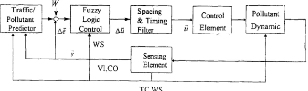
The configuration of ventilation system as shown in Fig. 2 is composed of six subsystems, i.e. sensing elements (CO counter CO; Visibility index V1;

Anemometer WS; Traffic counter TC), fuzzy logic control, spacing and timing filter, control elements (Blower BL; Dust collector DC; Jet fan JF), pollutant dynamic and traffic/pollutant predictor. Notation of Fig. 2 is defined as follows:

(3)

P.-H. Chen et al./ Fuzzy Sets and Systems 100 (1998) 928 11 Traffic/ Pollutant Predictor

l

,•

Fuzzy Logic Control WS VI,CO Spacing ~___~ff [ Control & Timing Filter Element ,[ Pollutant Dynamic Sensing I Element '

I .

TC,WS

Fig. 2. Configuration of ventilation control. W(k): Expected values of VI and CO in vector form

at each section along the tunnel:

W ( k ) = ( VII (k ) ... Vll3(k ); COl (k ) . . . C 0 4 ( k )) = (0.5,..., 0.5; 40,..., 40) (control objective) y(k): Measured data of VI and CO in vector form at each section along the tunnel:

y ( k ) = (Vll(k ) ... Vlt3(k ); C O l ( k ) , . . . ,

C04(k ))

e(k) : Control error

e(k ) = w(k ) - y ( k )

A u ( k ) : Increment of control in vector form: All(k) = (ANjF(k), A B L ( k ) , A D C ( k ) , All(k - l )) ANjv( k ) =- ( ANjv,_,o(k ), •NjF,, _20 (k),

ANjv:,_,0(k));

ZxnL(k) = (~XBL,(k), Zx~L2(k), ZxBL3(k));

A D C ( k ) = ( ADCI (k ) ... A D C 8 ( k ));

ANjF is the number vector increment of operated jet fans at each section.

A B L is the speed vector increment of blowers at each section.

u(k): Control vector (NjF, BL),NjF is the number vector of operated jet fans at each section and B L is the speed vector of the blowers in each section.

In Fig. 2, the expected values of VI and CO are to be compared with the sensing value of VI and CO and/or predicted incremental values of VI and CO. Errors of

V1 and CO are thus generated to activate the fuzzy logic control rules. Output of the fuzzy logic control

to be compensated by spacing filters and timing filters will present a more reasonable driving signal for control elements. The relationship between VI, CO and control elements is described by pollutant dynamic equation as follows.

2.3. Configuration o f pollutant distribution

Air pollution caused by moving vehicles is usually consisted of dust, smoke, carbon monoxide and hydrocarbons HC. A generalized dynamic equation for such air pollutants is given as follows [5]:

c~c C~(KSC ) c~c

~t = O---f ~x - Ur fffx + q - qs' (1) where c is the pollutant concentration, K the diffusion coefficient, (.Jr the air flow speed (or wind speed) in the tunnel, q the generation rate of pollutant concentration due to vehicle emission, and qs the removal rate of pollutant concentration due to the operation of jet fan, blower or dust collector.

The term "qs" in Eq. (1) is a significant excitation that presents the combined effect resulting from the operation of jet fan, blower and dust collector. Therefore jet fans, blowers and dust collectors are introduced as

follows.

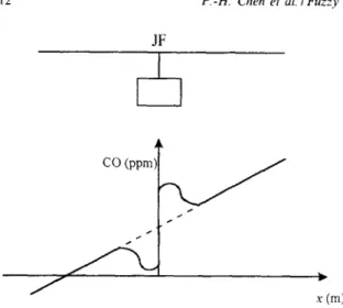
2.3.1. Jet fan

A jet fan can pump the air from its front to its back. The concentration of VI and CO is thus reduced in its front while increased in its back so as to comply with the continuity principle of mass transfer. This phenomena is illustrated by Fig. 3. The increased concentration of VI and CO in its back is further moved forward to the exit partly from piston effect of vehicle in the tunnel and partly from the tunnel wind caused

(4)

12 P.-H. Chen et al./ Fuzzy Sets and Systems 100 (1998) 9-28 JF

I

J CO (ppm] k s

z <

/ x (m)

Fig. 3. The concentration of CO in front and in back of jet fan,

by the second jet fan placed at some characteristic length behind. Therefore, the operation of jet fans has effect on the slop of longitudinal distribution curve of the concentration of VI and CO.

2.3.2. Blower

Blowers work as air exchangers to blow the polluted air out to the ambient and blow fresh air into the tunnel. The fresh air may dilute the polluted air right under the vertical shaft and thus reduces the concentration of VI and CO, especially that of CO.

Eq. (1) can be expressed by

82c 8c

k~Zx2 - Ur?~ x + q=O. (4)

Since the effect of wind speed in the second term is greater than that of diffusion in the first term, i,e.

~2C CC

ka-z2 < urn.

(5)

Therefore, Eq. (4) can be further simplified to the following linear form:

~c q or

c(x)= qx

0 x - Ur ~,. • (6) Eq. (6) shows that the concentration of pollutant is

proportional to the distance ahead and the generation rate of pollutant concentration q due to vehicle emission, but inversely proportional to the wind speed Ur. This is an approximate procedure to obtain a linear distribution curve of pollutant concentration. As to the diffusion coefficient k in Eq. (4), it may be found from the transient measurement of distribution curve of pollutant concentration.

Obviously, with known value of q/Ur [4], a linear distribution curve c ( x ) of pollutant concentration can be found and accordingly, the positioning of sensors (i.e. VI or dust collector) and control elements (i.e. blower or jet fan) can be further decided as follows.

2.3.3. Dust collector

Dust collectors can collect dust in the air and thus increase the visibility under the vertical shaft. There- fore, dust collectors have jump effect on the distribution curve of the concentration of VI rather than that of CO.

3. Positioning of sensors and control elements 13]

The positioning of sensors and control elements depends on the distribution curve of the concentration of VI and CO along the tunnel. Considering the steady state in Eq. ( 1 ),

&

- - = 0 ( 2 )

0t

if without operation of control elements,

q, =0. (3)

3.1. Positioning o f V I sensors

Obviously, the more the number of vehicles in the tunnel, the higher the pollutant concentration and the less the visibility. Therefore, a relationship between the pollutant concentration c ( x ) and the visibility index VI(x) at steady state can be approximately expressed by

V l ( x ) = VI(O) - kc(x), (7) where 171(0) is the visibility index at the entrance, and k is a coefficient.

The value of VI is expected to be higher than 50% at x = 1700 m [4]; therefore, VI(1700) = VI(O) - k q-~- x 1700=0.5, (8) Ur i.e. k q = (VI(O) - 0.5)/1700. (9) ur

(5)

P.-H. Chen et al./Fuzz}' Sets and Systems 100 (1998) 9 28

13

~

C1

f V I 1

V I 2 ~ I ~

DC2

vt(%)

50 CO (ppm)

19011 ~

i TM 1 7 0 0 m

Entrance

(m)

.,~

900m

_{.~ (m)} ~q

X

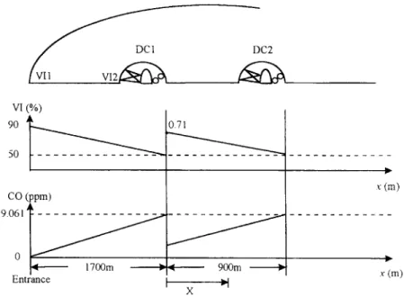
Fig. 4. Longitudinal distribution of CO and V1 pollutants at steady state.

The starting value of VI(O) can be obtained from

the VI sensor placed at the entrance. Assuming VI(O) = 0.9, then

k q =0.235 x 10-3(100%/m).

Ur

(lO)

It means every 1 m apart, the value VI of drops 0.0235%. The nominal wind speed Ur in the tunnel is about 2 m/s. The wind speed is determined by vehicle piston effect, natural wind speed and pumping effect of jet fan. As regard to the generation rate of pollutant concentration q due to vehicle emission, q can be expressed by

q = pollutant concentration per unit volume of engine emission(ppm/m 3 )

z engine emission rate (m3/s)

xvehicle occupation (%)

(11)

From the aforementioned scheme, the first VI sensor is placed at the entrance, the second one is placed 1700 m apart together with a dust collector

DCI as

shown in Fig. 4.

3.2. Positionin9 of dust collector

In order to increase the visibility of driver's vision, dust collectors are applied to absorb smoke and dust in the tunnel. Fig. 4 shows the positioning of DCI and DC2 as proposed in [3]. The efficiency of dust collector is calculated as follows:

For the location at a distance X m behind DC l,

X = x - 1700, (13)

where x isthe distance f f o m t h e entrance;then

Vl(x) = VI(X + 1700). (14)

where the emission rate is proportional to vehicle speed V by

V(m/min) = QL/O, (12)

where L is the characteristic length of the vehicle, 0 the vehicle occupation and Q the traffic flow.

From Eqs. (8) and (14),

VI(X 4- 1700)= VI(1700 +) - 0.235 x 10-3)(. (15) Let VI = 50% at X = 900 m; then

(6)

14 P.-H. Chen et al./Fuzzy Sets and Systems 100 (1998) 9 ~ 8 VSI BO1 BI1 CO (ppm) VS2 BO2 BI2 40 P P l . . . ~ ~ ~ I / Y' ' ' r , , ' , ~, [-.~ 3500m ~r~--. 2800m _...~ ,'(m) VS1 VS2 VS3 Exerance Exi|

I

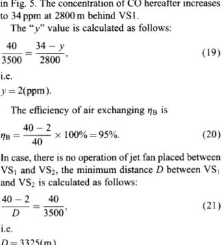
3500 m 3325 m 3325 m 2850 m

Fig. 5. The position of blowers and vertical shafts along a tunnel. i,e.

VI(1700 +) = 0.71 (right behind DCI ) (17) but right in front o f DCI, VI(1700-)= 0.5.

So the efficiency o f VI improvement t/o is 0.71 - 0.5

= 4 2 % . (18)

t/D = 0.5

Although the dust collector can improve the visibility, it cannot recover back to 90% o f VI as good as at the entrance.

3.3. Positioning of blower

Although the concentration o f CO less than 100 ppm is not harmful to vehicle drivers, the performance and control objectives o f concentration o f CO are set to be less than 50 and 40 ppm, respectively. According to what proposed in Ref. [4], a distribution curve o f concentration o f CO along a 6300 m (i.e. 3 5 0 0 + 2 8 0 0 ) tunnel is given as follows:

At the location 3 5 0 0 m away from the entrance, BOI/BII in vertical shaft VSI reduce the concentration o f CO from 40 ppm to some extent say " y " ppm as

in Fig. 5. The concentration o f CO hereafter increases to 34 ppm at 2800 m behind VS 1.

The " y " value is calculated as follows:

40 _ 3 4 - y (19)

3500 2800 ' i.e.

y = 2(ppm).

The efficiency o f air exchanging t/B is 40 -- 2

r i b - - - × 1 0 0 % = 9 5 % . (20) 40

In case, there is no operation o f jet fan placed between VS1 and VS2, the minimum distance D between VS1 and VS2 is calculated as follows:

40 - 2 40

D -- 3500' (21)

i.e.

D = 3325(m).

Fig. 5 shows the positioning o f blowers or vertical shafts along a tunnel with 13 km in length.

(7)

P.-H. Chen et al./Fuzzy Sets and Systems 100 (1998) 9 28 15 Entrance

A

/ / i A --ID,- B _ J / ' \ C ~ / - E l / J J v x (m) Fig. 6. The pollutant concentration for a single vehicle passing through the tunnel.

level change over a period of time. This is the reason why the fuzzy logic control (FLC) approach is employed in the controller of this ventilation system. There are three inputs for the FLC, i.e. nominal input, predicted input and sensor feedback input. The nominal input of FLC is the expected values of VI and CO. The predicted input, from the traffic predictor, is the predicted increment of V1 and CO. The sensor- feedback input, from the sensors, is measured values of VI and CO. The output of FLC are ANjv, the num- ber vector increment of jet fans and ABL, the speed vector increment of blowers. The difference of VI (or CO) as denoted by AVI (or ACO) is obtained by AVI : measured V I - (expected VI + predicted

incremental V1). (22)

A VI, ACO accompanied with A WS will determine ANjF, the number vector increment of jet fans and ABL, the speed vector increment of blowers by means of inference of FLC algorithm. The objective of FLC is to keep the level of VI and CO as required in Fig. 7.

3.4. Positionin.q of jet fan 4.1. Membership functions of sensors A VI, ACO

and A WS A single vehicle passing the spot "A" in the tun-

nel will generate a distribution curve of pollutant concentration just like an impulse response as shown in Fig. 6. As the time elapses, the curve will propagate forward as shown by the dotted lines in Fig. 6. There- fore, for a single vehicle passing through the tunnel, its resulting distribution curve is a combination of each distribution curve, say "A", "B", "C" and so on. Furthermore, for a series of vehicles passing through the tunnel, its overall resulting distribution curve of pollutant concentration is a combination of that of each vehicle. The overall resulting curve of pollutant concentration is approximately a linear curve starting from the entrance. This is the reason why jet fans are uniformly distributed along sections #2, #3, #4 rather than section #1.

4.1.1. Membership fimction of A V1

The nominal value of VI is set at 50%, the partition boundary is set at 4-20% with respect to the nominal value 50%. Therefore, the partition upper bound is 70% and lower bound is 30%. The notation of fuzzy term sets is defined as follows:

PB = Positive Big ( ~> 60%) PM = Positive Medium (50-70%) Z = Zero ( 4 0 - 6 0 % )

NM = Negative Medium (30-50%) NB = Negative Big (~<40%)

The membership function of sensors A VI is defined in Fig. 8.

4. Fuzzy logic control (FLC)

In order to save power consumption, the control of jet fans and blowers is not continuous but subject to

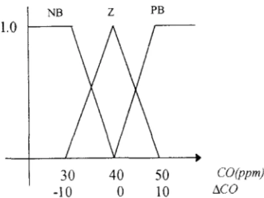
4.1.2. Membership functions of A CO

The partition boundary of CO is set at + 10 ppm with respect to the nominal value 40 ppm, i.e. the control objective. The upper bound 50 ppm is a satisfying

(8)

16 P.-H. Chen et al./Fuzzy Sets and Systems 100 (1998) 9 28 1.0 Entrance co VS 1 VS2 VS3 Exit , DC~ DC3 DC4 DC~ DC~ DC, DC~ 40PPM VI 5O% Sect.1 i i

I i Sect.2 Sect.3 Sect 4

, }

Fig. 7. The objective of FLC of CO and VI at steady state.

_ NB NM Z PM PB

30% 40% 50% 60% 70% lq(%)

-20% - 10% 0 10% 20% ,~ l/'~% )

Fig. 8. Membership function of A VI.

1.0 NB NM Z PM P B

1 pB(fws)

o5

,5

2.5 3,5 45

ws

-2 -1 0 1 2 AWS

Fig. 10. Membership function of AWS.

1.0 NB Z PB 3O 40 50 -10 0 10 CO(ppm) ACO

Fig. 9. Membership function of ACO.

level of CO concentration. Higher than 50 ppm is re- garded as a serious level of CO concentration. Fig. 9 shows the membership function of ACO.

4.1.3. Membership functions of A WS

The wind speed in the tunnel is usually 2 - 3 m/s. The nominal value of WS is set at 2.5 m/s with 4-2 m/s for upper bound and lower bound. The wind direc- tion is reversed if A WS < - 2 . 5 m/s. Fig. 10 shows the membership function of A WS.

4.1.4. Membership functions of A BO

The air flow rate in the tunnel just in front of vertical shaft VSI is assumed 95.8 m3/s. The air flow rate blew out by BOl is assumed 92 m3/s [4]. Therefore, the air exchanging ratio ~/B is

92

qB -- - - -- 96%. (23)

95.8

In other words, there is still 4% residual air remaining in the tunnel. Assuming the characteristic radius Rc of

(9)

P.-H. Chen et al./Fuzzy Sets and Systems 100 (1998) 9-28 17 1.0 _ ~ NM Z PM PB

/

V

\/

\

.

31 92 153 214 275 Qo(m3/s) -122 -61 0 61 122 6(_)0 1.0 NB NM 28 83 -110 -55 Z PM PB 138 193 248 0 55 110 Q, (m3/s) AQ, Fig. I 1. Membership function of AQo.

the tunnel is 4.5 m, then its cross section Av is

Av = ~R~ = 63.6 m 2. (24)

For the nominal wind speed V to be 2.5 m/s, the tunnel air flow rate QT is

QT =ATV = 159m3/s. (25)

Assuming a vertical shaft with radius r of 3 m, its cross section Avs is

Avs = rtr 2 = 28.3 m 2. (26)

The air flow rate Qvs in the vertical shaft is

Qvs = QTt/B = 153 m3/s. (27)

The air flow speed in the vertical shaft is

Vvs = Qvs/Avs = 153/28.3 = 5.5 m/s. (28) The wind speed is 2.5 m/s normally with upper bound 4.5 m/s. The percentage of wind speed change qw is

4.5 - 2.5

r / w - - - × 1 0 0 % = 80%. (29)

2.5

Therefore, the upper bound of flow rate in the tunnel Qu is

Qu = Qv x 1.8 = 275(m3/s). (30)

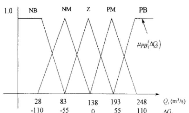
The membership function of ABO is thus given in Fig. 11. Since the air pressure in the tunnel is higher than that of the ambient air, flow rate is Qi of the blower BI is less than that of BO by almost 10%. The membership of AQi is thus given in Fig. 12.

Fig. 12. Membership function of AQi.

4.1.5. Membership functions of ANjv

There are totally 40 jet fans positioned along the tunnel with 10's for section #2, 10's for section #3, and 20's for section #4. The nominal number of operated jet fans is 4's for section #2, 4's for section #3, and 8's for section #4. The membership function of ANjF is thus given in Fig. 13.

4.2. Inference of FLC controller

Basically, the control model of a tunnel ventilation system is a MIMO system since the operation of jet fans has effect on the blower control. In the following simulation, a sequence of steps in each sampled time interval is recommended as below:

• To select ANjF by inference of FLC. • To calculate the air flow (or wind) speed.

• To update the coefficient of pollutant dynamic equation.

• To calculate the longitudinal distribution of pollutant concentration.

• To select ABO/BI.

In this way, the sophisticated MIMO system may be reduced to a two-MISO system that has same inputs

A VI, ACO and A WS but different outputs ABO/BI

and ANjF, respectively, as shown in Table I. Table 1 shows the inference of FLC controller for both blower speed control ABO/BI (i.e. air flow speed) and number control ofjex fans ANjF. Table 1 shows 37 rules rather than 75 rules since in some cases the level of CO is not taken care. Two rules R1 and Re are selected from Table 1 to show the inference procedure of FLC as follows:

Rl: IF AV1 is NB and AWS is NB and ACO is PB

(10)

18

1.0

P.-H. Chen et a l . / F u z z y Sets and Systems 100 (1998) 9-28

NB NM Z PM PB 7 Section II,III l 2 3 4 5 6 7 ?~r -3 -2 - 1 0 1 2 3 , ~ r 1.0 NB NM Z PM PB Section IV 2 4 6 8 10 12 14 tVJF -6 -4 -2 0 2 4 6 ~L¥JF

Fig. 13. Membership function of ANJF.

Table I Inference of FLC controller A WS A VI NB NM Z PM PB NB PB, PM, PM PM NM PM PM Z Z Z PM PB, PM, PM Z,Z, NM PB Z, NM, NM NM PM PM PM, PM, Z PM P M , Z , Z Z Z Z Z NM NM NM NM NM NM, NM, NB Note: A C O is PB, A C O is Z,/',CO is NB. R2: IF A V I is NB and A W S is NB and A C O is Z THEN ANjF is P M .

Based on the following definition: Input errors ei (i = 1,2,3):

el = A V I = VI - V/tel, V/ref = 5 0 % , (31) e2 = A WS = WS - mgref, WSref = 2.5 m/s, (32)

e3 = A C O = CO - COrer, COrer = 40 ppm, (33)

ei are error o f sensing values. Linguistic term set o f each error: Tel = {x, Ix1 E {NB, NM, Z, PM, PB} } Te2 = {x2 Ix2 E {NB, NM, Z, PM, PB} } Te3 = {x 3 [x 3 E {NB, Z, P M } }

are linguistic term set o f each error. Membership o f each error:

/-2X, (ei)[i-1,2,3,

I~r,.,(ei) = V IXx, (ei).

x,

Fuzzy singletons:

1, e i = c O ( i = 1,2,3), A ( e i ) = O, ei7 keO

where e0 is the measured crispy value.

(34)

(35)

(36)

(37)

(38)

(39)

(11)

P.-H. Chen et aL /Fuzzy Sets and Systems 100 (1998) 9-28 "~9 R1 el e2 e3 r I = ( u p B ( e l ) A A ( e l ) ) A . . . (/-tpB ( e 3 ) A A (e3)) rlAI~NM (Y) y = A B O / B I ( o r A N j F ) ... F1 ]

"

t

I A u

Fig. 14. Defuzzification scheme.

An intersection M(ei) of the singleton and membership functions is found by

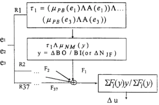
mTei(ei) & I~T~(ei) AA(ei)li=l,2,3. (40) For rule RI as shown in Fig. 14, by using max-min algorithm, the degree of fire (DOF) ~1 is obtained by

3

~1 : A MT~'i(ei) (41)

i

4.3. Defuzzification

Using the DOF z" 1 to intersect the membership function of control element #r,(Y), a profile of control function F1 (y) is obtained by

F1 (y) = Z'I /~ #T,(Y). (42)

Combining rules R1 and R2, a resultant function of control F l ( y ) can be found by

2 2

F ( y ) = V Fj(y) = V [ z j A//T,(y)]. (43)

j = l j = l

The above inference is defined in terms of Mamdani's minimum operation rule. Extending to 37 rules of FLC, the resultant function of control is obtained sim- ilarly as

37

F ( y ) = V [ z j A flT,(Y)]. (44)

j=]

Eq. (44) shows a resultant profile of control function

F ( y ) after finishing the inference of FLC.

The control increment Au is then acquired in terms of COA (center of area) approach as follows:

Au -- ~ F ( y ) y (45)

~ F ( y )

5. Spacing and timing filter for number control of working jet fans (or air-flow control of blowers)

Any one of the measures of A VI, A WS, ACO

varies with the location along the tunnel and the time. It is appropriate to express them by AVl(x,t), AWS(x,t), ACO(x,t), respectively. In wide sense, each control element ANjF or ABO/B1 is not determined exclusively by its local corresponding sensing A VI, A WS, A C O but also counted on the ones in front and the time elapsed as well. Therefore, a spacing/timing filter is thus added on to improved its performance.

5.1. Spacing filter

5.1.1. Sectional average o f AVI (or AWS, A C O vice versa)

The sectional average of A VI is given as follows:

AVIAv, i __ )-£~=1

A V/,.,j

k (46)

where AVInv, i is the averaged VI value of section

# i, AVIij the value o f j t h VI in section # i and k the number of VI sensors in section # i.

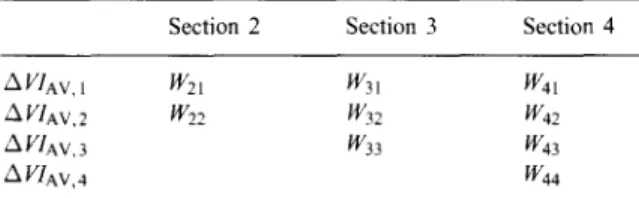
5.1.2. Weighting assignment

After assigning the weighting factors as in Table 2, a spacing filter is constructed as given by

i

AVIs'i = Z Wi'jAVIAv'j

(47)

j-1

where A VIs, i is A VI of section # i after the treatment of space weighting.

5.2. Timing filter

Combining A VI(x, k) and A VI(x, k - 1 ) with time weighting, a timing filter is developed as follows:

A VIt(x,k ) = W_l A VI(x,k - 1 ) + WoA VI(x,k ).

(48)

(12)

20 P.-H. Chen et a l . / F u z z y Sets and Systems 100 (19983 9-28

Table 2 Weighting table

Section 2 Section 3 Section 4

A V1AV, 1 W21 W31 W41

/k VIA v, 2 W22 W32 W42

A VIAv, 3 W33 W43

A V1AV ' 4 W44

7. Computer simulation of FLC ventilation system

7.1. Simpl!fied assumption

5.3. Resultant filter

The resultant filter is composed of spacing and timing filter as follows:

A U ] R , i = WssAVIs, i 4- W t A V ] t , i , (49) where /XVIR, i is the resultant VI of section # i after spacing and timing filter, Ws the weighting factor for sectional spacing filter, Wt the weighting factor for sectional timing filter, AVIs, i : A VI of section # i after space filtering and AVIt, i : A V I of section # i after time filtering.

6. Traffic/pollutant predictor

The traffic in the tunnel is usually monitored by vehicle occupation 0, traffic flow Q and associated change rate A0 and AQ in each measured interval. Therefore, a traffic monitoring vector M is introduced by defining

M = (0, A0, Q, AQ>, (503

where 0 is the vehicle occupation (%) and Q the traffic flow (number of vehicle/min).

Neglecting the diffusion term and time derivative term in Eq. (1) at steady state, Eq. (1) is simplified and expressed as follows:

c~c _ q - qs (51)

~x ur

It is obvious from Eqs. (6) and (51) that the higher traffic flow Q, the more the pollutant generation rate q and the higher the value of ~c/Ox, spacing rate of pollutant concentration. Jet fans and blowers are thus applied here to remove the pollutant towards the exit. This is an approach to show how the traffic/pollutant predictor works to predict the pollutant concentration in advance based on traffic measures.

As introduced in Section 2.1, there are four sensing elements, i.e. VI (visibility index), CO (CO counter). W S (wind speed), TC (traffic counter) and three con- trol elements, i.e. DC (dust collector), BO/BI (blower) and JF (jet fan). Indeed, the computer simulation will be too huge to be simulated if sensing elements and control elements are all included to cover the longitudinal space of the tunnel and time duration of our concern. Therfore, it is necessary to simplify the approaches of control based on actual physical meaning as follows:

• Operate three blowers (BO/BI) at nominal speed simultaneously if the number control of working jet fans can manage the pollution problems. Otherwise, increase BO/BI to higher speeds, say PM or PB. • Control the number of working duct collectors

(DC) to be synchronized with that of working jet fans due to the linear relationship between VI

(effected by DC) and CO (effected by JF). • Focus on the number control of working jet fans.

Define the multi-level control by changing membership function partition, FLC rules or speed of BO/BI to go with working jet fans in terms of the survey of simulation cases.

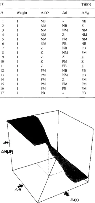
A simulation scheme is thus simplified by assigning 17 rules for FLC in Table 3 with A0 (traffic occupation) and ACO as input and ANjv as output. The following simulation is composed of 10 steps as follows:

Step 1 : Generate the traffic flow pattern (associated with TC) by random signal generator at rush hour, say AM 6:00-8:00 and PM 16:00-

19:00 as shown in Figs. 16(a) and 17(a), Step 2: Set initial number Njv of working jet fans. Step 3: Find wind speed by Njv (piston effect is

neglected).

Step 4: Find occupation 0 in terms of traffic counter TC.

Step 5: Find the generation rate of pollutant concen- tration q based on Eq. (10).

Step 6: Find CO by Eq. (6) and A C O as well. Step 7: Find VI by Eq. (13) and A V I as well. Step 8: Estimate occupation 0 by Eq. (12) and A0

(13)

P.-H. Chen et al./Fuzz), Sets and Systems 100 (1998) 9 ~ 8 21 Table 3

General-task FLC rules

IF THEN

H Weight ACO AO ANjF

1 2 3 4 5 6 7 8 9 10 l l 12 13 14 15 16 17 NB * NB NM NB Z NM NM NM NM Z NM NM PM NM NM PB NB Z NB PB Z NM PM Z Z Z Z PM Z Z PB Z PM NB PB PM NM PB PM Z PM PM PM PM PM PB PM PB * PB 7.2. Cases to be studied

There are five cases to be concerned in the computer simulation:

Case 1: Select hours of traffic jam at AM 6:00 & PM 18:00 and apply the FLC rules table in Table 3, then see if the objective of CO <<. 50 ppm and VI >~ 40% reaches or not.

Case 2: Change partitions of membership functions for both A C O and A VI (gain control in other words) and see if the result improves or not.

Case 3: Select one of the most serious problem with higher reverse wind speed at rush hour AM 6:00 and PM 18:00, then check the FLC rules in Table 3 works out or not.

Case 4: Select another serious problem with higher occupation and lower traffic speed (i.e. traffic congestion), then check the FLC rules in Table 3 works out or not.

Case 5: If both Cases 3 and 4 are unable to meet the control objectives for VI and CO, then modify the FLC rules in Table 3.

AN[JFI

Fig. 15. 3D surface of FLC.

/kCO

Step 9: Find ANjF by A C O (from step 6) and A0 (from step 8).

Step 10: Return to step 3.

The above general-task FLC rules in Table 3 gen- erates a 3D hyperplane surface of FLC as in Fig. 15.

7.3. Simulation results

Fig. 16 shows a paradigm of generalized simulation results with traffic occupation pattern 0 assigned in Fig. 16(a), total number of working jet fans NjF in Fig. 16(b), CO(ppm) concentration in Fig. 16(c) and VI(%) visibility in Fig. 16(d). All the figures are plotted with respect to 24 h time frame.

In order to show the distribution of CO concentration in each section along the tunnel at various time, a 3-D plot of CO vs. time and tunnel sections is given in Fig. 17. Fig. 17 points out that CO concentration sticks up from the allowable objective level of CO concentration at section 1, PM 18:00. This is a generalized case study, called case 1. Obviously, the case 1 result is not so satisfied as expected.

Changing the membership function of A CO and A0 from 500 partitions to 400 partitions, an improvement over case 1 is obtained as shown in Figs. 18 and 19. This is the case 2. CO concentration is satisfied along the tunnel at any time.

In case of serious reverse wind speed, approaches of case 2 no more works out. Figs. 20 and 21 show serious CO pollution. This is the so-called case 3.

(14)

22 P.-H. Chen et al./Fuzzy Sets and Systems 100 (1998) 9-28

(a) sita (occupation)

o~t ' - ' ' ' -q

0 5 10 15 20 24

(b) N (Jet fan number)

401-20I , ~ r r o [ - } ~ n ~ m l ~ l q m n n l - l q m ~ l - l l q [ q f f l ~ n ~ .~ 0 5 10 15 20 24 (c) CO (ppm) i I ~ 7 - O E , ~ I I _ I 1 . _ - - 0 5 10 15 20 24 (d) Vl (%) 0.5 0 ~ 0 5 10 15 20 24

- : Average value of section#I, -- : Average value of section#2

Time(hr) : : Average value of section#3, -. : Average value of section#4

Fig. 16. Simulation results (Case I),

60, 40, E v 0 o 20, 0 , 1 ~ - n ~ ' ~ I " Section 24 4 0 5 Time(hr) Fig. 17. CO vs. time and tunnel sections (Case 1).

(15)

P.-H. Chen et aL /Fuzzy Sets and Systems 100 (1998) 9 ~ 8 23 (a) sita (occupation)

. . . . t

0 5 10 15 20 24

4°t

.

i

200[ 71nnn~r~II~]VIfIn57-nfflNnrIrlf]FIr~

0 5 10 15 20 24 (c) CO (ppm) I E i i ]

5ol

0 0 5 10 15 20 24 (d) Vl (%) I ] ] T i o.5 ~ ~ ~ ~ . . . I I I I I . O0 5 10 15 20 24

Time(hr) : : Average value of section#3, -. : Average value of section#4

Fig. 18. Simulation results (Case 2).

Section 0 Time(hr)

Fig. 19. CO vs. time and tunnel sections (Case 2).

(16)

24 P.-H. Chen et al./Fuzz)' Sets and Systems 100 (1998) 9-28

0 5 F ' ' ' - - ' " 4

0 5 10 15 20 24

401 , -- , T , 20 t 0 5 10 15 20 24 (c) CO (ppm) 0 5 10 15 20 24

°:t

₀ (d) VI (%) F b i 5 10 15 20 24

Time(hr) : Average value of section#& -. : Average value of section#4

80- 60. &40.. d o 20, 0 ~ 1 2 _~ " -~~15 "" ,i 24 Section 4 0 Time(hr)

(17)

P.-H. Chen et al./Fuzzy Sets and Systems 100 (1998) 9-28 25

( a ) sita ( o c c u p a t i o n )

0 L I l ~ ' ~ ' i I k " i l ~ ~ /

0 5 1 0 15 20 24

20401 ~ ] ~ ] ~ r-~ m F--'~ ~ [ ~ [ ~ r - m ' ' ' ~ - - ] o . . . . - - ~ , ~ F ] ~ r ~ r ~ I ~ 0 5 10 15 20 24 (c) CO (ppm) 50 < ' - --~- , 0 0 5 10 15 20 24 (d) Vl (%) t __ i i -- [ 0.5 .:. _ _ . _ 7 . - . - . . / / ~ 0 i _ _ i _ i _ __ _ . 0 5 10 15 20 24

- : Average value of section#I, -- • Average value of section#2

" : Average value of section#3, -. • Average value of section#4

Time(hr)

1oo.. ... ~

! ... ! "

i .... -:27"- ""-i. "':'-.

~.

-'~ ~

"

"'~. "i".. :

. . . : . - "" 20

S e c t i o n 4 0 Time(hr)

(18)

26 P.-H. Chen et al./Fuzzy Sets and Systems 100 (1998) 9 28

.

0 5 10 15 20 24

2o -

o

I[ nmnF-i Fimr] n

0 5 10 15 20 24 (c) CO (ppm) i 0 5 10 15 20 24 (d) Vl (%) 0.5[- 0 J i B __ i _ i 0 5 10 15 20 24

- A v e r a g e value of section#I, -- : Average value of section#2 Time(hr)

• • Average value of section#& -. : Average value of section#4

Table 4

Heavy-task FLC rules

IF THEN

H Weight ACO AO ANjF

1 2 3 4 5 6 7 8 9 10 11 12 13 14 15 16 17 NB , NB NM NB Z NM NM Z • NM Z NM NM PM NM NM PB NB Z NB PB Z NM PM Z Z PM • Z PM Z Z PB Z PM NB PB PM NM PB PM Z PB • PM PM PM PM PB PM PB * PB

Furthermore, traffic congestion with higher occupation and lower traffic speed is considered to be case 4. Figs. 22 and 23 show tremendous contamination from CO concentration.

The case combining cases 3 and 4 presents the most serious situation for ventilation control. It is necessary to modify the FLC rules in Table 3 accompanied with changing membership function partition as case 2. The new FLC rules is given in Table 4 for this kind o f heavy task.

Observing the difference between Tables 3 and 4, there are 3 rules to be changed as star-marked. This is the so-called case 5. Figs. 24 and 25 associated with case 5 shows that Table 4 is qualified for this kind o f heavy-task situation with reverse wind and traffic congestion.

7.4. Evaluation o f perJbrmance

The computer simulation results given in 7.3 reveal that cases 2 and 5 are applicable to general-task and

(19)

P.-H. Chen et al./Fuzzy Sets and Systems 100 (1998) 9 28 27 Table 5 P1 values for ~ n ~ j ~'30 . . . ~ ~ ~ ~ " " . . 1 ""; 0 ', , ,-. i 5 10 Section 4 0 Time(hr)

5 cases

k, k2 k3 f f ACO 2 dx at f f A I/12 dx d, f fAN,yoN ax at P1

Case 1 1/104 1/10 2/103 1.7520 x 105 167.7390 3.960 x 103 0.6724

Case 2 1/104 1/10 2/t03 1.7517 x 105 9.0144 8.556 × 103 0.3611 *

Case 3 1/104 1/10 2/103 1.7549 x 105 407.7360 2.130 x 103 0.7020

Case 4 1/104 1/10 2/103 1.7532 x 105 410.6 3.206 x 103 0.6831

Case 5 1/104 1/10 2/103 1.7429 x 105 6.8429 1.350 x 103 0.3564 *

heavy-task individually. Case 2 employs general-task FLC rules. Table 3 with added-on modified membership partition while case 5 employs heavy-task FLC rules Table 4 instead.

How to quantify the performance is based on the following concept:

• Control CO <~ 50 ppm, the closer to 50 ppm, the bet- ter for saving power consumption.

• Control V1 >~ 50%, the closer to 50%, the better for saving power consumption.

The reason for the above ideas is that there is no need to consume lots o f electrical p o w e r to make

CO much less than 50 ppm and VI much higher than

50%.

Fig. 26 shows a profile o f power consumption due to operation o f jet fans in each station at various time. For a fixed station at fixed time, the power consumption o f jet fans depends on their motor starting current and motor running current. Jet fans to be turn on and turn off quite often will resulting in tremendous power loss. Therefore, the number increment o f working jet fans to be switched on ANjFoN should be included in the following quadratic performance index:

PI=fr/oXt~,ACO2(x,t)+k2Z~V12<x,,)

(20)

28 P.-H. Chert et al./Fuzzy Sets and Systems 100 (1998) 9 ~ 8

p,,(w)

S l ~

Section Fig. 26. The power dissipation of jet fans.

where T = 24 (h),

X = 13200(m) (compiled with Fig. 5).

Considering the global performance in Eq. (52), the term

ACO 2

is integrated with respect to the entire tunnel length and 24h, so as to the other terms

A VI 2

and ANj2voy. Assigning the terms

f f ACO 2 dxdt, f f AVI 2 dxdt

and

f f ANZvoydxdt

have equal contribution to the performance index, case 1 is regarded as a reference to select the weighting factors

kl, k2,

and k3 in terms of normalization. After kl, k2, and k3 are found and fixed, the rest cases, i.e. cases 2-5 are dealt with their performance index, respectively. These five cases then have the same basis to make comparison with each other. In physical meaning, effect of changing k l , k2, and k3 is the same as if changing the membership partition (i.e. changing the control gain).

Table 5 shows the performance index for the above five cases. It is obvious that cases 2 and 5 have less

PI

value; in other words, much better performance.

8. Conclusion

The ventilation problems of a road tunnel are clearly addressed in the introduction. The configuration layout

including facility installation, pollutant distribution, sensing elements and control elements is described in detail and compiled with its following positioning of sensing elements and control elements. After the functional environment is set up, fuzzy logic control (FLC) with defined membership functions, inference and defuzzification is then applied to the ventilation control. With the filtering process to deal with space and time, each sectional pollution can be found from a large scope point of view. A thorough environment of ventilation control system is thus established.

As to the computer simulation, five cases catego- rized into the general-task group and the heavy-task group are taken into account. Simulation results together with performance evaluation point out that the general-task FLC rules are applicable to the general cases with normal forward wind speed and rush-hour traffic while the heavy-task FLC rules are qualified for the heavy-task job with reverse wind speed and traffic congestion. This is the so-called two-level control scheme developed from the computer simulation. The entire tunnel ventilation control system and evaluation is thus fully constructed and proved to be functionally workable.

References

[1 ] T. lokibe, N. Mochizuki, T. Kimura, Traffic prediction method by fuzzy logic, Proc. 2rid IEEE Intemat. Conf. on Fuzzy Systems, 1993, pp. 673-678.

[2] J. De Rooij, Tunnel monitoring and control system, lEE Coll. on 'Electrical and Electronic Systems for Road Tunnels', 1992, pp. 2/1 7.

[3] K. Nagataki, C. Kotsuji, M. Yahiro, M. Funabashi, H. Inoue, A scheme and operation results of road tunnel ventilation control using hybrid expert system technology, Hitachi Rev. 41 (1) (1992) 51 58.

[4] K. Tamura, N. Matsushita, Experiments on tunnel ventilation controls, Meiden Rev. (International Edition) (2) (1991) 45-50.

[5] M. Funabashi, 1. Aoki, M. Yahiro, H. lnoue, A fuzzy model based control scheme and its application to a road tunnel ventilation system, Proc. IECON '91 lnternat. Conf. on Industrial Electrics, Control and Instrumentation, vol. 2, 1991, pp. 1596-1601.

[6] T. Koyama, T. Watanabe, M. Shinohara, M. Miyoshi, H. Ezure, Road tunnel ventilation control based on nonlinear programming and fuzzy control, Trans. Inst. Electrical Eng. Japan, 113-D (2) (1993) 160 168.