於量子力學中一個新密度函數理論之有限元素數值解初探

全文

(1)國立交通大學機械工程研究所碩士論文. 於量子力學中一個新密度函數理論之有限元素數值解初探 Preliminary Finite-Element Solution of a Self-consistent Density Functional Theory Formulation in Quantum Mechanics. 研究生：陳永彬指導教授：吳宗信博士. 中華民國九十三年七月.

(2) 於量子力學中一個新密度函數理論之有限元素數值解初探 Preliminary Finite-Element Solution of a Self-consistent Density Functional Theory Formulation in Quantum Mechanics. 研究生：陳永彬. Student：Yung-Bin Chen. 指導教授：吳宗信博士. Advisor：Dr. Jong-Shinn Wu. 國立交通大學機械工程研究所碩. 士. 論. 文. A Thesis Submitted to Institute of Mechanical Engineering Collage of Engineering National Chiao Tung University In Partial Fulfillment of the Requirements for the degree of Master of Science In Mechanical Engineering July 2004 Hsinchu, Taiwan, Republic of China. 中華民國九十三年七月.

(3) 誌謝首先感謝我的家人，父母親陳民生先生和洪素嬌女士全力的支持我唸書，讓我沒有顧慮的全心在學業上，以及弟弟陳伯煒在生活上的互相勉勵。在交大的這兩年來，感謝吳宗信老師悉心教導，讓我無論是在學習過程中或是生活上都成長許多，在研究及做學問方面，因著老師不厭其煩的教導，而使我的能力成長許多，處理事情以及解決問題變得更有效率，並且也充實了我許多日常生活經驗，感謝老師這些日子以來的照顧。同時也感謝口試委員江進福教授、劉晉良教授和許正餘博士在口試時提供的寶貴意見，使得本論文更加充實，在此一併致謝。實驗室的成員的感情融洽，使得我們在良好的學習環境學習，使得在學習過程中更有效率，同窗的情誼將永遠在我心中留下不可磨滅回憶。感謝學長許祐霖、邵雲龍、許國賢、曾坤樟、李允民、連又永、梁桂雄、許哲綱、吳明諭、及學姐周欣芸在研究上及生活上的教導及幫助，感謝同學吳俊賢、鄭淵文、吳志輝在學習上的相互切磋砥礪，以及學弟妹們生活上的幫助與鼓勵，使我這兩年的研究生活非常充實且溫馨。此外，感謝在交大這二年的生活中陪伴著我的各位好友。在這離別的季節裡，大家各奔前程，去追求偉大的夢想。希望大家在不久的將來，我們都能擁有屬於自己的一片天空。我會珍惜一路走來的種種回憶，願大家將來都能順利。最後，再次獻上我最真摯的祝福，感謝在交大的每位師長、同學以及朋友們以及我最感謝的家人，由於你們的鼓勵與支持，才使我在求學的過程中能無憂無慮。真的，謝謝你們！陳永彬謹誌甲申年七月于風城交大.

(4) 於量子力學中一個新密度函數理論之有限元素數值解初探學生：陳永彬. 指導教授：吳宗信國立交通大學機械工程研究所. 摘要在此研究中，我們利用有限元素法解一個由 Hsu[Hsu, 2003]推導出的新密度函數理論公式，此公式不同於 Kohn-Sham 方程式，其沒有因 exchange-correlation 項而另外做特別的假設來逼近問題。以有限元素法線性形狀函數的 Galerkin 殘差加權法來獲得特徵值線性代數方程式，再使用 Jacobi-Davison 法求解特徵值方程式。發展一維和三維有限元素法的程式並和實驗或理論資料做比較。用來測試程式的問題包含一顆電子系統（如氫原子）沒有電子間的作用、兩顆電子系統（如類氦原子）和四顆電子系統（如類鈹原子）有電子間的作用。結果顯示一維和三維的程式所獲得的氫原子特徵狀態能量與實驗資料相當接近，對氦原子的穩態能量而言，其三維的程式尚在發展中，相關的結果希望能夠在論文口頭報告時呈現，另外由於三維有限元素法勁度矩陣的對角線優勢，三維程式的收斂速度遠快於一維程式。. I.

(5) Preliminary Finite-Element Solution of a Self-consistent Density Functional Theory Formulation in Quantum Mechanics Student：Yung-Bin Chen. Advisor：Dr. Jong-Shinn Wu Institute of Mechanical Engineering National Chiao Tung University. ABSTRACT In the current study, we have used the finite element method (FEM) to solve a new formulation in density functional theory by Hsu [Hsu, 2003], in which, unlike Kohn-Sham equation, there is no exchange-correlation term, often requiring ad hoc assumption to close the problem. In this finite element method, Galerkin weighted residual method with linear shape function is used to obtain the eigenvalued linear algebra equations. Resulting eigenvalued equations are then solved using Jacobi-Davison method. Both 1-D and 3-D FEM codes are developed and compared with experimental or theoretical data wherever available. Benchmark test problems include one-electron system (e.g., hydrogen atom) without electron-electron interaction, two-electron system (e.g., helium-like atoms) and four-electron system (e.g., beryllium-like atoms) with electron-electron interactions. Results show that the eigenstate energies of hydrogen atom obtained by both 1-D and 3-D codes approach II.

(6) the experimental data. The ground state energy of helium atom using 3-D FEM code is still in progress. Related results hopefully will be presented in the oral examination of my thesis. In addition, convergence rate in 3-D code is generally much faster than that in 1-D code due to the diagonal dominance in the stiffness matrix of 3-D FEM.. III.

(7) TABLE OF CONTENTS 摘要................................................................................................................................ I ABSTRACT.................................................................................................................II TABLE OF CONTENTS.......................................................................................... IV LIST OF TABLES..................................................................................................... VI LIST OF FIGURES .................................................................................................VII CHAPTER 1. INTRODUCTION............................................................................1. 1.1 Motivation......................................................................................................1 1.1.1 Multiscale Simulation in Materials Processing..........................................1 1.2 Background ....................................................................................................2 1.3 Literature Surveys..........................................................................................4 1.3.1 Theoretical Development...........................................................................4 1.3.1.1 Schrödinger equation .........................................................................4 1.3.1.2 Hartree-Fock Theory..........................................................................4 1.3.1.3 Hohenberg & Kohn Theorem ............................................................5 1.3.1.4 Kohn-Sham Equations .......................................................................5 1.3.1.5 A New Density Functional Theory Formulation ...............................6 1.3.2 Numerical Methods....................................................................................6 1.3.2.1 Orbital-type method ...........................................................................7 1.3.2.2 Real-space method .............................................................................7 1.4 Objectives of the Thesis.................................................................................9 CHAPTER 2. DENSITY FUNCTIONAL THEORY .......................................... 11. 2.1 Ab-initio Methods........................................................................................11 2.1.1 Schrödinger Equation...............................................................................11 2.1.2 Hartree Theory .........................................................................................12 2.1.3 Hartree-Fock Theory................................................................................14 2.1.4 Exchange-Correlation Energy..................................................................15 2.1.5 Hohenberg & Kohn Theorem ..................................................................17 2.1.6 Kohn-Sham Equations .............................................................................19 2.2 Approximation to the Exchange-correlation Function ................................21 2.2.1 Local Density Approximation (LDA)......................................................21 2.2.2 Generalized Gradient Approximation (GGA)..........................................22 2.3 New Density Functional Theory Formulation .............................................22 CHAPTER 3. NUMERICAL METHOD .............................................................25 IV.

(8) 3.1 Finite Element Method (FEM).....................................................................26 3.1.1 One-dimensional FEDFT Program ..........................................................28 3.1.2 Three-dimensional FEDFT Program .......................................................30 3.2 Jacobi-Davidson Method .............................................................................33 CHAPTER 4. RESULTS AND DISCUSSIONS...................................................36. 4.1 Elements Construction .................................................................................36 4.1.1 One-dimensional Elements ......................................................................36 4.1.2 Three-dimensional Elements ...................................................................37 4.2 One-dimensional FEDFT.............................................................................37 4.3 Three-dimensional FEDFT ..........................................................................39 CHAPTER 5. CONCLUSIONS ............................................................................42. CHAPTER 6. FUTURE WORKS.........................................................................44. REFERENCES...........................................................................................................45 APPENDIX A .............................................................................................................47 APPENDIX B .............................................................................................................53. V.

(9) LIST OF TABLES Table 4.1 The radial domain data of all models for one-dimensional FEDFT in this research. Cutoff radius is in units of Bohr radius. ...............................................60 Table 4.2 The computational domain data of all models for three-dimensional FEDFT in this research. Cutoff radius is in units of Bohr radius. .......................61 Table 4.3 Hydrogen atom. The energies of the electron obtained by one-dimensional FEDFT program compared with experiment. Energy is in units of eV. ..............62 Table 4.4 Helium-like atoms. The energies of the electron obtained by one-dimensional FEDFT program compared with experimental ones and numerical ones obtained by Hsu. Energy is in units of eV. .................................63 Table 4.5 Beryllium-like atoms. The energies of the electron obtained by one-dimensional FEDFT program compared with experimental ones and numerical ones obtained by Hsu. Energy is in units of eV. .................................64 Table 4.6 Hydrogen atom. The energies of the electron obtained by three-dimensional FEDFT program compared with experimental ones and numerical ones obtained by one-dimensional FEDFT. Energy is in units of eV. 65 Table 4.7 Helium atom. The energies of the electron obtained by three-dimensional FEDFT program compared with experimental ones and numerical ones obtained by Hsu and one-dimensional FEDFT. Energy is in units of eV. ..........................66 Table B.1 Numerical integration formula of Gauss Quadrature for tetrahedral element [Zienkiewicz and Taylor, 2000]. ............................................................67. VI.

(10) LIST OF FIGURES Fig. 1.1 Sketch of the multiscale and physical processes in a DC-magnetron sputtering chamber. ..............................................................................................68 Fig. 1.2 The analysis of vapor deposition spans both a wide length and time scale. Overlapping modeling methods are beginning to allow an increasingly rigorous multiscale treatment [Ohno et al., 1999; Olson, 1997]. .......................................69 Fig. 1.3 The publications about DFT [Friedrich]......................................................70 Fig. 1.4 STOs & GTOs [Friedrich] ...........................................................................71 Fig. 2.1 The proof of Hohenberg & Kohn second theorem ......................................72 Fig. 3.1 The flow chart of the FEDFT. .....................................................................73 Fig. 3.2 The flow chart of the J-D solver. .................................................................74 Fig. 4.1 One-dimensional meshes with 4 elements and 5 nodes. .............................75 Fig. 4.2 The tetrahedral element. ..............................................................................76 Fig. 4.3 The surface meshes of three-dimensional computational domain with different view points. (r=10 Bohr radii, θ=30°, φ=30°).......................................77 Fig. 4.4 The probabilities of finding the electron in a hydrogen atom at a distance between r and r + dr from the nucleus for the 1s and 2s state obtained by one-dimensional FEDFT compared with exact solutions. ...................................78 Fig. 4.5 The probabilities of finding the electron in a He at a distance between r and r + dr from the nucleus for the 1s and 2s state obtained by one-dimensional FEDFT..................................................................................................................79 Fig. 4.6 The probabilities of finding the electron in a Li+ at a distance between r and r + dr from the nucleus for the 1s and 2s state obtained by one-dimensional FEDFT..................................................................................................................80 Fig. 4.7 The probabilities of finding the electron in a Be+2 at a distance between r and r + dr from the nucleus for the 1s and 2s state obtained by one-dimensional FEDFT..................................................................................................................81 Fig. 4.8 The probabilities of finding the electron in a B+3 at a distance between r and r + dr from the nucleus for the 1s and 2s state obtained by one-dimensional FEDFT..................................................................................................................82 Fig. 4.9 The probabilities of finding the electron in a C+4 at a distance between r and r + dr from the nucleus for the 1s and 2s state obtained by one-dimensional FEDFT..................................................................................................................83 Fig. 4.10 The probabilities of finding the electron in helium-like atoms at a distance between r and r + dr from the nucleus for the 1s state obtained by one-dimensional FEDFT. .....................................................................................84 Fig. 4.11 The probabilities of finding the electron in helium-like atoms at a distance VII.

(11) between r and r + dr from the nucleus for the 2s state obtained by one-dimensional FEDFT. .....................................................................................85 Fig. 4.12 The probabilities of finding the electron in a Be at a distance between r and r + dr from the nucleus for the 1s and 2s state obtained by one-dimensional FEDFT..................................................................................................................86 Fig. 4.13 The probabilities of finding the electron in a B+ at a distance between r and r + dr from the nucleus for the 1s and 2s state obtained by one-dimensional FEDFT..................................................................................................................87 Fig. 4.14 The probabilities of finding the electron in a C+2 at a distance between r and r + dr from the nucleus for the 1s and 2s state obtained by one-dimensional FEDFT..................................................................................................................88 Fig. 4.15 The probabilities of finding the electron in beryllium-like atoms at a distance between r and r + dr from the nucleus for the 1s and 2s state obtained by one-dimensional FEDFT. .....................................................................................89 Fig. 4.16 Photographic representation of the electron probability-density distribution for 1s and 2s states. These may be regard as sectional views of the distribution in a plane containing the polar axis, which is vertical and in the plane of the paper [Arthur, 1995]. .....................................................................................................90 Fig. 4.17 The 1s state convergence of residual with iterations for hydrogen atom by one-dimensional and three-dimensional FEDFT. ................................................91 Fig. 4.18 The 2s state convergence of residual with iterations for hydrogen atom by one-dimensional and three-dimensional FEDFT. ................................................92 Fig. 4.19 The probabilities of finding the electron in a hydrogen atom at a distance between r and r + dr from the nucleus for the 1s and 2s state obtained by three-dimensional FEDFT compared with exact solutions..................................93 Fig. 4.20 The probability of finding the electron in a helium atom at a distance between r and r + dr from the nucleus for the 1s state obtained by three-dimensional FEDFT compared with one-dimensional FEDFT. .................94 Fig. B.1 The coordinates of point P described by four edge nodes in the tetrahedral element [Zienkiewicz and Taylor, 2000]. ............................................................95. VIII.

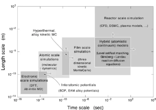
(12) CHAPTER 1 INTRODUCTION. 1.1 Motivation. 1.1.1 Multiscale Simulation in Materials Processing Vapor deposition (Fig. 1.1) is a multiscale process in the sense that growth of the film occurs in a reactor whose dimensions are of O (1m) for a time of O (102s), while the atomic assembly events involve length scales of O (10-10m) with time scales in the pico- to micro-second region. In fact, atomic assembly is more fundamentally determined by the making and breaking of chemical bonds which is described by the wave functions of bonding electrons with length and time scales of O (10-13m and 10-16s), respectively. Vapor deposition is not unique in this respect ─ all of materials science confronts a similar issue and many approaches have evolved for treating it [Ohno et al., 1999; Olson, 1997]. The ability to design processes for the growth of an atomic scale structure is critically tied to our ability to connect models with very disparate time and length scales. This ranges from the use of quantum mechanics to describe atomic binding to computational fluid dynamics (CFD) or direct simulation Monte Carlo (DSMC) [Bird, 1994] to account for complex flow fields, thermal gradients and reaction. 1.

(13) environments in the deposition chamber. This modeling hierarchy is summarized in Fig. 1.2. Some state-of-the-art modeling and simulation tools such as density functional theory (DFT), molecular dynamics (MD), kinetic Monte Carlo (kMC) and CFD when used alone enable analysis of only a part of a synthesis process. Among these, kMC method can be used to study the slow thermal diffusion of the deposited atoms/molecules on the substrate surface, which is important for predicting the correct morphology of the material structure. Energy barrier for atom jump at various atomic configurations on the substrate surface is required in the kMC method. However, it is very hard to obtain the data from experiment due to the difficulty of manipulating atom by atom precisely. Quantum computation considering large-scale atomic structure using DFT is the most possible and correct method to derive the data [Wadley et al., 2001].. 1.2 Background To describe completely the quantum mechanical behavior of electrons in solids it is strictly necessary to calculate the many-electron wave function for the system. In principle this may be obtained from the time-independent Schrödinger equation, but in practice the potential experienced by each electron is dictated by the behavior of all the other electrons in the solid. To solve the Schrödinger equation directly for all these. 2.

(14) electrons would thus require us to solve a system of around 1023 simultaneous differential equations. Such a calculation is beyond the capabilities of computers nowadays, and is likely to remain so for the foreseeable future. Evidently, we must involve some approximations to render the problem soluble albeit tricky. Here we have our simplest definition of DFT: A method of obtaining an approximate solution to the Schrödinger equation of a many-body system. For the past 30 years density functional theory has been the dominant method for the quantum mechanical simulation of periodic systems. In recent years it has also been adopted by quantum chemists and is now very widely used for the simulation of energy surfaces in molecules (Fig. 1.3). Either Schrödinger equation or DFT formulation are the eigenvalue problems. In the current thesis, we use the finite element method (FEM) to derive the matrix equation from DFT formulation and then use some efficient matrix solver to solve the eigenvalue (energy) and corresponding eigenvector. Advantages of using FEM for solving the DFT formulation include easier parallel implementation employing domain decomposition [Wu and Hsu, 2004] and possible mesh refinement in the regions where solution changes rapidly [Wu et al., 2004].. 3.

(15) 1.3 Literature Surveys. 1.3.1 Theoretical Development 1.3.1.1 Schrödinger equation The foundation of the theory of electronic structure of matter is the non-relativistic Schrödinger equation for the many-electron wave function Ψ [Schrödinger, 1926]. The much heavier nuclei are considered as fixed in space by the Born-Oppenheimer approximation, so the wave function Ψ depends on the position and spins of the N electrons [Michael, 2000]. 1.3.1.2 Hartree-Fock Theory Within Hartree-Fock theory one assumes the wave function of the N particle (electron) system to be an anti-symmetrized product of one particle (electron) functions [Markus, 2002]. Moreover, the HF is an approximation, as it does not account for dynamic correlation due to the rigid form of single determinant wave function. To account for dynamic correlation, one has to go to correlated methods, which use multi-determinant wave functions, and these scales as fifth, or even greater powers with the size of a system [Jan, 1996]. The calculation of the many-body wave function of a system of interacting electrons is a formidable task, which can only be carried out – and is only. 4.

(16) meaningful – for systems with a few tens of electrons [Kohn, 1999]. Its observables for larger systems are to be determined; the calculation of the many-body wave functions has to be avoided due to the seemingly formidable computational difficulty. 1.3.1.3 Hohenberg & Kohn Theorem In the year 1964 Hohenberg and Kohn published a paper in Physical Review, where they stated two fundamental theorems, which gave birth to modern density functional theory, an alternative approach to deal with the many body problem in electronic structure theory [Hohenberg and Kohn, 1964]. Up till now, both the exact ground state density as well as the Hohenberg-Kohn functional is still unknown, so one cannot make use of the Hohenberg-Kohn theorems to calculate the molecular properties. 1.3.1.4 Kohn-Sham Equations Kohn and Sham introduced a fictitious system of N non-interacting electrons to be described by a single determinant wave function in N “orbits” [Kohn and Sham, 1965]. The construction of the density explicitly from a set of orbits ensures that it is legal – it can be constructed from an asymmetric wave function. Due to the second part of the H&K theorem, namely that the total energy is minimized by the true ground-state density, the variational principle can now be utilized. With the standard functional. derivatives. and. the. additional 5. definition. of. the. so-called.

(17) exchange-correlation potential. The exchange-correlation functional ,εxc, which is simply the sum of the error made in using a non-interacting kinetic energy and the error made in treating the electron-electron interaction classically [Harrison]. All that remains now is the question what to do with theεxc, without which one cannot do any practical calculations. As mentioned above, this term has to tread on an approximate manner. Although there are many different functions available, almost all of them are derived from the electron density of a uniform electron gas, which can be calculated by means of statistical thermodynamics. 1.3.1.5 A New Density Functional Theory Formulation In a recent paper, a generic derivation from cluster expansion results in a new DFT formulation without the exchange-correlation term that makes the computation much traceable in physics without ad hoc assumption as mentioned in the above [Hsu, 2003].. 1.3.2 Numerical Methods In the past, numerical methods for solving DFT formulation can be divided into two categories. One is orbital-type method and the other is real-space method. The former includes computations using slater-type orbitals (STOs), Gaussian-type orbitals (GTOs) and plane waves, while the latter is the real-space method that can be. 6.

(18) loosely categorized as finite differences (FD), finite elements (FE), and wavelets. 1.3.2.1 Orbital-type method Linear combinations of analytical functions ϕ i (r ) = ∑ ciκ χ κ (r ) j. z. Plane Waves, χ κ (r ) = exp(ikκ r ). z. Slater Type Orbitals, χ κ (r ) = x kκ y lκ z mκ ⋅ exp(−ζ κ r ) , whose shape close to true orbits (hydrogen atom) but evaluation of integrals is expensive.. z. Gaussian Type Orbitals, χ κ (r ) = x kκ y lκ z mκ ⋅ exp(−ζ κ r 2 ) , whose evaluation of integrals cheap but different from true orbital shape.. Linear combination of GTOs to approximate STOs that is 1 STO ≈ 3 GTOs, but analytical integration is still much faster than with STOs (Fig. 1.4). 1.3.2.2 Real-space method. Real-space methods can loosely be categorized as one of three types: finite differences (FD), finite elements (FE), or wavelets. All three lead to structured, very sparse matrix representations of the underlying differential equations on meshes in real space. Applications of wavelets in electronic structure calculations have been thoroughly reviewed recently [Arias, 1999]. As implied in the title, the primary focus is on calculations in density functional theory (DFT); real-space methods are in no way limited to DFT, but since DFT calculations comprise a dominant theme in modern electrostatics and electronic structure, the discussion here will mainly be 7.

(19) restricted to this particular theoretical approach. The early development of FD and FE methods for solving partial differential equations stemmed from engineering problems involving complex geometries, where analytical approaches were not possible [Strang and Fix, 1973]. Example applications include structural mechanics and fluid dynamics in complicated geometries. However, even in the early days of quantum mechanics, attention was paid to FD numerical solutions of the Schrödinger equation [Kimball and Shortley, 1934; Pauling and Wilson, 1935]. Real-space calculations are performed on meshes; these meshes can be as simple as Cartesian grids or can be constructed to conform to the more demanding geometries arising in many applications. Finite-difference representations are most commonly constructed on regular Cartesian grids. They result from a Taylor series expansion of the desired function about the grid points. The advantages of FD methods lie in the simplicity of the representation and resulting ease of implementation in efficient solvers. Disadvantages are that the theory is not variational, and it is difficult to construct meshes flexible enough to conform to the physical geometry of many problems. Finite-element methods, on the other hand, have the advantages of significantly greater flexibility in the construction of the mesh and an underlying variational-type formulation. Other advantages include easier 8.

(20) parallel implementation using domain decomposition and possible mesh refinement in regions where solution changes rapidly, as mentioned earlier. However, the cost of the flexibility is an increase in complexity and more difficulty in the implementation of multiscale or related solution methods [Thomas, 2000].. 1.4 Objectives of the Thesis It is very attractive that this new DFT formulation can be solved without the uncertainty caused by the exchange-correlation term in principle. However, this DFT formulation is a typical eigenvalue problem, which is in principle more difficult to solve than a boundary-value problem from the numerical viewpoint. The design of the numerical scheme has to consider the future applications to system having a large numbers of electrons, which requires tremendous computing resources. In addition, the probability of electrons near the immobile ions (nucleus) often presents very large variations. Thus, in the current study we solve this new DFT formulation using finite element method, in which the advantages can be taken in the future for mesh refinement and parallelization using graph-partitioning technique (or domain decomposition). Therefore, the objectives of the current study are summarized as follows. 1.. To complete both 1-D and 3-D FE programs for solving the new DFT. 9.

(21) formulation. 2.. To apply the two programs to compute simple atomic (1 nucleus) systems, such as hydrogen atom (1 electron), helium-like atoms (2 electrons) and beryllium-like atoms (4 electrons).. 3.. To verify and compare the performance of 1-D and 3-D FE programs by comparing with available experimental data.. The thesis begins with descriptions of the FE method appropriate in the discreteness of 1-D and 3-D problems. Results of 1-D and 3-D computations are presented and discussed. Conclusions are then made in turn. Future development in this direction is also recommended at the end.. 10.

(22) CHAPTER 2 DENSITY FUNCTIONAL THEORY. 2.1 Ab-initio Methods. 2.1.1 Schrödinger Equation. The initial work on Density Functional Theory (DFT) was reported in two publications: the first with Pierre Hohenberg in 1964 and the next with Lu J. Sham in 1965. This was almost 40 years after E. Schrödinger [Schrödinger, 1926] published his first epoch-making paper marking the beginning of wave-mechanics. ⎛ 1 Za 1 ⎞⎟ +∑ Ψ =EΨ Schrödinger equation: ⎜ − ∑ ∇ 2 − ∑∑ ⎜ 2 i ⎟ i a ri − Ra i , j ri − r j ⎝ ⎠. (2.1). Where ri, rj are the positions of the electrons and Ra, Za are the positions and atomic numbers of the nuclei; and E is the energy. We will be primarily concerned with the calculation of the ground state energy of a collection of atoms. The energy may be computed by solution of the Schrödinger equation – which, in the time independent, non-relativistic, Born-Oppenheimer approximation is HΨ (r1 , r2 ,L, rN ) = EΨ (r1 , r2 ,L, rN ). (2.2). The wave function Ψ depends on the position and spins of the N electrons. The Hamiltonian operator, H, consists of a sum of three terms: the kinetic energy, the interaction with the external potential (Vext) and the electron-electron interaction (Vee). 11.

(23) That is N 1 N 2 1 H = − ∑ ∇ i + Vext + ∑ 2 i i < j ri − r j. (2.3). In materials simulation the external potential of interest is simply the interaction of the electrons with the atomic nuclei Vext = −∑∑ i. a. Za ri − Ra. (2.4). Note that in order to simplify the notation and to focus the discussion on the main features of DFT the spin coordinate is omitted here and throughout this article. The lowest energy eigenvalue, E0, is the ground state energy and the probability density of finding an electron with any particular set of coordinates {ri} is |Ψ0|2.. 2.1.2 Hartree Theory. One of the earliest attempts to solve the problem was made by Hartree. He simplified the problem by making an assumption about the form of the many-electron wave function, namely that it was just the product of a set of single-electron wave functions. Having made this assumption it was possible to proceed using the variational principle. In fact, for an N-electron system there are N equations for each of the N single-electron wave functions, which made up the many-electron product wave function [Stephen, 1997]. These equations turned out to look very much like the 12.

(24) time-independent Schrödinger equation, except the potential (the Hartree potential) was no longer coupled to the individual motions of all the other electrons, but instead depended simply upon the time-averaged electron distribution of the system. This important fact meant that it was possible to treat each electron separately as a single-particle. N r Ψ = ∏ϕ i (ri ). (2.5). i =1. where the ϕ i are orthonormal. Consequently the Hartree approximation allows us to calculate approximate single-particle wave functions for the electrons in crystals, and hence calculate other related properties. Unfortunately, the Hartree approximation does not provide us with particularly good results. The central failing of the Hartree approximation is that it does not recognize the Pauli exclusion principle. The true many-body wave function must vanish whenever two electrons occupy the same position, but the Hartree wave function cannot have this property. Mathematically, the Pauli exclusion principle can be accounted for by ensuring that the wave function of a set of identical fermions is anti-symmetric under exchange of any pair of particles. That is to say that the process of swapping any one of the fermions for any other of the fermions should leave the wave function unaltered except for a change of sign. Any wave function possessing that property will tend to zero (indicating zero probability) as any pair of fermions with the same quantum 13.

(25) numbers approaches each other. The Hartree product wave function is symmetric rather than anti-symmetric, so the Hartree approach effectively ignores the Pauli exclusion principle!. 2.1.3 Hartree-Fock Theory. The Hartree-Fock approach is an improvement over the Hartree theory in that the many-electron wave function is specially constructed out of single-electron wave functions in such a way as to be anti-symmetric. The wave function has to be much more complicated than the Hartree product wave function, but it can be written in a compact way as a so-called Slater determinant (for those who know what a determinant is). ΨHF =. Ψ=. 1 det[ϕ1ϕ 2ϕ 3 Lϕ N ] N!. ϕ1 (r1 ) ϕ1 (r2 ) L ϕ1 (rN ) 1 ϕ 2 (r1 ) ϕ 2 (r2 ) L ϕ 2 (rN ) N!. M M ϕ N (r1 ) ϕ N (r2 ) L ϕ N (rN ). (2.6). (2.7). Where the variables ri include the coordinates of space and spin. This simple ansatz for the wave function Ψ captures much of the physics required for accurate solutions of the Hamiltonian. Most importantly, the wave function is anti-symmetric with respect to an interchange of any two-electron positions. Ψ (r1 , r2 ,L ri , ri +1 ,L rN ) = −Ψ (r1 , r2 ,L ri +1 , ri ,L rN ) 14. (2.8).

(26) Starting from this assumption it is once again possible to derive the Hamiltonian equation for the system through the variational principle. Just as before, this results in a simple equation for each single-electron wave function. However, this time in addition to the Hartree potential (which described the direct Coulomb interaction between an electron and the average electron distribution) there is now a second type of potential influencing the electrons, namely the so-called exchange potential. The exchange potential arises as a direct consequence of including the Pauli exclusion principle through the use of an anti-symmetric wave function. Notably, the exchange potential contributes a binding energy for electrons in a neutral uniform system, so correcting one of the major failings of the Hartree theory. However, in calculating many other properties the Hartree-Fock approach is actually worse than the Hartree approach.. 2.1.4 Exchange-Correlation Energy. The reason the Hartree-Fock theory gives worse answers than the Hartree theory is simply that there is another piece of physics, which we are still ignoring. To some extent it cancels out with the exchange effect and so when we use the Hartree approach (i.e. we ignore both effects) we obtain reasonable results. On the other hand the Hartree-Fock approach includes the exchange effect but ignores the other effect,. 15.

(27) which balances it somewhat, completely. This new effect is the electrostatic correlation of electrons. Ignoring the Pauli exclusion principle generated exchange hole for the moment, we can also visualize a second type of hole in the electron distribution caused by simple electrostatic processes. If we consider the region immediately surrounding any electron (spin is now immaterial) then we should expect to see fewer electrons than the average, simply because of their electrostatic repulsion. Consequently each electron is surrounded by an electron-depleted region that known either the Coulomb hole (because of its origin in the electrostatic interaction) or the correlation hole (because of it origin in the correlated motion of the electrons). Just as in the case of the exchange hole the electron-depleted region is slightly positively charged. The effect of the correlation hole is twofold. Thus any other interaction effects, such as exchange, will tend to be reduced by the correlation hole [Stephen, 1997]. Clearly we can now see why the Hartree-Fock approach fails for solids: firstly the exchange interaction should be screened by the correlation hole rather than acting in full, and secondly the binding between the correlation hole and electron has been ignored. At this point, the Hartree-Fock approach gives quite creditable results for small molecules. This is because there are far fewer electrons involved than in a solid, and so correlation effects are minimal compared to exchange effects. 16.

(28) 2.1.5 Hohenberg & Kohn Theorem. The discussion above has established that direct solution of the Schrödinger equation is not currently feasible for systems of interest in condensed matter science – this is a major motivation for the development and use of density functional theory. DFT is based upon a fundamental observation that the total energy of an assembly of atoms is a function of the total electron charge density [Hohenberg and Kohn, 1964], which is a function of space and time. The electron density is used in DFT as the fundamental property unlike Hartree-Fock theory, which deals directly with the many-body wave function. Using the electron density significantly speeds up the calculation. Whereas the many-body electronic wave function is a function of 3N variables (the coordinates of all N atoms in the system) the electron density is only a function of x, y, z only three variables. In 1964 Hohenberg and Kohn proved the two theorems: 1.. For a non-degenerate ground state Ψ of the system the external potential Vext(r) is determined, within a trivial additive constant, as a functional of the electronic density n(r).. 2.. Given an external potential Vext(r), the correct ground-state density n(r) minimizes the ground-state energy E0, which is a functional uniquely determined by n(r). It holds, 17.

(29) E0 ≤ Ev [n~ ] where n~ (r) is any trial density fulfilling n~ (r ) ≥ 0 and. (2.9). ∫d. 3. r n~ (r ) = N , N being. the number of electrons in the system. They considered the ground state of the system to be defined by that electron density distribution which minimizes the total energy. Furthermore, they showed that all other ground state properties of the system (e.g. lattice constant, cohesive energy, etc) are functional of the ground state electron density. That is, that once the ground state electron density is known all other ground state properties follow (in principle, at least). The theorem – which has a remarkable short proof (Fig. 2.1) – guarantees the existence of an energy functional E[n] that reaches its minimum for the correct density n(r) yet gives no explicit prescription for its construction [Stephen, 1997]. In order to determine E[n] it is useful to separate the various known contributions to the total energy, like Ts[n], the kinetic energy of a non-interacting electron gas, Eext[n], the classical Coulomb energy of the electrons moving in the external potential Vext(r), and ECoul[n], the classical energy due to the mutual Coulomb interaction of the electrons: E [n(r )] = Ts [n(r )] + Eext [n(r )] + ECoul [n(r )] + E xc [n(r )]. (2.10). The last term Exc[n] contains the quantum-mechanical exchange and correlation energy and – in principle – the difference between the true kinetic energy, T[n], and 18.

(30) Ts[n], the kinetic energy of the gas of non-interacting Kohn-Sham electrons. But since this difference is very small it is typically neglected.. 2.1.6 Kohn-Sham Equations. Due to the second part of the H&K theorem, namely that the total energy is minimized by the true ground-state density, the variational principle can now be utilized. With the standard functional derivatives and the additional definition of the so-called exchange-correlation potential, v xc (r ) =. δE xc [n~ (r )] δ n~ (r ). (2.11). the following set of equations can be derived ⎡ 1 2 ⎤ ⎢⎣− 2 ∇ + veff (r )⎥⎦ϕ i (r ) = ε iϕ i (r ). (2.12). where the effective potential – as a functional of the electronic density – is given by veff = veff [n(r )] = vext (r ) + ∫ dr ′. n(r ′) + v xc [n(r )] r − r′. (2.13). and the electronic density as N. n( r ) = ∑ ϕ i ( r ). 2. (2.14). i =1. The set of equations (2.12) to (2.14) are the famous Kohn-Sham (KS) equations. They have to be solved self-consistently, i.e., starting from some initial density a potential veff [n(r)] is obtained for which the Eq. (2.12) are solved and a new electronic density Eq. (2.14) is determined. From the new density an updated effective potential can be. 19.

(31) calculated and this process is repeated until self-consistency is reached, i.e., until the new electronic density equals the previous one [Schöne]. In fact, the K-S equations give an exact description of the many-electron system since up to this point no approximations have been made. Nevertheless, the method has reasonable precision from the past experience. First-principle DFT methods can currently predict binding energies to within a tenth of an electron volt and bond lengths to within 0.02 Å. It is becoming relatively straightforward to use this method to analyze the kinetics of relevant surface processes, including adsorption, chemical reaction and diffusion. However, there exists an exchange-correlation functional Exc due to electrons in general DFT, which often requires some ad hoc assumptions (e.g., local density approximation (LDA) assuming uniform electron gas, [Seminario and Politzer, 1995]) to close the problem. The success of the density functional theory (DFT) in reproducing measurable physical quantities of many-electron systems is rather remarkable, and may be attributed to the very fact that in the configuration space where exists a density distribution that is unique, and corresponding to the lowest energy state, no matter how complex and populous the system might be. There are, however, physical properties that will require the phase space information, at the minimum the pair correlation in order to quantify the electron-electron interaction energy. 20.

(32) 2.2 Approximation to the Exchange-correlation Function The generation of approximations for Exc has lead to a large and still rapidly expanding field of research. There are now many different flavors of functional available which are more or less appropriate for any particular study.. 2.2.1 Local Density Approximation (LDA). The simplest, and at the same time remarkably serviceable, approximation for Exc[n(r)] is the so-called local density approximation (LDA). It is assumed that the density of an inhomogeneous system can be locally described by a homogeneous electron gas [Hohenberg and Kohn, 1964]. A homogeneous electron gas is fully specified by its electronic particle density n, which is often expressed in terms of the corresponding Wigner-Seitz radius rs, 1/ 3. ⎛ 3 ⎞ ⎟⎟ rs = ⎜⎜ ⎝ 4π n ⎠. (2.15). Within the LDA the functional for the exchange-correlation energy, Exc, can be written as E xc [n] = ∫ d 3 r [n(r )ε xc [n(r )]]. (2.16). where εxc is the exchange-correlation energy per particle of a homogeneous electron gas of density n. In the next step, the exchange-correlation potential is split into its exchange part vx and a correlation part vc, 21.

(33) v xc (rs ) = v x (rs ) + vc (rs ). (2.17). The local density approximation can be considered to be the zeroth order approximation to the semi-classical expansion of the density matrix in terms of the density and its derivatives [Dreizler and Gross, 1990].. 2.2.2 Generalized Gradient Approximation (GGA). In the generalized gradient approximation (GGA) a functional form is adopted which ensures the normalization condition and that the exchange hole is negative definite [Perdew and Wang, 1986]. This leads to an energy functional that depends on both the density and its gradient but retains the analytic properties of the exchange correlation hole inherent in the LDA. The typical form for a GGA functional is: E xc = ∫ d 3 r [n(r )ε xc (n(r ), ∇n(r ))]. (2.18). The GGA improves significantly on the LDA’s description of the binding energy of molecules – it was this feature which lead to the very wide spread acceptance of DFT in the chemistry community during the early 1990’s.. 2.3 New Density Functional Theory Formulation In a recent paper [Hsu, 2003], a generic derivation from cluster expansion results in a new DFT formulation (Eq. (2.21) as follows) without the exchange-correlation 22.

(34) term that makes the computation potentially much traceable in physics itself without any ad hoc assumptions. It was derived from the Schrödinger equation and reached a different form from the other DFT formulation. The wave function Ψ is chosen as the product of a single-electron wave function Φ, and an N-body correlation function, N. Ψ (Γ) = ∏ Φ (ri )U (Γ). (2.19). i =1. Γ is the N-particle phase space point equivalent to the expression (r1, r2, …, rn). The exchange symmetry is imposed on U and on the indistinguishable particles so that each electron is described by the same Φ. This gives the density function as follows: N. n(r ) = ∫ ∏ dτ i Φ (ri ) U (r1 , r2 ,K, rN )Φ (r ) ≡ Ψ0 (r ) 2. 2. 2. (2.20). i=2. where the index starting from i=2 is chosen for convenience by imposing the exchange symmetry, and dτi is the volume element of ith particle. The last derived equation is v. 1. v. I. ZI. 1 v 1 v v Ψ0 (r ) + ( N − 1)Ψ0 (r ) v v 2 r − r' r − RI. ε Ψ0 (r ) = − ∇ 2 Ψ0 (r ) − ∑ v 2. (2.21a). where. 1 r − r ′ = {∫ d 3 r ′ Ψ0 (r ′). 2. r − r′}. ∫d. 3. r ′ Ψ0 (r ′). 2. (2.21b). The subscript, I, refers to the immobile ion with charge ZI and N represents the number of electrons. This equation differs from the conventional DFT in several aspects. The usual exchange-correlation function disappears in this new formulation,. 23.

(35) while the electron-electron interaction differs by a factor 1 ( N − 1) . The derivation of 2. the density functional theory (DFT) from the cluster expansion corrects the spurious self-interaction energy in the ‘classical’ DFT, admits the excited states, and has a self-consistent exchange correlation effect.. 24.

(36) CHAPTER 3 NUMERICAL METHOD. The early development of FD and FE methods for solving partial differential equations stemmed from engineering problems involving complex geometries, where analytical approaches were not possible [Strang and Fix, 1973]. Example applications include structural mechanics and fluid dynamics in complicated geometries. However, even in the early days of quantum mechanics, attention was paid to FD numerical solutions of the Schrödinger equation [Kimball and Shortley, 1934, 10]. Real-space calculations [Thomas, 2000] are performed on meshes; these meshes can be as simple as Cartesian grids or can be constructed to conform to the more demanding geometries arising in many applications. Finite-difference representations are most commonly constructed on regular Cartesian grids. They result from a Taylor series expansion of the desired function about the grid points. The advantages of FD methods lie in the simplicity of the representation and resulting ease of implementation in efficient solvers. Disadvantages are that the theory is not variational, and it is difficult to construct meshes flexible enough to conform to the physical geometry of many problems. Finite-element methods, on the other hand, have the advantages of significantly greater flexibility in the construction of the mesh and an underlying variational formulation. In addition, parallel implementation using 25.

(37) domain decomposition, combining with adaptive mesh h-refinement, in FE methods due to unstructured mesh is rather straightforward by the use of graph-partitioning technique. The cost of these flexibilities may be an increase in complexity and more difficulty in the implementation.. 3.1 Finite Element Method (FEM) We begin with an introduction of the FEM that identifies the broad context of the subject [Burnett, 1987]: The FEM is the computer-aid mathematical technique for obtaining approximate numerical solution to the abstract of calculus that predict the response of physical system subjected to the external influences. Such problems arise in many areas of engineering, science, and applied mathematics. Applications to date have occurred principally in the areas of solid mechanics, heat transfer, fluid mechanics, and electromagnetism. New areas of application are continually being discovered, recent ones include solid-state physics and quantum mechanics. The salient features in FEM include the following:. 26.

(38) 1. The domain is divided into smaller regions called elements. Adjacent elements touch without overlapping, and there are no gaps between the elements. The shapes of the elements are intentionally made as simple as possible. 2. In each element the governing equations, usually in differential or variational (integral) form, are transformed into algebraic equation. The element equations are algebraically identical for all elements of the same type, which usually need to be derived for only one or two typical elements. 3. The resulting numbers are assembled (combined) into a much larger set of algebraic equations, which are called the system equations. In the process of element assembly, boundary conditions can be enforced automatically. Such huge systems of equations can be solved economically because the matrix of coefficients is “sparse” in essence. 4. Resulting matrix equation is then solved using suitable efficient matrix solver. ~ FEM seeks an approximate solution U , an explicit expression for U, in terms of. known functions, which approximately satisfies the governing equations and boundary conditions. It obtains an approximate solution by using the classical trial-solution procedure. Construction of a trial solution: ~ U ( x; a ) = a0 + a1 N1 ( x ) + a2 N 2 ( x ) + L + an N n (x ) 27. (3.1).

(39) where x are the independent variables in the problems. The functions N ( x ) are known functions called trial functions (basis). The coefficients, a, are undetermined parameters called degree of freedom (DOF). We apply FEM to solve the new DFT formulation, as shown in Eq. (2.21), which is a typical second-order nonlinear eigenvalue problem. The purpose is to determine specific numerical values for each of the parameters a. In this FEM, we employ Galerkin weighted residual method using C0-linear shape function. For each parameter ai we require that a weighted average of R(x;a) over the entire domain be zero. The weighting functions of the Galerkin weighted residual method are trial functions N ( x ) associated with each ai.. ∫ R(x; a )N (x )dx i. (3.2). 3.1.1 One-dimensional FEDFT Program. For the system of one nucleus with one or more electrons, Eq. (2.21) can be simplified as, by taking the spherical symmetry, 1 d2 Z ε ΨJ (r ) = − ΨJ (r ) − ΨJ (r ) + ΨJ (r )Π J (r ) 2 2 dr r. (3.3). where ΠJ = 0. ΠJ =. 1 HJ 2. for one-electron system (J=1). (3.4a). for two-electron system (J=1). (3.4b). 28.

(40) 1 ΠJ = HJ + HK 2. for four-electron system (J=1,2; K ≠ J) ∞. r. H J (r ) =. 1 r − r'. =. 2 2 1 dr ′ ΨJ( e ) (r ') r ′ 2 + ∫ dr ′ ΨJ( e ) (r ') r ′ ∫ r r ′= 0 r ′= r. J. (3.4c). ∞. ∫ dr ′ Ψ (r ') (e) J. 2. r′. (3.5). 2. r ′= 0. where ΨJ is the density function of orbital J that is limited to two electrons with spin polarization to satisfy the Pauli exclusion principle and ΨJ(e ) is the density function of the last evaluate. r is the radial coordinate originating from the center of the nucleus. By applying the Galerkin weighted residual to Eq. (3.3) in a typical 1-D element,. ∫∫∫ R(r; α )N (r ) dv = 0,. i = 1,2,..., n. i. (3.6). n. where N i (r ) is the shape function, Ψ(r ) ≈ U~(r;α ) = ∑α j N j (r ) and n is the number of j =1. nodes in an element. Note that the residual function, R(r;α), is defined as, R (r ;α ) = −. Z ~ 1 d2 ~ ~ ~ U J ( r ; α ) − U J ( r ; α ) + U J ( r ; α )Π J − ε U J ( r ; α ) 2 r 2 dr. (3.7). In the current study, linear shape function for 1-D element, Ni (rj ) = ai + bi rj = δ ij , is used for 1-D program throughout the research, unless otherwise specified. Note that the subscripts i and j are the node numbers in a 1-D element. Substituting Eq. (3.7) into Eq. (3.6), after some algebraic arrangement [Appendix A], results in the elemental generalized eigenvalue matrix (2x2) equation that its form is rearranged to satisfy the matrix solver as. { ε [M ] + [K ] }{α } = 0 29. (3.8).

(41) where. [K ] ij. [. [M ] = ⎡⎢ 15 b b r ij. ]. 1 ⎤ ⎡ 1 5 4 ⎢ − 5 bi b j Π J r + 4 Zbi b j − (ai b j + a j bi )Π J r + ⎥ ⎥ =⎢ ⎢ 1 ⎡ Z (a b + a b ) − 1 b b − a a Π ⎤ r 3 + Z a a r 2 ⎥ i j j i i j i j J ⎥ i j ⎥⎦ ⎢⎣ 3 ⎢⎣ 2 2 ⎦ i. ⎣. j. 5. +. 1 (ai b j + a j bi )r 4 + 1 ai a j r 3 ⎤⎥ 4 3 ⎦. (3.9a). (3.9b). Resulting system linear algebraic eigenvalue equations, obtained by assembling all elemental matrix equations as shown in Eq. (3.8), are then solved by the matrix solver by J-D method [Wang et al., 2003]. The stiffness matrix of the system equation resulting from the 1-D FEM is “marginally” diagonally dominant, from which the convergence is rather slow, which can be clearly shown in Fig. 4.17 ~ 4.18. For molecular system with more than one nucleus or with one nucleus and more than four electrons, the spherical symmetry is not held; hence, the three-dimensional FE program is required and is introduced next.. 3.1.2 Three-dimensional FEDFT Program. For the system of one nucleus with one or more electrons, Eq. (2.21) can be rewritten for density function of orbital J in three-dimensional form as, v. 1 2. v. Z r. v. v. v. ε ΨJ (r ) = − ∇ 2 ΨJ (r ) − v ΨJ (r ) + ΨJ (r )Π J ( r ). (3.10). where. v r = ( x, y , z ). (3.11a). 30.

(42) r = ( x 2 + y 2 + z 2 )1/ 2. (3.11b). v Π J (r ) : the same as Eq. (3.4). (3.11c). 2 v H J (r ) = 1 r − r ′ = {∫ d 3 r ′ ΨJ( e ) ( r ′) r − r ′ }. ∫d. 3. 2 v r ′ ΨJ( e ) ( r ′). (3.12). By applying the Galerkin FEM to Eq. (3.10) in a typical 3-D element, n v ~v v Ψ(r ) ≈ U (r ;α ) = ∑α j N j (r ) and n is the number of nodes in an element. Note that j =1. v N j (r ). v is the shape function in a typical 3-D element. Residual function, R( r ;α), is. then defined as, Z ~ v 1 ~ v ~ v ~ v v R ( r ; α ) = − ∇ 2U J ( r ; α ) − v U J ( r ; α ) + U J ( r ; α ) Π J − ε U J ( r ; α ) r 2. (3.13). In the current study, linear shape function for 3-D tetrahedral element, Nj =. a j + bj x + c j y + d j z 6Vc. , where Vc is the element volume, is used for 3-D program. throughout the research, unless otherwise specified. Similar to the algebraic rearrangement in 1-D FEM but comparably complicated [Appendix B], the resulting elemental generalized eigenvalue matrix (4x4) equation can be written as. { ε [M ] + [K ] }{α } = 0. (3.14). where. [M ] = VT. i = j , T = 10 ; i ≠ j , T = 20. c. ij. [K ] = A ij. ij. Aij = − Bij =. + Bij + C ij. (3.15a) (3.15b). bi b j + ci c j + di d j. (3.15c). 72Vc. n (a + b x + c y + d z )(a + b x + c y + d z ) Z i i k i k i k j j k j k j k ⋅∑ wk 2 2 2 36Vc k =1 xk + y k + z k. 31. (3.15d).

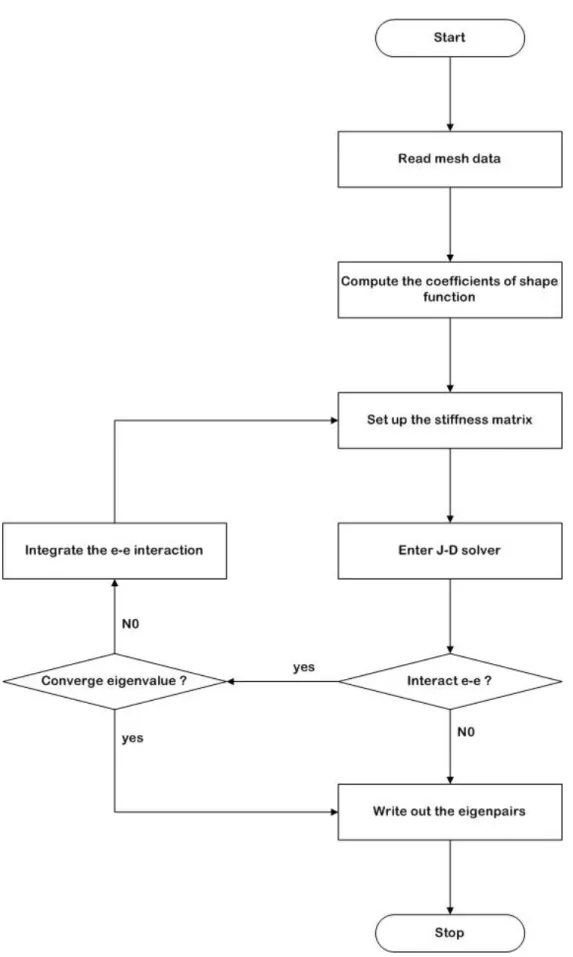
(43) C ij = −. Vc ΠJ T. i = j , T = 10 ; i ≠ j , T = 20. (3.15e). (e) v 2 v ΨJ (r ′) ∫∫∫ d r ′ rv − rv′ α = ≡ 3v (e) v 2 β ′ ′ ( ) d r r Ψ J ∫∫∫ 3. v H J (r ) =. α=. tot .element. ∑ 1. β=. 1 v v r −r′. ⎡ Gauss points ⎢V ⎢ c ∑ k =1 ⎣. tot .element. ∑ 1. J. (3.16a). v 2 ΨJ( e ) (rk '). (x. − x k ) + ( y j − y k ) + (z j − z k ) 2. j. 2. ⎡ Gauss points ( e ) v 2 ⎤ ⎢Vc ∑ ΨJ (rk ') wk ⎥ k =1 ⎦ ⎣. 2. ⎤ wk ⎥ ⎥ ⎦. (3.16b). (3.16c). Note that Gauss Quadrature [Zienkiewicz and Taylor, 2000] with weighting factor wk at point k is used for the volume integration throughout the study, unless otherwise specified. This generalized eigenvalue formulation can be easily extended to more complicated atomic or molecular system (multiple orbits) by modifying the electron-electron interaction term, Π j (r ) , based on the Pauli exclusion principle. Resulting system equations are then assembled element by element and are solved by using J-D matrix solver similar to 1-D FE program. However, the convergence of the 3-D FE program is expected to be much faster than that in 1-D FE program due to the diagonally dominated coefficient matrix, which can be shown in Fig. 4.17 ~ 4.18. The system equations are an eigenvalue problem with large-scale sparse matrix. Here we use the method of random pack storage (RPS) to just store the nonzero entries of the stiffness matrix. This method can save a lot of memories when store a large-scale sparse matrix. Resulting eigenvalue linear algebraic equations are then. 32.

(44) solved using the Jacobi-Davison (JD) method [Wang et al., 2003], which is a subspace-type algorithm that will be introduced shortly. Overall procedures of solving the DFT eigenvalue problem can be schematically sketched in Fig. 3.1.. 3.2 Jacobi-Davidson Method The Jacobi-Davidson method [Voss and Betcke, 2002; Hwang, 2003] is based on a combination of two basic principles. The first one is to apply a Galerkin approach for the eigenproblem Ax = λx , with respect to some given subspace spanned by an orthonormal basis {v1, …, vm}. The Galerkin condition is. AVm s − θVm s ⊥ {v1 ,K, vm }. Vm* AVm s − θ s = 0. (3.17). where Vm denotes the matrix with columns v1 to vm. This equation has m solutions. (θ. (m) j. ). (. ). , s (jm ) . The m pairs θ j( m ) , u (jm ) ≡ Vm s (jm ) are called the Ritz values and Ritz. vectors of A with respect to the subspace spanned by the columns of Vm. These Ritz pairs are approximations for eigenpairs of A, and our goal is to obtain better approximations by a well-chosen expansion of the subspace. Suppose that we have an eigenvector approximation uj for an eigenvector x corresponding to a given eigenvalue λ. We suggested computing the orthogonal correction t for uj(m). A(u (jm ) + t ) = λ (u (jm ) + t ). 33. (3.18).

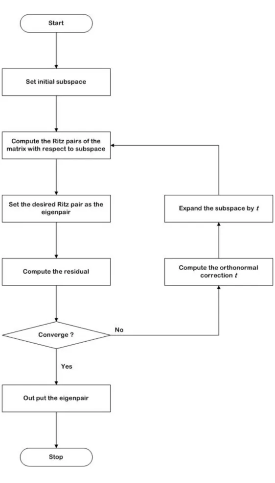
(45) ) ⊥ with t ⊥ u (m ≡ {v | v *u j = 0} . j , t ∈U. The correction equation of Jacobi-Davidson. (A. ⊥. ). − θ j I t = −rj. (3.19). where rj = ( A − θ j I ) u j. (3.20a). A ⊥ = (I − u j u *j ) A(I − u j u *j ). (3.20b). The next is to solve the t from Eq. (3.19) and add t into subspace to expand the search subspace, then iterate again with expansive subspace until convergence. The Jacobi-Davidson method has similar convergence properties as inverse iteration if the correction equation is solved exactly. Procedures of solving eigenvalue problem using J-D algorithm can shown in Fig. 3.2, while the details are summarized as follows [Wang et al., 2003]: 1.. Given A(λ ) = λA1 + A0. 2.. To choose a random vector Vi as the initial subspace. 3.. * To compute the Galerkin condition as M i= V AiV .. 4.. To compute the Ritz pairs (θ , s ) of (θ M 1 + M 0 ) s = 0 and select the desired Ritz pair to be eigenpair with s. 2. = 1.. 5.. To compute u = Vs , and the residual r = A(θ )u .. 6.. If. (r. 2. ). < ε , λ =θ,. x = u , Quit. 34.

(46) 7.. To compute correction term t and orthogonalize t against V, v = t / t. 8.. Expand V = [V , v ]. 9.. To back to process 3 and iterate until r 2 < ε .. 2. This J-D solver can efficiently deal with the large-scale sparse eigenvalue matrix equation, which is still a very challenging task even nowadays. One of the advantages in using J-D algorithm to solve the DFT eigenvalue problem is the feasibility of parallelization in the future, considering the computational demanding of the problem itself.. 35.

(47) CHAPTER 4 RESULTS AND DISCUSSIONS. In this chapter, we first describe the elements of different cases and different computational domains and then several computational results are presented in turn.. 4.1 Elements Construction We set up two different dimensions of elements to fit the different FEDFT programs.. 4.1.1 One-dimensional Elements. Since the simple atoms that only need to consider the s state of the angular momentum are spherical symmetry, we could simplify the computational domain of sphere to be just the radial domain. We have to set up the one-dimensional elements to match the one-dimensional FEDFT program in the radial domain. The computing radii are different for different cases (ex. the hydrogen atom is about 10 for ground state and about 20 for first excited state) but the length unit is Bohr radius, a0, (0.053 nm). The domain is formed by nodes and elements that two nodes compose one element in one-dimensional domain. The Fig.4.1 shows the diagram of the elements and nodes and the radial domain data of all models in this research are shown in table 4.1. 36.

(48) 4.1.2 Three-dimensional Elements. The radial domain is only suitable for the simple atoms. When the models are many electron atoms that have to consider the other angular momentums, molecules and cluster of atoms etc. are complicated, we will have to solve the complicated problems. and. need. the. total. real-space. computational. domain.. In. the. three-dimensional elements, we use the tetrahedron as an element that is used for 3-D program throughout the research, unless otherwise specified and there are four nodes to compose one linear element (Fig.4.2). In the case of simple atoms, we cut part of a sphere to simplify the computational domain and decrease the computing time. For example the hydrogen atom, we set the radius to be 10 Bohr radii and both the zenith and azimuth angle to be 30 degrees as shown in Fig. 4.3. There are 60 nodes on the radial and 20 nodes both on the zenith and azimuth angle. The computational domain data of all models in this research are shown in table 4.2.. 4.2 One-dimensional FEDFT We take the hydrogen atom, helium-like atoms and beryllium-like atoms as models to validate the one-dimensional FEDFT program. The 1s state energies and 2s state energies of all models obtained by one-dimensional FEDFT program that are. 37.

(49) compared with the known experimental ones and numerical ones obtained by Hsu [Hsu, 2003] are shown in table 4.3 - 4.5. The numerical energies obtained by Hsu are obtained by finite difference method (FDM). The Z column shows the numbers of positive charge of the nucleus. The exp column shows the ionization energy of the electron from experiments. The n=1 column shows the 1s state energy of the electron from numerical results. The n=2 column shows the 2s state energy of the electron from numerical results. The subscripts F and H mean the numerical results by FEDFT and Hsu. The models set the different cutoff radii that all are divided by 0.001 Bohr radii as an element. Since there are four electrons in beryllium-like atoms, the ground state energy, G, is the sum of 1s and 2s state energies. From the table 4.3, the numerical ground state energy of hydrogen atom almost conforms to the experiment. It shows that the one-dimensional FEDFT program has good performance to compute the energy of hydrogen atom. But the table 4.4 and 4.5 show that the numerical results of both FEDFT and FDM do not conforms to the experiments closely. The reason should be the electron-electron interaction term that can not directly be solved by the initial equation but integrates by the last eigenvectors. The results of FEDFT are worse than FDM shown in table 4.4 and 4.5. When in one-dimensional, the matrices of both FEDFT and FDM are tri-diagonal matrices. In the current research, the stiffness matrix of the one-dimensional FEDFT is 38.

(50) “marginally” diagonally dominant, and it would obtain the worse solution and converge slowly. The probabilities of finding the electron in a hydrogen atom for the 1s and 2s states that are compared with exact solutions are shown in Fig. 4.4. The probabilities of finding the electron in helium-like atoms for the 1s and 2s state are shown in Fig. 4.5 ~ 4.9 and the comparisons of the probabilities of finding the electron in helium-like atoms for the 1s and 2s state are shown in Fig. 4.10 and 4.11. The probabilities of finding the electron in beryllium-like atoms for the 1s and 2s state are shown in Fig. 4.12 ~ 4.14 and the comparisons of the probabilities of finding the electron in helium-like atoms for the 1s and 2s state are shown in Fig. 4.15. Fig. 16 shows the photographic representation of the electron probability-density distribution and the numerical results conform to them.. 4.3 Three-dimensional FEDFT To solve the complicated models, we construct the three-dimensional FEDFT program. To validate the three-dimensional FEDFT program, we take the hydrogen and helium atoms to be test models. The cutoff radius is 20 Bohr radii divided by 300 nodes in radial direction, and both the zenith and azimuth angle are 30 degrees divided by 20 nodes in all angular directions for hydrogen atom model, and there are. 39.

(51) total 165150 nodes and 796588 elements in this computational domain. The cutoff radius is 5 Bohr radii divided by 50 nodes in radial direction, and both the zenith and azimuth angle are 15 degrees divided by 15 nodes in all angular directions for helium atom model, and there are total 3668 nodes and 14629 elements in this computational domain. The numerical energies of hydrogen and helium atoms are shown in table 4.6 and 4.7. The subscripts 1d and 3d mean the numerical results obtained by one-dimensional and three-dimensional FEDFT, and H means the numerical results by Hsu. Note that the three-dimensional ground state energy of helium atom with electron-electron interactions is a temporal solution. The numerical ground state energy of hydrogen atom almost conforms to the experiment and the three-dimensional numerical results also conform to the one-dimensional. numerical. ones.. Although. the. one-dimensional. and. three-dimensional FEDFT both obtain the good approximation, the rate of convergence of three-dimensional FEDFT is much quicker than the one of one-dimensional FEDFT for hydrogen atom model that are shown in Fig. 4.17 ~ 4.18. Obviously, there are a lot of jumps in the convergence of one-dimensional FEDFT but it almost converges directly by three-dimensional FEDFT, mainly due to the strong diagonal dominance of the stiffness matrix in the three-dimensional FEDFT. From table 4.7, the numerical ground state energy of helium atom obtained by 40.

(52) three-dimensional FEDFT has a better approximation than those obtained by Hsu and one-dimensional FEDFT. It is probably due to the strong diagonal dominance of the stiffness matrix in the three-dimensional FE formulation. To compare the solutions of two kinds of FEDFT, the FEM has better performance for three-dimensional model than one-dimensional model. The probabilities of finding the electron in a hydrogen atom for the 1s and 2s states that are compared with exact solutions are shown in Fig. 4.19. The probability of finding the electron in a helium atom for the 1s state that is compared with one-dimensional FEDFT is shown in Fig. 4.20.. 41.

(53) CHAPTER 5 CONCLUSIONS. In the current study, the approximations of new density-functional-theory formulation with different atoms obtained by one-dimensional and three-dimensional finite element methods that the eigenpairs of the stiffness matrices solved by Jacobi-Davidson method are presented. The major findings of the current research are summarized as follows: 1. The method of random-pack-storage that only records the value of the nonzero entries of matrices reduces the storage space of memory substantially and can avoid the problem of the large-scale sparse matrix that needs a lot of space to record all entries. 2. The matrix solver of Jacobi-Davidson method has good performance to compute the desired eigenpair of large-scale sparse matrices in an eigenproblem. It can solve rather efficiently the stiffness matrix derived from finite element method. 3. The Gauss Quadrature is a powerful numerical integration that can simplify a complicated integral and obtain a very good approximation. 4. For the same size of elements, the larger cutoff radius is, the better approximation is. 5. For hydrogen atom, the one-dimensional and three-dimensional FEDFT programs 42.

(54) both have good approximations of the 1s and 2s state energies. 6. The solutions of one-dimensional finite element method are worse than those of one-dimensional finite difference method for the new density-functional-theory formulation probably due to the marginally diagonal dominance of the stiffness matrix in the 1-D FE formulation. 7. Convergence rates of three-dimensional FEDFT are much faster than those of one-dimensional FEDFT, mainly due to the strong diagonal dominance of the stiffness matrix in the 3-D FE formulation. 8. For helium atom, the three-dimensional FEDFT obtains a better solution than one-dimensional FEDFT.. 43.

(55) CHAPTER 6 FUTURE WORKS. From this study, future work is summarized as follows: 1. To confirm the three-dimensional FEDFT program that computes the helium-like and beryllium-like atoms successfully. 2. To compute the hydrogen molecule that is a two nuclei and two electrons system by the three-dimensional FEDFT program. 3. To compute the carbon atom that is a one nucleus and six electrons system and it has to consider the 2p orbit. 4. If the serial code performs correctly, we will parallelize it to improve the efficiency and to solve more complicated cases.. 44.

(56) REFERENCES 1. Arias, T. A. (1999), Multiresolution analysis of electronic structure: semicardinal and wavelet bases, Rev. Mod. Phys., 71:267. 2. Arthur Beiser (1995), Concepts of Modern Physics, McGraw-Hill, New York, 216-217. 3. Bird, G..A. (1994), Molecular Gas Dynamics and The Direct Simulation of Gas Flows, Oxford University Press Inc., New York. 4. Burnett, David S. (1987), Finite Element Analysis from Concepts to Applications……. 5. Dreizler, R. M. and Gross, E. K. U. (1990), Density Functional Theory, Springer Verlag, Berlin. 6. Friedrich, C., Fritz Haber-Institut der Max-Planck-Gesellschaft, Berlin. 7. Harrison, N. M., An Introduction to Density Functional Theory. 8. Hohenberg, P. and Kohn, W. (1964), Phys Rev B, 136:864. 9. Hsu, J.Y. (2003), Derivation of the Density Functional Theory from the Cluster Expansion, Phys. Rev. Lett., 91:133001. 10. Hwang, T.M. (2003), Numerical experiences of large-scale eigenvalue problems with Jacobi-Davidson method. 11. Jan K. Labanowski (1996), Simplified and Biased Introduction to Density Functional Approaches in Chemistry. 12. Kimball, G. E., and Shortley, G. H. (1934), Phys. Rev., 45:815. 13. Kohn, W and Sham, L.J. (1965), Phys Rev A, 140:1133. 14. Kohn, W. (1999), Electronic structure of matter—wave functions and density functionals, Rev. Mod. Phys., 71:1253. 15. Markus Oppel (2002), DFT – Density functional theory. 16. Michael P. Marder. (2000), Condensed matter physics. 17. Ohno, K., Esfarjani, K., and Kawazoe, Y. (1999), computational materials science (from ab-initio to Monte Carlo methods). Springer-Verlag, Berlin. 18. Olson, G.B. (1997), Science; 277:1237. 19. Pauling, L., and Wilson, E. B. (1935), Introduction to Quantum Mechanics, Dover, New York, p. 202. 20. Perdew, J. P. and Wang, Y. (1986), Phys. Rev. B 33, 8800; Ibid. E 34, 7406. 21. Schöne, Wolf-Dieter, Density-functional theory and the Kohn-Sham equations. 22. Schrödinger, E. (1926), Am. Physik 79, 361. 23. Seminario, J.M., and Politzer, P. ed. (1995), Modern Density Functional Theory: A Tool for Chemistry, Elsevier. 24. Stephen Jenkins (1997), The Many Body Problem and Density Functional 45.

(57) 25. 26. 27. 28.. 29.. 30.. 31.. 32.. Theory, http://newton.ex.ac.uk/research/semiconductors/theory/people/jenkins/mbody/m body3.html . Strang, G., and Fix, G. J. (1973), An Analysis of the Finite Element Method, Prentice-Hall, Englewood Cliffs. Thomas L. Beck (2000), Real-space mesh techniques in density functional theory, Reviews of Modern Physics. Voss, H. and Betcke, T. (2002), A Jacobi-Davidson-type projection method for nonlinear eigenvalue problems, preprint submitted to Elsevier Science. Wadley, H.N.G., Zhou, X., Johnson R.A., and Neurock, M. (2001), Mechanisms, models and methods of vapor deposition, Progress in Materials Science, 46:329-377. Wang, W., Hwang, T.-M. Lin, W.-W. and Liu, J.-L. (2003), Numerical methods for semiconductor heterostructures with band nonparabolicity, J. Comp. Phys., 190:141-158. Wu, J.-S. and Hsu, K.-H. (2004), Progress Twoards Parallel Particle Modeling of DC-Magnetron Sputtering Plasma, 24th International Symposium on Rarefied Gas Dynamics, July 10-16, 2004, Bari, Italy. Wu, J.-S., Tseng, K.-C. and Wu, F.-Y. (2004), Parallel Three-Dimensional DSMC Method Using Mesh Refinement and Variable Time-Step Scheme, Computer Physics Communications (accept). Zienkiewicz, O.C. and Taylor, R.L. (2000), The Finite Element Method: The Basis, Butterworth-Heinemann, 219-223.. 46.