無線區域網路即時性資料傳輸品質保證之動態調整競爭性通道存取資料參數

國 立 交 通 大 學

電信工程學系

碩 士 論 文

無線區域網路即時性資料傳輸品質保證之

動態調整競爭性通道存取資料參數

Dynamically Control Data Parameter for Protecting

Real-Time Transmissions in IEEE 802.11e EDCA

研究生： 陳偉志

指導教授： 李程輝 教授

動態調整競爭性通道存取資料參數

研 究 生： 陳偉志

_{Student: Wei-Chih Chen}

指導教授： 李程輝 教授

_{Advisor: Prof. Tsern-Huei Lee}

國 立 交 通 大 學

電 信 工 程 學 系 碩 士 班

碩 士 論 文

A Thesis

Submitted to Institute of Communication Engineering College of Electrical Engineering and Computer Science

National Chiao Tung University in Partial Fulfillment of the Requirements

for the Degree of Master of Science

in

Communication Engineering June 2005

Hsinchu, Taiwan, Republic of China.

動態調整競爭性通道存取資料參數

研究生： 陳偉志

指導教授： 李程輝 教授

國立交通大學

電信工程學系碩士班

中文摘要

隨著無線區域網路快速地普及，近來提升無線網路的能力越來越引人注意， 目的在於提供較嚴格的服務品質保證(QoS)給即時資料傳輸。在本論文的探討 中，我們評估新的 IEEE 802.11e 標準中所用來支援服務品質保證的機制，也就是 在原本 IEEE 802.11 標準中的媒介存取控制層(MAC)，定義新的加強媒介存取控 制層機制來提供服務品質保證。我們發現該標準中的機制 EDCA 可以藉由不同 的存取分類(Access Category)提供令人滿意的差別服務。然而，在傳輸負載過多 的狀況下，對於即時資料的傳送，EDCA 並不能提供有效的服務品質保證。因此， 我們提出盡力式資料(best-effort data)的控制以及允入控制(admission control)等機 制，希望在高網路負載的情況下，對於即時資料的傳輸，EDCA 依然能夠提供較 佳的服務品質保證。主要的觀念是將即時資料傳送(real-time transmission)以及盡 力式資料傳送(best-effort transmission)分開處理。擷取點(access point)根據網路的 傳輸狀況，幫助工作站(station)判斷決定接受或拒絕即時資料的傳送和動態地控 制盡力式資料傳送以保護正在傳送的即時資料。經由模擬驗證，我們證實了該機 制在高負載狀況下能夠發揮功效。

Real-Time Transmissions in IEEE 802.11e EDCA

Student: Wei-Chih Chen

Advisor: Prof. Tsern-Huei Lee

Institute of Communication Engineering

National Chiao-Tung University

Abstract

With the fast deployment of wireless local area networks (WLANs), the ability of WLAN to support real time services with stringent quality of service requirements has come to the fore. In the thesis, we evaluate the capability of QoS support in the IEEE 802.11e standard, which is the medium access control (MAC) enhancement for QoS support in IEEE 802.11 standard. We find that EDCA provides satisfactory service differentiation among its different access categories. However, in the case of heavy load traffic, the QoS of real-time traffic can not be assured. Thus, we proposed best-effort data control and admission control schemes that enable EDCA to provide quantitative bandwidth guarantees. Real-time transmissions and best-effort data transmissions are handled differently. The access point (AP) helps stations make decisions on acceptance or rejection of real-time traffic and dynamically control the data parameters to protect the existing real-time traffic according to the network condition. Simulation results confirm the effectiveness of the proposed methods.

Acknowledgements

Deeply thank to my advisor, Professor Tsern-Huei Lee, for his continuous encouragement, support, and enthusiastic discussion throughout this research. His valuable suggestions help me to the success of this work.

Also I would like to thank the members of network technologies laboratory in the Institute of Communication Engineering, National Chiao Tung University, for their stimulating discussion and help.

This thesis is dedicated to my parents for their patience, love, encouragement and long expectation. At last, thank all my friends who support and concern me so far.

中文摘要 i

English Abstract ii

Acknowledgements iii

Contents iv

List of Figures vi

List of Tables viii

Chapter 1 Introduction 1

Chapter 2 Backgrounds 3

2.1 An over view of IEEE 802.11 WLAN... 3

2.1.1 A brief of IEEE 802.11 standard... 3

2.1.2 The IEEE 802.11 MAC…………... 4

2.1.3 Distributed Coordination Function, DCF... 5

2.1.3 Point Coordination Function, PCF... 8

2.2 IEEE 802.11e QoS Enhancement Standard... 9

2.2.1 A brief of IEEE 802.11e standard... 9

2.2.2 Enhanced Distributed Channel Access, EDCA... 10

2.2.3 HCF Controlled Channel Access, HCCA……... 13

3.1 Related Work………... 17

3.1.1 Possible Performance Improvement in MAC Layer... 17

3.1.2 Protocol Model and Performance Analysis of EDCA... 19

3.1.3 Adaptive EDCF, AEDCF………... 22

3.2 Proposed Methods………... 24

Chapter 4 Performance Evaluation 33 4.1 Simulation Scenario………... 33

4.2 Priority Test……….………... 34

4.3 Simulation Results for DCF and EDCA………... 36

4.4 Simulation Results for the Proposed Method………... 40

Chapter 5 Conclusion 45

2.1 Standards of IEEE 802.11 MAC and PHY layers………... 4

2.2 The IEEE 802.11 MAC Architecture………….………. 5

2.3 Basic DCF CSMA/CA Scheme……….………. 6

2.4 RTS/CTS Access Scheme……..………. 7

2.5 PCF and DCF Cycles………... 8

2.6 Diagram of IEEE 802.11e Architecture….………. 9

2.7 DCF and EDCA Comparison………..…... 11

2.8 The Timing Diagram of EDCA……….……….. 12

2.9 A Typical HCF Beacon Interval………..… 14

2.10 An Example of Scheduler for Streams from QSTA “i” to “k” ……... 16

3.1 Markov Chain Model of EDCA………...… 22

3.2 The Calculation of Transmission Budget……….……… 27

3.3 An Example of Utilizing the Transmission Budget…...……….. 28

3.4 The Diagram of STT, STT, and Idle...………. 29

3.5 The Control Mechanism at the t -th Interval..……….... 30

4.1 Simulation Topology………...………. 33

4.4 The Throughput for DCF………. 37

4.5 The Throughput for EDCA……….. 37

4.6 The Mean Latency for DCF……….……… 38

4.7 The Mean Latency for EDCA……….……… 38

4.8 The Throughput for EDCA at High Loads ………... 39

4.9 The Mean Latency for EDCA at High Loads………...………... 39

4.10 The Throughput of EDCA without Protecting Real-Time Traffic…... 40

4.11 The Mean Latency of EDCA without Protecting Real-Time Traffic... 41

4.12 The Throughput of EDCA with Protecting Real-Time Traffic…..….. 41

4.13 The Mean Latency of EDCA with Protecting Real-Time Traffic…… 42

4.14 The Throughput of EDCA without Data Control……… 43

4.15 The Mean Latency of EDCA without Data Control……… 43

4.16 The Throughput of EDCA with Data Control………. 44

2.1 Mapping of IEEE 802.1D User Priority to Access Category……….. 10 2.2 The Default EDCA Parameter Set………..…. 12 4.1 The IEEE 802.11a PHY/MAC parameters…..……… 33 4.2 MAC Parameters for the Three Traffic Categories….………. 34

Chapter 1

Introduction

The past few years have seen an explosion in the deployment of wireless networks conforming to the IEEE 802.11 standard [1]. Consumers require more convenient and powerful wireless technology to facilitate the QoS of the online chatting or videoconference, etc. Therefore, the IEEE 802.11e group is developing MAC improvements to support QoS applications to make more efficient use of the wireless channel.

The original IEEE 802.11 MAC protocol included two modes of operation characterized by coordination functions: DCF and PCF. The IEEE 802.11e draft [2] mainly concerns the MAC layer protocol, which introducing new EDCA and HCCA mechanisms. That means the modification is only in the MAC layer and it can provide different service quality for traffic streams with different priorities. Many works, [3], [4], [5] and [6], have been done. However, the main focus was on studying the EDCA differentiated mechanisms. Traffic belonging to a higher priority class has a higher probability of transmission, thus achieving a higher throughput when competing with lower priority traffic. But, no guarantee of higher priority traffic in terms of throughput and delay performance is given since the spirit of the IEEE 802.11e is also based on contention based access mechanisms.

In this thesis, we proposed an admission control scheme to protect existing real time traffic at high network loads. With this scheme, we can provide guaranteed throughput of real time traffic. With comparing with the HCCA mechanism, the

scheme is easier to be implemented on QAP and QSTA. Then, simulation results demonstrate the practicable to protect the existing traffic and manage the resources effectively according the network condition.

The remainder of the thesis is organized as follows. We briefly introduce the mechanisms of the IEEE 802.11 standard and the IEEE 802.11e standard in Chapter2. In Chapter 3, we will review some possible improvements on performance and discuss our proposed methods. We evaluate the proposed algorithm with extensive simulations in Chapter 4. Finally, Chapter 5 concludes the thesis.

Chapter 2

Backgrounds

2.1 An overview of IEEE 802.11 WLAN

2.1.1 A brief of IEEE 802.11 standard

The IEEE 802.11 WLAN standard defines the Media Access Control (MAC) layer and the Physical (PHY) layer of the open system interconnection (OSI) network reference model. Fig. 2.1 shows different standards done at IEEE 802.11 MAC and PHY layers. IEEE provides three kinds of options in the PHY layer to support data transmission up to 2 Mbps at 2.4GHz. These options are a frequency hopping spread spectrum (FHSS) radio, a direct sequence spread spectrum (DSSS) radio, and an infrared (IR) baseband PHY, respectively. As going by the demand of higher data transmission rate, the IEEE defines two high rate extensions: the IEEE 802.11b and the IEEE 802.11a. The IEEE 802.11b standard, based on DSSS technology, is in the 2.4GHz band with data rates up to 11Mbps and the IEEE 802.11a standard, based on orthogonal frequency division multiplexing (OFDM) technology, is in the 5GHz band with data rates up to 54Mbps. Recently, the IEEE 802.11g is finalized which extends the IEEE 802.11b PHY layer to support data rates up to 54Mbps in the 2.4GHz band. Further enhancement on these standards is still on-going.

Fig. 2.1 Standards of IEEE 802.11 MAC and PHY layers [7]

To enhance the quality of service (QoS) performance of IEEE 802.11 WLAN, the IEEE 802.11e is developed. In the IEEE 802.11f, the standard defines an Inter-Access Point protocol to allow STAs roaming between muti-vendor access points. Lastly, the IEEE 802.11i standard is to enhance security and authentication mechanisms for IEEE 802.11 MAC.

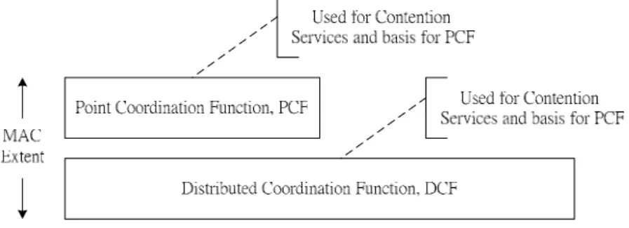
2.1.2 The IEEE 802.11 MAC

The IEEE 802.11 MAC protocol defines two access methods, the basic Distributed Coordination Function (DCF) and the optional Point Coordination Function (PCF). While the DCF is responsible for asynchronous data services, the PCF was developed for time-bounded services. The IEEE 802.11 can operate both in contention-based DCF mode and contention-free PCF mode. The implementation of DCF is mandatory in all IEEE 802.11 stations, but the implementation of PCF which basically implements a polling-based access is not mandatory. The reason is that the hardware implementation of PCF is too complex and there are some unsolved problems, like unpredictable beacon delays and unknown transmission durations of

the polled stations [8]. The basic MAC architecture is illustrated in Fig. 2.2.

Fig. 2.2 The IEEE 802.11 MAC Architecture

2.1.3 Distributed Coordination Function, DCF

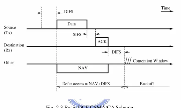
DCF access method adopts carrier sense multiple access with collision avoidance (CSMA/CA) mechanism to provide services for data transmission. It guarantees the fairness and distribution character among wireless stations. In this mode, a station must sense the medium before initiating a packet transmission. If the medium is sensed as being idle for a time interval longer than a Distributed InterFrame Space (DIFS), then the station can transmit the packet immediately. At the same time, other stations defer their transmission while adjusting their network allocation vectors (NAVs) and then start the backoff procedure, as shown in Fig. 2.3. In this procedure, the station computes a random time interval, called backoff timer, uniformly distributed between zero and maximum called Contention Window (CW). The backoff timer function is defined in equation (2.1), where CW_min <CW <CW_max and

time

slot _ depends on the different physical layer type. The backoff timer is

decreased when the medium is idle and frozen when another station is transmitting. backoff timer =rand

[

0,CW

]

⋅slot_time (2.1) Specifically, each time the medium becomes idle, the station waits for a DIFS and periodically decrements the backoff timer until it expires. Once the backoff timer

counts down to zero, the station is authorized to access the medium. In other words, the backoff procedure has to be started right after every transmission. In the case of a successful acknowledged transmission the procedure will be started after the received ACK. Otherwise the procedure will be started after the expiration of the ACK timeout period.

Fig. 2.3 Basic DCF CSMA/CA Scheme

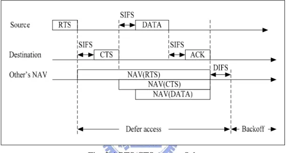
Obviously, a collision may occurs if two or more stations have detected the medium as idle for DIFS and both allowed to start their transmissions simultaneously. An ACK is used to notify the sender that the packet has been successfully received. After the expiration of the ACK timeout interval, the sender assumes that the packet was collided. So, it schedules a retransmission and starts the backoff procedure again. To resolve repeating collisions, after each unsuccessful transmission attempt, the CW is doubled until a maximum CW_max value is reached. After each successful transmission, the CW is reset to a minimum CW_min value. In radio systems based on medium sensing, the hidden station problem may occur. When a station is able to receive packets successfully from two senders but the two senders can not receive

signals from each other. To solve the problem, an optional RTS/CTS (Request to Send and Clear to Send) scheme is introduced. As shown in Fig. 2.4, the source sends a RTS packet to reserve the medium before each packet transmission and the receiver replies with a CTS packet if it is ready to receive. All other stations update their NAV whenever they sense an RTS, a CTS or a data frame and will not start their packet transmission until the NAV reached to zero.

Fig. 2.4 RTS/CTS Access Scheme

IEEE 802.11 uses three different InterFrame Spaces (IFS) to control the medium access.. A SIFS (Short InterFrame Space) period personates the highest priority to gain access to the medium and is used for ACKs, CTS frames and several following MPDUs of a fragment burst as well as for the response of a polled station in the PCF. In the CFP the point coordinator (PC) polls stations and must wait for a PIFS (PCF InterFrame Space) period which is longer than SIFS but smaller than DIFS. So, the period of different IFS described above should be specified as SIFS <PIFS <DIFS. The frame with higher transmission probability will wait shorter IFS period and get more chance to access the medium.

2.1.4 Point Coordination Function, PCF

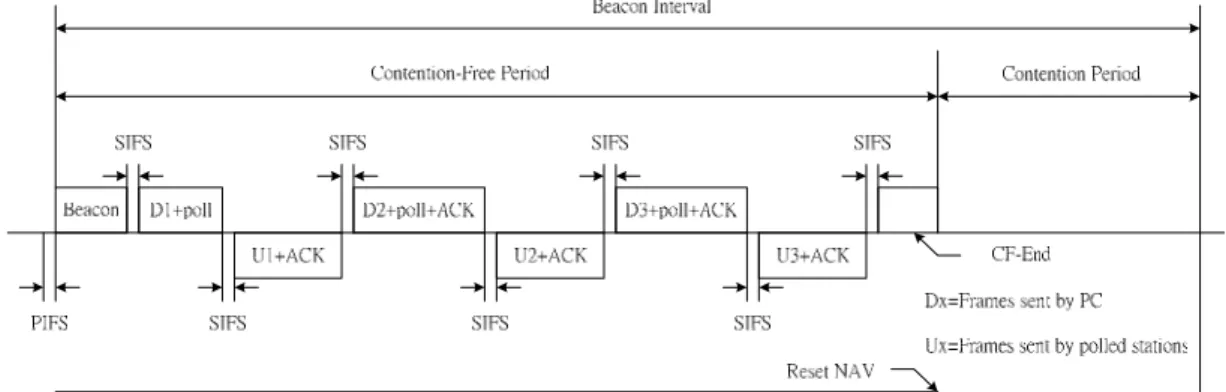
The PCF can only be used in an infrastructure-based network because it requires an access point (AP) as a point coordinator (PC). The PC manages the access to the medium in the CFP bye polling stations. In Fig. 2.5, the channel access time is divided into several beacon intervals and the beacon interval is composed of CFP and a CP. The PC polls all stations sequentially in the CFP. A polled station is allowed to answer with a data/ACK frame after waiting a SIFS time to the PC or to any other station in the network. In order to ensure that no DCF stations are able to interrupt the operation of the PCF, a PC waits for PIFS to start the PCF scheme. Then, all the other stations shall set their NAVs in the beginning of the CFP to the CFPMaxDuration value. If neither the PC nor the stations have frames to send, the CFP ends with a CFP-end frame sent by the PC and all receiving stations reset their NAVs and begins the CP. If the PCF is used for the transmission of time-bounded data, like video or voice, the PC should support a polling list. Every station listed there should be polled at least once per CFP. Due to its complexity, the PCF is mostly not implemented in current installed WLANs

2.2 IEEE 802.11e QoS Enhancement Standard

2.2.1 A brief of IEEE 802.11e standard

No priority mechanism is involved in DCF. All the packets are treated using the first come first serve philosophy. When the number of stations increases, the probability of collision becomes higher and results in performance degradation. Although PCF can support some time-bounded traffic, many problems have not been clearly solved, such as unknown transmission duration of polled stations and hard to predict the amount of frames stations want to send.

To solve these problems, the medium access schemes of IEEE 802.11 are enhanced to the upcoming future standard IEEE 802.11e. In this draft, a new method, Hybrid Coordination Function (HCF), is introduced to support QoS requirement. The architecture is described in Fig. 2.6. The HCF defines two medium access mechanisms: one is Enhanced Distributed Channel Access (EDCA) which is for the differential services requirement, and the other is HCF Controlled Channel Access (HCCA) which is used for the integrated services requirement. The EDCA manages the medium access in the CP while the HCF is responsible for the CFP and the CP.

Fig. 2.6 Diagram of IEEE 802.11e Architecture

traffic stream (TS) queues. When a packet arrives at the MAC layer, it is tagged with a traffic priority identifier (TID) according to its QoS requirement. The packets with TID values from 0 to 7 are mapped into four AC queues and those with TID values from 8 to 15 are mapped into eight TS queues which are specified in IEEE 802.1D, as in Table 2.1. The reason of separating TS queues from AC queues is to provide strict QoS at TS queues. Transmission opportunity (TXOP) is another feature of the HCF. TXOP is the time interval which is permitted for a certain station, getting the control of the medium, to transmit packets. During the TXOP, a station can transmit a series of packets separated by SIFS. If the frame exchange sequence has been completed, and there is still time remaining in the TXOP, the station can may extend the frame exchange sequence by transmitting another frame in the same access category. The station must ensure that the transmitted frame and any necessary acknowledgement can fit into the time remaining in the TXOP. The EDCA and HCCA mechanisms are respectively detailed in 2.2.2 and 2.2.3.

Table 2.1 Mapping of IEEE 802.1D User Priority to Access Category

2.2.2 Enhanced Distributed Channel Access, EDCA

station implements multiples ACs, as shown in Fig. 2.7. Each AC queue works as an independent DCF station and uses its own backoff parameters, that include minimum and maximum Contention Windows (CW_min, CW_max), Arbitration InterFrame Space (AIFS) and TXOP duration. These parameters are defining EDCA operation are store locally at the stations. These ones will be different for each access category (queue) and can be dynamically updated by the QoS access point (QAP) for each access category through the EDCA parameter sets. These are sent from the QAP as part of the beacon, and in probe and reassociation response frames. This adjustment allows the stations in the network to adjust to changing conditions, and gives the QAP the ability to manage overall QoS performance. Different IFS and CW sizes for different ACs are introduced to support service differentiation. Operation of each channel access function is similar to DCF. Data transmission begins when the medium is idle longer than the AIFS time, with AIFS ≥DIFS. The AIFS[AC] is determined by equation (2.2) and the default values of the Arbitration InterFrame Space Number (AIFSN) is defined in Table 2.2.

AIFS

[ ]

AC = AIFSN

[ ]

AC ⋅slot_time+SIFS (2.2)

As shown in Table 2.2, different CW sizes are allocated to different AC queues. Assigning a short CW size to a high priority AC ensures high-priority AC is able to transmit frames ahead of low-priority AC. If the backoff counter of two or more parallel ACs in a single station expires simultaneously, a scheduler inside the station treats the event as a virtual collision without recording a retransmission. Then, the TXOP is given to the high-priority AC and the other colliding ACs will enter a backoff process as if a collision on the medium occurred. AIFS is the extra time slots, appended at the beginning of each backoff contention window, which means the backoff random number is between AIFS and AIFS+CW, as shown in Fig. 2.8. Therefore, different ACs have different length of AIFS, thus reducing the probability of low-priority AC to be transmitted.

Table 2.2 the Default EDCA Parameter Set

Contention-based medium access is susceptible to severe performance degradation when overloaded. In overload conditions, the contention windows become large, and more and more time is spent in backoff delays rather than sending data. Admission control regulates the amount of data contending for the medium. EDCA admission control is mandatory at the AP, and optional at the station. The QAP may indicate that it requires stations to support admission control and explicitly request access rights by using the admission control mandatory (ACM) flags if they wish to use an access category. Admission control is negotiated by the use of a traffic specification (TSPEC). A station specifies its traffic flow requirements (data rate, delay bounds, packet size, and others) and requests the QAP to create a TSPEC by sending the ADDTS (add TSPEC) management action frame. The QAP calculates the existing load based on the current set of issued TSPECs. Based on the current conditions, the QAP may accept or deny the new TSPEC request. If the TSPEC is denied, the high priority access category inside the QoS station (QSTA) is not permitted to use the high priority access parameters, but it must use lower priority parameters instead. Admission control is not intended to be used for the best effort and background traffic classes, which classified as AC_BE and AC_BK respectively.

2.2.3 HCF Controlled Channel Access, HCCA

The HCF controlled channel access mechanism combines the advantages of PCF and DCF. HCF can start the controlled channel access mechanism in both CFP and CP intervals, as shown in Fig. 2.9. During the CP, a new contention-free period called controlled access phase (CAP) is introduced. CAPs are several intervals during which packets are transmitted using the HCCA mechanism. The station that operates as the central coordinator for all other stations within the same QoS supporting basic service

set (QBSS) is named the hybrid coordinator (HC). It is similar to PC which also resides within an IEEE 802.11e AP. HC can start a CAP by sending QoS CF-Poll frames to allocate polled-TXOP to different stations after the medium is idle at least PIFS period. During CFP, the starting time and maximum duration of each TXOP is specified and IEEE 802.11e backoff entities will not attempt to access the medium without being polled. Hence, only the HC can allocate TXOPs at this period. Then, the remaining time of the CP can be used by EDCA for stations contending for TXOPs, called EDCA-TXOPs. Polled-TXOP allocations may be delayed by the duration of an EDCA-TXOP. To solve this problem, the HC controls the maximum duration of EDCA-TXOPs by announcing the TXOPlimit

[ ]

AC for every AC via the beacon. So, HC is able to allocate polled-TXOPs at proper time during the beacon interval. When the certain delays of transmitted packets are required, HC may transmit a duration of TXOPlimit

[ ]

AC earlier than the optimal polled-TXOP allocation time to avoid any other packets deliver delay imposed by EDCA-TXOPs.

Fig. 2.9 A Typical HCF Beacon Interval [7]

In HCCA, QoS guarantee is based on the TSPEC negotiation between the QAP and QSTAs. In IEEE 802.11e draft, it provides the guidelines, for the design of a

simple scheduler and admission control unit, that meet the minimum performance requirements. In the scheduling recommended, each QSTA that is in the HCCA mode has first to send a QoS request packet to the QAP containing the mean data rate, the MAC Service Data Unit (MSDU) size and the maximum Service Interval (SI) required of the application which is using the TS. With these QoS information, the QAP determines the minimum of all the SIs required by different applications applying for HCCA. Then, it computes the highest submultiple of the beacon interval which is inferior to the minimum of all SIs. Therefore, the beacon interval is divided into several SIs and QSTAs in the QAP polling list are polled according to a round-robin algorithm during each SI. So, the QAP computes the individual TXOPs which will be allocated to the QSTAs after the SI is determined. For the calculation of the TXOP duration for an admitted stream, the scheduler uses the following parameters: Mean Data Rate (ρ) and Nominal MSDU Size (L ) from the negotiated

TSPEC, the SI calculated above, Physical Transmission Rate (R ), Maximum

allowable Size of MSDU and Overheads in time units (O). The calculation is described in equation (2.3) and (2.4).

_⎟⎟ ⎠ ⎞ ⎜⎜ ⎝ ⎛ + + × = O R M O R L N TXOP i i i i i max , (2.3) _⎥ ⎥ ⎤ ⎢ ⎢ ⎡ × = i i i L SI N ρ (2.4)

The TXOP allocation scheme ensures that the queue length of each TS having been polled in either constant or slowly decreasing in each round of polling by the QAP. An example is shown in Fig. 2.10. Stream from QSTA “i” is admitted. The beacon interval is 100ms and the maximum SI for the requested Stream is 60ms, so

the scheduler calculates a scheduled SI equal to 50ms, also determining the TXOP . _i

The same process is repeated continuously until the next maximum SI is larger the current SI. If a new stream is admitted or dropped, the scheduler needs to change the current SI and thus, the TXOP is recalculated with new SI again.

Fig. 2.10 An Example of Schedule for Streams form QSTA “i” to “k”

To improve the efficiency, the draft also introduced another two mechanisms, block acknowledgment and direct link protocol (DLP). Block acknowledgments allow a backoff entity to deliver a serious of MSDUs consecutively during one TXOP, each separated by a SIFS interval. The mechanism reduces the overhead of control exchange sequences by aggregating several acknowledgments into one frame. In the DLP mode, any station can directly communicate with any other station in a QBSS. The motivation of this protocol is that the intended recipient maybe in Power Save Mode, in which case it can be woken up by the QAP. So, the DLP prohibits the stations going into power-save for the duration of the direct stream as long as there is an active direct link set up between the two stations.

Chapter 3

Possible Improvement in Performance

3.1 Related Work

3.1.1 Possible Performance Improvement in MAC Layer

In the wireless local network field, many research works have been done to find out the theoretical performance and the probable improvement by introducing new medications and techniques. I discuss some of the existing analysis and researches in this chapter. My purpose is to find out a better way to improve the IEEE 802.11e draft protocol.

The new IEEE 802.11e standard is under developing on the basis of the IEEE 802.11 standard. The new standard must make full use of the physical channel, meet the special requirements of high priority packet flows and do resource reservation for some packet flows. IEEE has defined several traffic categories and traffic specifications. Each packet flow has its own requirement of maximum delay, minimum data rate and maximum delay jitter. In fact, if I have applied amount of bandwidth for the traffic including the overhead of the system, I can always achieve those performance requirements, like using HCCA for the time-bounded traffic. But, to be efficient or economical, the physical channel must be fully used for the payload as much as possible and the queue also must be particularly set up. Based on the IEEE 802.11 standard in MAC layer, I can find some possible improvements

described in the following.

In DCF or EDCA, each station transmits packets without knowing if there are any other stations also accessing the medium, and thus, collision happens and results in waste of medium time. The wireless station still does not have the ability to detect collision during the transmission procedure. So, it can only detect the failure when there is no reply from the receiver. If the packet is very long to send, the waste of bandwidth is high. For the view of improving the performance, the short packet may be better but may cause another problem, more overhead. The less collision occurs and the better performance exists. The solution for reducing the collision is to use a random number of slots to separate different transmissions from each other. The larger the backoff contention window, the less the probability of collision is. Obviously, if the contention window is too large, the wasted time due to idle slots might be larger than the wasted time due to collisions. Intuitively, the best solution is to queue up all the packets in all stations and transmit them sequentially. For this reason, there will be no waste of idle slots and no collision. Unfortunately, such an implementation needs a central controller which should know any information in the network, but the execution of the controller is not suitable for distributed systems, such as the DCF and EDCA mechanism. Another improvement on the IEEE 802.11e draft protocol is the traffic prediction, which is the spirit of the HCCA. In the HCCA mode, the AP must reserve enough bandwidth for some certain packets for each station in the BSS, but the AP is not very clearly and accurately aware of the amount of packets ready to transmit in the stations. Furthermore, some applications, like speech and videoconference signals have variable data rates and these make the prediction of the reservation harder, contrast to the application of the constant data rate. If the AP allocates the available bandwidth to the requested station too much, bandwidth waste occurs. On the contrary, if the AP allocates less bandwidth to the

requested station, performance degradation occurs. In order to achieve the better performance, one should trade off the two factors. In this theory, we do not chew over the HCCA. We concentrate on the improvement in EDCA.

3.1.2 Protocol Model and Performance Analysis of EDCA

In [9], Bianchi presented a simple and accurate Markov chain model to compute the throughput of a saturated IEEE 802.11 DCF network under ideal channel conditions. The model relies on two discrete time processes to model the progress of a given saturation through backoff. The analysis can help us a lot when we try to find some improvement methods for the IEEE 802.11e draft protocol. Two useful factors are introduced: the probability p that any transmission experiences a collision is constant and independent of the number of collisions already suffered; and the probability τ that a station will attempt transmission in a generic slot time. The key assumption in the model is that the conditional collision probability p is

given first, meaning that this is the probability of a collision seen by a packet being transmitted on the medium. According to the Markov chain, the transition probabilities of the system can be expressed as the equation (3.1).

}

(

)

( )

{

} (

)

(

)

( )

{

}

(

)

( )

{

}

(

)

{

⎪ ⎪ ⎩ ⎪ ⎪ ⎨ ⎧ = − ∈ = ∈ − ∈ = − ∈ − ∈ − = ∈ − ∈ = + m i W k W p m k m P m i W k W p i k i P m i W k W p i k P m i W k k i k i P m m i i i 1 , 0 0 , , , 1 1 , 0 0 , 1 , , 0 1 , 0 1 0 , , 0 , 0 2 , 0 1 1 , , 0 0 (3.1)

The index i is the number of collisions the packet suffered and k is the backoff value at the current time. m, maximum backoff stage, means the value such that CWmax 2 CWmin

m⋅

after the i -th collision. The first equation in (3.1) accounts for the spread of the

backoff value at the beginning of each slot time. The second equation explains the state varying after a successful transmission. The rest equations of (3.1) model the case after a failed transmission. Based on this model, ignoring the detailed calculations, we can express the probability τ as shown in equation (3.2).

₍

₎₍

(

₎

)

(

_m

)

p pW W p p ) 2 ( 1 1 2 1 2 1 2 − + + − − = τ (3.2)

W is the initial contention window, CWmin. In general, τ depends on the

conditional probability p . If there are n stations in the system, the relation between τ and p is in equation (3.3). To determine the maximum achievable saturation throughput, the probability τ can be approximated as equation (3.4) in the condition of saturation.

p=1−

(

1−τ

)

n−1 (3.3) 2 1 * c T n ≈ τ (3.4) * c

T is the duration of a collision measured in slot time. Equation (3.4) is of fundamental theoretical importance. It allows us to compute the optimal transmission probability τ in order to achieve the maximum throughput for each station. However, equation (3.2) and (3.3) show that maximum performance could be achieved for any considered network scenario, by suitably adjusting the system parameters m and W . Since the network size is not a directly controllable variable, the only way to achieve optimal performance seems to tune the values m

window size, the backoff window that maximizes the throughput is found as equation (3.5).

W_opt ≈n 2T_c* (3.5)

In [10] and [11], the authors extend Bianchi’s model to accommodate the QoS features provided by EDCA. They modify the Markov model described in [9] by introducing differential service parameters as show in Fig. 3.1. The major difference is the retry limit, m. Here, when the retry limit is reached, the retry number is reset to zero and recounted again until it reaches the limit m. The n-th traffic flow is associated with AIFS , _n CW_n,min, and CW_n,max. As the analysis in [9], they derive the traffic priority τ_n that a station transmits a packet in a randomly selected slot time. Assume there are total T priority traffic categories, and for each TC, the number of traffic flows is N , _t t =1,2,_LT . The total number of traffic flows is n, which is the summation of N . The traffic priority _t τ_n can be expressed as equation (3.6) and (3.7), the detailed calculation described in [10]. The relationship between the traffic priority and the conditional collision probability p is _n

expressed in equation (3.8), where λ_n is the backoff state transition rate.

_,0,0 1 1 1 n n m n n b p p − − = + τ (3.6)

₍

₎

(

)(

)

(

) (

)

(

1

)

1 0 , 0 , 1 2 1 1 ) 2 ( 1 1 2 1 2 + + _{− + − −} − − − = _m n n n m n n n n n n p p p p W p p b λ (3.7)

∏

(

)

≠ = − − = N n j j j n p , 1 1 1 τ (3.8) Under the assumption that the transmission queue of each traffic category is

always nonempty, this model can be used to calculate the throughput in the saturation condition by using the traffic priority τ_n and the probability p . From _n

equation (3.6) and (3.7), the influence on the throughput is determined by the parameters of each traffic category, m and W . The above analysis tells us that _n

maximum throughput can be tuned to achieve the same value, regardless of the number of transmitting station and the relation between the contention window and the maximum window size. So, the way to improve performance might be redirected to improve the use of the contention window mechanism, for example, adjusting

min CW with time. n λ λn λn λn λn n λ λn λn λn λn n λ λn λn λn λn n λ λn λn λn λn

Fig. 3.1 Markov Chain Model of EDCA

3.1.3 Adaptive EDCF, AEDCF

By adjusting the contention window to improve performance, we study a case in [12]. In [12], a method called Adaptive EDCF is proposed. The authors mention that the backoff strategy of IEEE 802.11e protocol has a defect, which is the contention window of the station is reset to the minimum value after each successful transmission. They proposed to reset the contention window values more slowly to

adaptive values, different to CW_min, taking into account their current sizes and the average collision rate while maintaining the priority-based discrimination. The value of the estimated collision rate f_currj is calculated using the number of collisions and the total number of packets sent during a fixed number of slot times, as expressed in equation (3.9). To minimize the bias against transient collisions, the authors use a smoothing factor α to adjust f_currj , described in equation (3.10). To ensure that the priority relationship between different priorities is still fulfilled when a class updates its contention window, each priority i should use different factor according to its

priority level, and the factor Multiplicator Factor (MF), as shown in equation (3.11), is introduced. Finally, the contention window is adjusted to equation (3.12).

_[

[

]

_]

attempt on transmissi of number E collisions of number E fcurrj = (3.9)

f_newj =

(

1−α

)

⋅ f_currj +α ⋅ f_newj−1 (3.10)

MF

[ ]

i =min

(

(

1+

( )

i⋅2

)

⋅ f_newj ,0.8

)

(3.11)

CWnew

[ ]

i =max

(

CWmin

[ ]

i,CWold ⋅MF

[ ]

i

)

(3.12)

Simulation results in [12] show that AEDCF increases the medium utilization ratio and reduces the collision rate with more than 50%. When achieving the delay differentiation, the overall gain of goodput is up to 25% higher than that of EDCA but the complexity of AEDCF remains similar to the EDCA scheme. In this paper, the author did not explain the mathematical basis of those formulas above, so we do not know if it is optimal. But there is a problem of fairness in this scheme. Since the spirit of AEDCF is to reset the contention window values to adaptive values

according to the network condition, the new contention window values of the stations that just successfully transmitted packets will be more competitive than those of the stations that failed to transmit packets. Usually, the contention window size will be doubled after unsuccessfully attempts and will be also larger than the new contention window value of the successfully transmitted station previously. So, this causes the unfairness of the stations of the same priority, especially in the case of the saturation condition.

3.2 Proposed Methods

In the EDCA mechanism, support of QoS can be easily achieved by reducing the probability of medium access for lower priority access categories. However, at high loadings of traffic, there are a large number of collisions even for high priority access categories so that the EDCA can not ensure achieving the QoS requirements since the EDCA is based on the CSMA/CA mechanism. Without a good admission control mechanism, the existing traffic can not meet the QoS requirements. In IEEE 802.11e, HCCA also provide guarantee QoS, but the mechanism is complex. In previous works, DCF is easier to achieve service differentiations than PCF, so it is the motivation to study the admission control mechanism based on the EDCA of IEEE 802.11e. In [13], [14], [15] and [16], the authors proposed some schemes to protect the existing real time traffic. We extend some of the authors’ ideas and propose new methods that provide procedures at the QAP and QSTAs for the contention-based admission control mechanism. All the procedures do not violate the guideline of the IEEE 802.11e draft and are able to greatly improve quality of services. In the proposed methods discussed below, the real-time traffic, such as

video and voice traffic, and the best-effort data traffic are handled separately.

3.2.1 Procedures for Real-Time Transmissions

On the receipt of an ADDTS request frame from a QSTA, the QAP shall make a determination as to whether to accept or deny the request according the algorithm implemented in it. The QAP maintains variables TXOPBudget

[ ]

i , SurplusFactor

[ ]

i

and ]TxTime[i for AC i , which i =1 for audio traffic, i=2 for video traffic, and i=3 for best-effort data traffic, respectively. TXOPBudget

[ ]

i is defined as the additional amount of time available for AC i during the next statistic period,

here using the Beacon interval, Target Beacon Transmission Time (TBTT), as the period. ]TxTime[i is used to record the time of the frame transmission and all overhead involved such as SIFS and ACK frame corresponding to the AC of that frame. SurplusFactor

[ ]

i is used for calculating the unpredictable time, such as collisions or retransmissions. So, the TXOPBudget

[ ]

i is determined by equation (3.13), where ATL[i] is for the maximum amount of time that may be used for transmissions of AC i per beacon interval.

TXOPBudget[i]=max

(

ATL[i]−TxTime[i]×SurplusFactor[i],0

)

(3.13)

Each QSTA has to maintain the following local variables for AC i : ]TxUsed[i , ]

[i

TxSuccess , ]TxLimit[i , ]TxRemainder[i , and TxMemory[i]. ]TxUsed[i counts the amount of time occupied by transmissions. TxSuccess[i] counts for the successful transmission time. TxRemainder[i] is defined as equation (3.14).

] [i

TxLimit limits the maximum time that a QSTA could be used to transmit. A

transmit. ]TxMemory[i memorizes the amount of time that a QSTA transmit frames of priority i . All these variables update at each TBTT, and will be exploited in next

TBTT.

TxRemainder[i]=TxLimit[i]−TxUsed[i] (3.14)

So, if the TXOPBudget[i] becomes zero, new QSTAs can not start transmission with AC i and the other QSTAs’ TxMemory[i] remains unchanged. In other words, when the transmission budget for an AC i is depleted, new QSTA

can not transmit frames of priority i , while the exiting traffic of priority i can not

increase the admitted time. At this moment, new QSTA which want to transmit AC

i traffic should change the parameters to lower priority class according to the IEEE

802.11e standard. If the TXOPBudget[i] is larger than zero, meaning that there is still enough resource, new traffic of priority i is allowed to transmit and its

] [i

TxMemory is a random time between 0 and

] [ ]

[i SurplusFactor i

TXOPBudget . The other QSTAs’ TxMemory[i] is a weighted average of the old TxMemory[i] and the sum of TxSuccess[i] and

] [i

TXOPBudget , as equation (3.15), where f is the damping factor to effect the

weighted value.

(

1

) (

[] [ ] []

)

] [ ] [ i TXOPBudget i tor SurplusFac i TxSuccess f i TxMemory f i TxMemory + × × − + × = (3.15)

As time goes, TXOPBudget[i] fluctuates around 0 and TxMemory[i] converges to the value TxSuccess[i]×SurplusFactor[i], which is the lower limit for each QSTA. The meaning of equation (3.15) is that an existing traffic of a QSTA can continuously consume the same amount of time in subsequent TBTT. The procedure is used for the video and voice traffic, so the existing real-time traffic is protected

from the new and other existing real-time traffic and then the QoS requirements could also be achieved under high loads. An example shown in Fig. 3.2 is to explain the mechanism. The ATL[1] and ATL

[ ]

2 represent the maximum amount of time used for transmissions of AC 1 and 2 respectively.

TBTT ATL[1] ATL[2] TxTime[1]*SurplusFactor[1] TXOPBudget[1] TBTT ATL[1] ATL[2] TxTime[1]*SurplusFactor[1] TXOPBudget[1]

Fig. 3.2 The Calculation of Transmission Budget

At the certain TBTT, QAP calculated TXOPBudget[1] from equation (3.13) and broadcasts the value to QSTAs via beacon frames, so does TXOPBudget[2]. When QSTAs receive the value of TXOPBudget[1] and TXOPBudget[1] is larger than zero as in Fig. 3.3, new TxMemory[1] is calculated form equation (3.15) which utilizes the TXOPBudget[1]. If another new QSTA, S4, wants to transmit traffic of AC 1, it makes use of TXOPBudget[1] by random determining the value between 0 and TXOPBudget[1] SurplusFactor[1] . All these variables,

] 1 [

r

TxRemainde , ]TxMemory[1 , and TxLimit[1] of QSTA1, QSTA2, etc., should be calculated before transmitting. Obviously, if the TXOPBudget[1] becomes zero, there is not enough budget for admitting new traffic of AC 1 . So, the

4 _ ] 1 [ S

TxMemory is zero, meaning that the new QSTA, S4, can not transmit this traffic of AC 1 and the other QSTAs’ TxMemory[1] remain unchanged in next TBTT.

TxLimit[1]_S1 TxMemory[1]_S1 TxRemainder[1]_S1 S2 S3 TXOPBudget[1] S2 S3 S4 TXOPBudget[1] TxLimit[1]_S1 TxMemory[1]_S1 TxLimit[1]_S1 TxMemory[1]_S1 TxRemainder[1]_S1 S2 S3 TXOPBudget[1] S2 S3 S4 TXOPBudget[1] TxLimit[1]_S1 TxMemory[1]_S1

Fig. 3.3 An Example of Utilizing the Transmission Budget

3.2.2 Procedures for Best-Effort Data Transmissions

Since the best-effort data transmissions, which is classified AC 0, do not need guaranteed QoS, the QAP dynamically control the parameters for QSTAs based on the traffic condition. These parameters are CW_min[0], ]CW_max[0 , and AIFS[0] which will effect the throughput of data transmissions. The reasons of dynamically controlling the parameters are described as follows. Too many data transmissions may degrade the performance of the existing video or voice traffic. In this case, data throughput should be decreased. On the other hand, if the channel condition becomes better and the performance of the video or voice traffic does not degrade a lot, we shall increase the data throughput as possible. However, the decision of increasing or decreasing the data throughput should be made according additional conditions, like if the successful transmission time of real-time traffic is increasing or not, in order not to cause a great damage to time-bounded traffic due to an aggressive approach to these parameters.

The variables used for QAP to understand the channel condition are

STT

QoS _ , Data _STT, FTT , and Idle _Time, as shown in Fig. 3.4, where

STT

QoS _ is the sum of the successful transmission time of all real-time traffic,

STT

total failure transmission time of all kinds of traffic, and Idle _Time is the time measured by QAP when the medium is idle.

TBTT

QoS_STT Data_STT FTT Idle_time

TBTT

QoS_STT Data_STT FTT Idle_time

Fig. 3.4 The Diagram of STT, STT, and Idle

Based on judgments of an increased/decreased value of QoS _STT, FTT or Time

Idle _ , we propose an algorithm of controlling the data parameters to

maximize the data throughput under the condition of protecting the existing real-time traffic. The control mechanism is shown in Fig. 3.5. α and β denote a predefined successful ratio and a predefined failure ratio, respectively. First, we check if the throughput of the existing real-time traffic increases or decreases. Second, at high loads, the channel is idle usually due to the same backoff slots between QSTAs after each unsuccessful attempt. At this case, if Idle _Time is larger than Threshold, we prefer to shorten the contention window size; otherwise, we enlarge the contention window size. However, the increase of Idle _Time

might be the cause of the existing traffic leaving. FTT is the third criterion of

judgments on the case of suddenly leaving. In Fig. 3.5, all eight conditions are considered. θ

( )

t =1 denotes an increase of parameters for data at time t and

means the decreasing of the data traffic load. θ

( )

t =−1 denotes a decrease of parameters for data at time t and means the increasing of the data traffic load.

( )

t =0

θ represents remaining unchanged. In our simulation, we adopt the linear increasing/decreasing of these parameters, i.e. CW_min[0]= CW_min[0]±∆₁ ,

2 max

max[0]= CW [0]±∆

CW , and AIFS[0]= AIFS[0]±∆₃.

Bianchi’s work to estimate the mean idle time. Let τ_i be the stationary probability that a flow i transmits a packet in a randomly selected slot time, as equation (3.16).

In the context of this case, a flow i is defined as a set of packets belonging to the

data traffic of a QSTA and uses the same parameters. p denotes the collision _i

probability of flow i . Wis the size of CW_min used for flow i . m is the value such that CW mW 2 max = .

₍

₎₍

(

₎

)

(

_m

)

i i i i i p W p W p p ) 2 ( 1 1 2 1 2 1 2 − + + − − = τ (3.16) ( )t =0 θ θ( )t =−1 θ( )t =1 α ( )t =0 θ θ( )t =−1 ( )t =0 θ ( )t =0 θ ( )t =1 θ β β β β

Then, the probability of all the n QSTAs being idle in a randomly chosen time slot is q= 1

(

−τ_i

)

n. The probability that there is at least one transmission in a slot is 1−q. Hence, the mean number of idle slots is shown in equation (3.17). The problem is, we still do not know the τ_i. However, in [4], the approximate solution of τ_i is as equation (3.18).

[ ]

(

)

slot time q q kq q time slot idle E k k _ 1 1 _ 1 × − = × − × =

∑

∞ = (3.17) T n i 2 2 ≈ τ (3.18)

Now τ_i depends only on n and T , where T is the duration of a collision

measured in slot time units, in [4] discussed more. Let us consider the equation

(

)

n i

q= 1−τ . We get the approximate value q=

(

1−2 n 2T

)

n. Since the part

T

2 2 −

is a constant, this formula can be simplified when n→∞, as equation (3.19).

q≈e−2 2T, T =PHY_hdr +Payload +DIFS (3.19)

The approximate value of q is a constant. Suppose we are using IEEE 802.11a standard, then: DIFS =34µs , PHY_hdr =24µs ,

s Mbps bits Payload 222.2µ 54 8 * 1500 ₌

= , and slot_time=9µs . Therefore, we get

1333 . 31 ≈ T time slots, ≈ −0.25345 =0.7761 e

q , and E[idle]=0.031ms . Simply speaking, the QSTA only has to wait for the average idle time before a transmission. Our Threshold is changed with time and defined as equation (3.20), where

TBTT t

the lower bound of predicted idle time. If the Idle _Time measured in one TBTT is larger than the Threshold, the reaction is to shorten the contention window size of data traffic to increase the throughput, or enlarge the contention window size in the other case. So, at high loads, we use Threshold to determine whether we should increase the data traffic or not.

Threshold =TotalPacket_TBTT×E

[ ]

idle (3.20)

Since the QAP determines the parameters of data traffic in one TBTT and will broadcast them via Beacon frames, QSTAs only reassign their own CWmin[0],

] 0 [

max

Chapter 4

Performance Evaluation

4.1 Simulation Scenario

All scenarios have been implemented in the network simulator (NS2, 2.1b7) [17]. In these simulations, there are no hidden stations and the channel is assumed to be error free. The simulation topology is shown in Fig. 4.1. Table 4.1 shows the IEEE 802.11a PHY/MAC parameters used in these simulations and Table 4.2 shows the network parameters selected for the three ACs.

Fig. 4.1 Simulation Topology

SIFS 16µs DIFS 34µs

PHY Rate 54Mbps Minimum Bandwidth 6Mbps

Slot Time 9µs PHY Header 24bytes

Preamble Length 20µs PCLPHeader Length 4µs

CCATime 4µs RxTxTurnaroundTime 2µs

aCWmin 15 aCWmax 1023

IP Header Size 20bytes UDP Header Size 8bytes

Parameters Audio Video Best-effort Data

Priority High Medium Low

CWmin 3 7 15 CWmax 7 15 1023 AIFSN 2 2 7 Packet Size(bytes) 160 1080 1500 Packet Interval(ms) 20 2.16 12 Sending Rate(Kbps) 64 4000 1000

Table 4.2 MAC Parameters for the Three Traffic Categories

4.2 Priority Test

Fig. 4.2 is an example of throughput of different streams to test the priority. In this case, one QAP and only one QSTA are in the BSS and the payload of each stream is 1500 bytes for comparing the priority only without any other factor, like fragmentation. The audio stream tries to transmit 64Kbps, the video stream tries to transmit 10Mbps, and each of the other two data streams tries to transmit 15Mbps. Audio, video and Data_1 start at the same time. Before 8 seconds, there is enough network capacity, the audio and video achieves their own transmission rates, 64Kbps and 10Mbps respectively, so does Data_1, 15Mbps. After 8 seconds, Data_2 starts to send packets. However, the network capacity is not sufficient, so the two data streams share the remaining sources and the throughput of audio and video still remains their own transmission rates. The example shows that when the network capacity is enough, the lower priority traffic makes use of the extra resources. When the capacity is insufficient, the throughput of higher priority traffic is still maintained while the lower priority traffic shares the remaining sources. The bandwidth shown in Fig. 4.2 is the average bandwidth. From our test, the maximum throughput for 1500 bytes payload is 24.76Mbps

which is close to 25Mbps calculated in [18] and indirectly proves the correctness of our implementation model since we have made a lot of changes in NS-2 module.

Fig. 4.2 Priority Test for Different Streams

The mean latency is shown in Fig. 4.3. After 8 seconds, the mean latency of audio or video traffic is both lower than 1ms. But, the mean latency of data_1 or data_2 is larger than 100ms which proves the lower priority is suppressed to transmit when the network capacity is not sufficient.

4.3 Simulation Results for DCF and EDCA

The simulation results of bandwidth with DCF and EDCA mechanisms are shown in Fig. 4.4 and Fig. 4.5 respectively. The mean delay is shown in Fig. 4.6 and Fig. 4.7. There are total 15 traffic streams in this scenario, five for each AC, and the parameters are set as Table 4.2. By comparing Fig. 4.4 and Fig. 4.5, which plot the throughput of each traffic stream, we observe that the throughput of video and data are significantly different for DCF and EDCA. The video traffic is well served with EDCA while there are many packets dropped with DCF. The mean delay of video and voice traffic for EDCA is around 1ms, but for DCF, the mean delay of video is larger than 50ms. The mean delay of data traffic for EDCA is far larger than that of real-time traffic, which tells us again that the transmission lower priority is suppressed in order to increase the transmission probability of the higher priority. So, EDCA can achieve QoS requirements for real-time traffic if there is enough network capacity.

However, if we add a new video stream to increase the channel loading, at high loads, EDCA can not perform well as in low loads, as shown in Fig. 4.8. In Fig. 4.9, the latency of video is larger than 100ms, so the transmission of video is almost unpractical at this case. Therefore, we proposed our methods to solve the problem described in Chapter 3.2 and the method is more easily implemented than HCCA, which has the same purpose to improve the performance of the real-time traffic in wireless network.

Fig. 4.4 The Throughput for DCF

Fig. 4.6 The Mean Latency for DCF

Fig. 4.8 The Throughput for EDCA at High Loads

4.4 Simulation Results for the Proposed Method

In this section, we study the performance of our proposed method. Table 4.2 shows the parameters of traffic streams. The SurplusFactor of all real-time traffic is

1 .

1 , ALT[1]=0.7×100ms=70ms , ALT[2]=0.2×100ms=20ms , the beacon interval is 100ms, and the damping factor f is 0.9. At the beginning, there are six audio streams, five video streams and two best-effort data streams in the system. At the time 10s, another two video streams arrive. Fig. 4.10 and Fig 4.12 show that if the procedure of protecting the existing real-time traffic described in Chapter 3.2.1 is not implemented in QAP, the performance of video stream is terrible. But if the protected procedure is implemented, QoS of the existing performance is guaranteed as in Fig. 4.11 and Fig. 4.13. The reason why the new arriving video streams still be transmitted at 0.1Mbps is that TXOPBudget[2] still remains resources at high loads so that the new streams can make use of it to provide more services.

Fig. 4.11 The Mean Latency of EDCA without Protecting Real-Time Traffic

Fig. 4.13 The Mean Latency of EDCA with Protecting Real-Time Traffic

Next, we extend the scenario to test the second proposed method described in Chapter 3.2.2. α and β are set equal to 0.8. ∆1 is set to 10, ∆2 is set to15,

3

∆ is set to 0, E[idle]=0.031ms and Threshold is calculated from equation (3.20) dynamically changing with beacon interval. If new three data traffic streams arrival at the time 25s, the performance of video traffic is degraded again, as show in Fig. 4.14 and Fig. 4.15. After the implementation of the second proposed method, the real time traffic is protected again because the procedure lowers the throughput of data traffic after the time 25s as in Fig. 4.16 and Fig. 4.17.

Through the simulation, obviously our proposed methods are workable. Therefore, with the control of real time traffic and best-effort data traffic, the network system can easily achieve the requirements of QoS.

Fig. 4.14 The Throughput of EDCA without Data Control

Fig. 4.16 The Throughput of EDCA with Data Control

Chapter 5

Conclusion

In thesis, we have given an overview of the IEEE 802.11e and evaluated the performance, in transmitting QoS applications. The block acknowledgment and direct link protocol are not implemented in our simulation model. How to apply these two mechanisms to enhance the QoS and to automatically change ATL[i] with network capacity is the future work.

Through our simulations, we find that although EDCA could provide a service differentiation among different access categories, it is still deficient in QoS guarantee at heavily loaded traffic network conditions under huge amount of best-effort traffic. In such case, we proposed the schemes of protecting the existing real time traffic and suitably controlling the best-effort data to avoid damaging the performance of the time-bounded traffic. For voice and video streams, QSTAs listen the budget from QAP to determine on accepting or rejecting the new streams. For best-effort data transmission, QAP dynamically control the data parameter based on the traffic condition. Under the implementation of these schemes on QAP and QSTAs, QoS requirements from heavy load traffic in EDCA mode could be better satisfied.

Bibliography

[1] IEEE Std. 802.11, "Wireless LAN Medium Access Control (MAC) and Physical

Layer (PHY) Specifications,” 1999.

[2] IEEE Std. 802.11e/D5.1, "Medium Access Control (MAC) Enhancements for

Quality of Service (QoS),” October 2003.

[3] D. Chen, D. Gu and J. Zhang, "Supporting Real-Time Traffic with QoS in IEEE

802.11e Based Home Networks," Consumer Communications and Networking

Conference (CCNC), pp. 205-209, January 2004

[4] S. Choi, JD Prado, S. Shankar and S. Mangold, "IEEE 802.11e contention-based

channel access (EDCF) performance evaluation," in Proc. IEEE ICC'03, vol. 2,

pp. 1151-1156, May 2003.

[5] T. S. Ho and K. C. Chen, "Performance evaluation and enhancement of the

CSMA/CA MAC protocol for 802.11 wireless LAN’s," in Proc. IEEE PIMRC,

Taipei, Taiwan, pp. 392-396, October 1996.

[6] L. Yang, "P-HCCA: A New Scheme for Real-time Traffic with QoS in IEEE

802.11e Based Networks," APAN Network Research Workshop 2004.

[7] Q. Ni, L. Romdhani, and T. Turletti, "A Survey of QoS Enhancements for IEEE

802.11 Wireless LAN," Journal of Wireless Communications and Mobile

Computing, vol. 4, no. 5, pp. 547-566, August 2004. [8] B. Walke, Mobile Radio Networks, 2nd ed., Wiley, 2001.

[9] G. Bianchi, "Performance analysis of the IEEE 802.11 distributed coordination function," IEEE Journal on Selected Areas in Communications, pp. 535-547,

March 2000.

[10] H. Zhu and I. Chlamtac, "An Analytical Model for IEEE 802.11e EDCF

Differential Services," IEEE ICCCN3, Dallas, October 2003.

[11] J. Gosteau, M. Kamoun, S. Simoens, P. Pellati, "Analytical developments on QoS

[12] L. Romdhani, Qiang Ni, and T. Turletti, "Adaptive EDCF: enhanced service

differentiation for IEEE 802.11 wireless ad-hoc networks," IEEE Wireless

Communications and Networking, vol. 2, pp. 1373 – 1378, March 2003.

[13] Y. Xiao, H. Li, and S. Choi, "Protection and Guarantee for Voice and Video Traffic

in IEEE 802.11e Wireless LANs," Proc. of IEEE INFOCOM 2004.

[14] Y. Xiao and H. Li, "Voice and Video Transmissions with Global Data Parameter

Control for the IEEE 802.11e Enhance Distributed Channel Access," IEEE

Transactions on Parallel and Distributed Systems, vol. 15, no. 11, pp. 1041-1053, November 2004.

[15] Y. Xiao and H. Li, "Evaluation of distributed admission control for the IEEE

802.11e EDCA," IEEE Communications Magazine, vol. 42, pp. S20 - S24,

September 2004.

[16] D. Pong and T. Moors, "Call Admission Control for IEEE 802.11 Contention

Access Mechanism," In Procceedings of IEEE Globecom, 2003.

[17] Berkeley Network Simulator ns-2. http://www.isi.edu/nsnam/ns.

[18] T. Cooklev and V. Shah, "Throughput of 802.11e, assuming 802.11a, 802.11b, or

802.11g physical layers," IEEE 802.11 interim meeting, Sept. 2004, document