檢定兩個自迴歸移動平均模型或兩個隨機係數自迴歸模型的相等性

國立交通大學

統計學研究所

碩士論文

檢定兩個

自迴歸移動平均模

型或兩個隨機係數自迴歸

模型

的相等性

Testing equality of two ARMA models or two random

coefficient autoregressive models

研 究 生: 鍾興潔

指導教授: 王秀瑛 教授

檢定兩個自迴歸移動平均模型或兩個隨機

係數自迴歸模型的相等性

研究生:鍾興潔 指導教授:王秀瑛 博士

國立交通大學理學院

統計學研究所

摘要

時間序列分析是一套動態數據處理的統計方法。基於隨機過程及數理統計理 論，分析變數的產生與變數間之動態關係，進而能檢定經濟理論或對變數進行預 測，以用於解決實際問題，其中，又以 Box-Jenkins 的自迴歸移動平均模型之分 析方法最廣為被大家所使用。此外，理論的發展與推廣，時間序列模型至今已發 展到相當複雜的程度，隨機係數自迴歸模型（Random Coefficient Autoregressive model；RCA）便是一個值得深入研究的主題，在這篇論文裡，我們提出檢定兩 個自迴歸移動平均模型相等性的方法以及檢定兩個隨機係數自迴歸模型相等性 的方法，並且在我們的模擬結果中顯示，我們的方法確實能使該檢定的型一錯誤 達到我們設立的顯著水準。我們應用這個分析方法在實際的公司營收資料上，在 我們所分析的三間公司中，顯示出有兩間公司的營收在我們所配適的模型上有顯 著的差異。 關鍵詞：時間序列、自迴歸移動平均模型、隨機係數自迴歸模型

Testing equality of two ARMA models or two

random coefficient autoregressive models

Student: Singjie Jong

Advisor: Hsiuying Wang

Institute of Statistics National Chiao

Tung University Hsinchu, Taiwan

Abstract

This thesis addresses the issues of testing equality of two time series models. Testing procedures for testing the equality of two ARMA models or two random coefficient autoregressive (RCA) models are proposed. For testing the equality of two ARMA models, we based on the maximum likelihood estimators to establish a testing procedure. For testing equality of two RCA models, an empirical likelihood method is developed. The proposed methods have been demonstrated to have good properties and are shown to have good performance through simulation studies. Also, the testing procedure for testing the equality of two ARMA models is illustrated through an analysis of three companies’ monthly sales.

誌謝 首先，很感謝我的的指導老師王秀瑛 教授。在跟老師相處的一年多時間， 老師總能給我很多好的方向及構想，並且不斷的給予我鼓勵，除了讓我學習到統 計上的專業知識及應用，也培養了積極樂觀的人生態度，我相信在這樣子的薰陶 之下，往後出社會所面臨的挑戰，都能夠迎刃而解。再來要感謝口試委員：黃榮 臣 教授、江永進 教授、以及洪慧念 教授 在口試時對於我的論文提出更佳之建 議及修改方向，使我此篇研究結果能更加完整，我也要感謝在這兩年，所修過課 或旁聽過課的任教老師: 刁錦寰 教授、徐南蓉 教授、盧鴻興 教授、陳鄰安 教 授、黃冠華 教授及陳志榮 教授，老師們的教導對於我的論文都有許多直接或間 接的幫助。 在碩士班兩年的期間，我要感謝研究所的所有同學，感謝小胖、魯夫、蟲蟲、 沒空、大鳥、小蜜蜂、鐿瀞、宜靜、亭育、貓貓、翁哥、阿鴻、偉振、老大、心 機、俞伶、家榕、mo …等族繁不及，當我心情鬱悶時，同學們總能適時的提供 各種抒壓的管道，使我擁有再戰的動力，在課餘時，能和研究室的同學一起聊天 打球跑步游泳玩桌遊，是何等快樂的事情，讓我在碩士生涯的兩年期間過的相當 愉快，另外，我也要感謝在桃園的好朋友們：嘟嘟、逸仙、阿肥、小香、小悟， 感謝這兩年來在精神上與生活上的許多幫助。 最後，我要感謝最支持我的父母及哥哥，親情力量，何等偉大，這兩年的 研究生活，總有許多不如意的時候，家人是給我無比的鼓勵及安慰，讓我能全心 全意地專注在研究上。在這一路上，感謝大家的幫助與指引，希望我的努力能讓 你們感到欣慰與驕傲。 鍾興潔 謹誌于 國立交通大學統計學研究所 中華民國一百零一年六月

Contents

1 Introduction 1

2 A Test of Equality of ARMA Models 3

2.1 Introduction . . . 3

2.2 Basic Results . . . 5

2.3 Testing Methods . . . 8

2.4 A simulation study . . . 10

3 A Test of Equality of RCA Models 12 3.1 Introduction . . . 12 3.2 Basic Results . . . 13 3.3 Testing Methods . . . 15 3.4 A simulation study . . . 16 4 Application 18 5 Conclusions 29

List of Figures

4.1 Monthly Sales of FamilyMart, President Chain stores and Poya . . . . 23 4.2 the ACF of the first differneces of the natural logarithms. . . 24 4.3 the ACF of both series took log and two difference (lag 1 and lag 12) . 25 4.4 the PACF of both series took log and two difference (lag 1 and lag 12) 26 4.5 the ACF and PACF of residuals of the ARMA(3, 0)(2, 0)12 model of Z1t 27

4.6 the ACF and PACF of residuals of the ARMA(3, 0)(2, 0)12 model of Z2t. 27

4.7 the ACF and PACF of residuals of the ARMA(3, 0)(2, 0)12model fitting

List of Tables

2.1 Testing the equality of two AR(1) models at level 0.05 (difference sample

size setting) . . . 10

2.2 Testing the equality of two AR(1) models at level 0.05 (difference β setting) 11 2.3 The bonferroni method for testing the equality of two AR(2) models at level 0.05 . . . 11

2.4 The Chisque method for testing the equality of two AR(2) models at level 0.05 . . . 11

3.1 The EL method for testing the equality of two RCA(1) models at level 0.05 . . . 17

4.1 The 145 records for the monthly sales of FamilyMart . . . 21

4.2 The 145 records for the monthly sales of President Chain Store . . . 21

4.3 The 145 records for the monthly sales of Poya . . . 22

1

Introduction

Time series analysis is an area of considerable activity. In the past, economists was using time series for microeconometrics, but they did not carefully explore their statistical properties. Box and Jenkins (1979) rebuild our vision of time series analysis, and then a bunch of books and articles on the subject have been published. The theories and methods have been well estabished and its influence continue to rise. For example, Shumway and Stoffer (2000) presented a balanced and comprehensive treatment of both time and frequency domain methods with accompanying theory and Brockwell and Davis (2009) provided specific techniques for handling data and at the same time to provide an understanding of the mathematical basis for the techniques. Now, time series analysis is used for many applications such as economic forecasting, sales forecasting, stock market analysis, process and quality control.

The time series data in practical problems may consist of observarions from a vector of numbers. For example, in sales forecasting, the variables include sale volume, prices and sales force, and then we can use a multivariate form of the Box-Jenkins model to analyze how is the influence of prices and sales force on sale volume. However, in multivariable time series analysis, we concentrate on input-output relationship between dependent variables and independent variables, and we rarely see the discussions about the comparion of two time series. In the above example, if there are two companys in the study, equality of two company’s sales force effect on the prices may be our interests.

On the other hand, nonlinear time series models have attracted much interest during there years. Although most of the time series models discussed are linear models, it has often been found that linear models usually lead to some unexplained aspects. Many developments in nonlinear models techniques provide some alternatives to model time series, and one of examples is the random coefficient model. For this reason, we also pay attention to the comparion of two random coefficient autoregressive (RCA) time series model.

In this article, we are interented in compare two ARMA models or RCA mod-els. Two proposed methods are introduced step by step in the following chapters for ARMA models and RCA models. In additional, we conduct simulation studies for eval-uating the performance of both methods. Finally we performe our methods to real data analysis and concluding remarks are given.

2

A Test of Equality of ARMA Models

2.1

Introduction

There are many methods for modeling time series data, and the most widely recognized approach is the Box-Jenkins ARMA models. Classical Box-jenkins models describe stationary time series. A time series {xt; t ∈ Z}, with Z = 0, ±1, ±2, ... is

stationary if

(1)E|xt|2 < ∞ for all t ∈Z

(2)E(xt) is constant for all t ∈Z

and

(3)rx(r, s) = rx(r + t, s + t) for all r, s, t ∈Z,

where rx(r, s) = cov(xr, xs) = E(xr− E(xr), xs− E(xs)) for all r, s ∈Z.

A time series {xt} with zero mean is an ARMA(p, q) model if it is stationary and

xt= φ1xt−1+ .... + φpxt−p+ ωt− θ1ωt−1− .... − θqωt−q (2.1)

with φp 6= 0, θq 6= 0. Unless stated otherwise, the noise ωt is iid ∼ N(0, δω2), where

δ2

ω > 0. Also, the parameters p and q are called the autoregressive and the moving

average orders, respectively. To express the ARMA models in an easy formula, it will be useful to write them using the AR operator and the MA operator. That is, we

rewrite the formula (2.1) as

φ(B)xt = θ(B)ωt (2.2)

where φ(B) = 1 − φ1B − φ2B2− ... − φpBp, and θ(B) = 1 − θ1B − θ2B2− ... − θqBq. On

the other hand, since the relationships between past and future often occur at seasonal lags, it is appropriate to consider seasonal ARIMA models. The seasonal ARMA model of orders P and Q with the seasonal lags s, denoted by ARMA(P, Q)s, is of the form

ΦP(Bs)xt = ΘQ(Bs)ωt,

where φ(Bs_{) = 1−φ}

1Bs−φ2B2s−...−φPBP s, and θ(B) = 1−θ1B −θ2B2s−...−θQBQs.

We only consider causal and invertible ARMA models in this article. An ARMA(p,q) process defined by equation (2.2) is said to be causal if there exists a sequence of con-stants ψj such that

∞ X j=1 |ψj| < ∞ and xt = ∞ X t=1 ψjωt−j, t = 0, ±1, ±2, ...

and said to be invertible if there exists a sequence of constants πj such that ∞ X j=1 |πj| < ∞ and ωt= ∞ X t=1 πjxt−j, t = 0, ±1, ±2, ...

Since seasonal models are special forms of the ARMA models, the description of the parameter properties is not repeated here.

We consider two time series xt and yt which both are ARMA(p,q) process with

the forms

xt = φx,1xt−1+ .... + φx,pxt−p+ θx,1ωx,t−1+ .... + θx,qωx,t−q (2.3)

yt = φy,1yt−1+ .... + φy,pyt−p+ θy,1ωy,t−1+ .... + θy,qωy,t−q (2.4)

Denote β

x = (φx,1, ..., φx,p, θx,1..., θx,q) ′

and β

y = (φy,1, ..., φy,p, θy,1..., θy,q) ′

, respec-tively. We are interested in testing the equality of two time series models, this is, β_x =β_y.

In this chapter, we introduce the Box-Jenkins approach for an ARMA model. The porperties and calculations of MLE are also discussed. In particular, the confidence interval for parameters of ARMA models based on MLE can be obtained in an easy way after estimating parameters. Next, we proposes two methods for constructing approximate CI based on MLE, and simulation studies which demonstrates their false positive rate are shown.

2.2

Basic Results

Maximum Likelihood Estimation (MLE) is one of the most popular parameter estimation in time series model, since it possesses a number of good asymptotic prop-erties. However, in the general ARMA models, it is hard to express the likelihood as a function of parameters directly. For this reason, Shumway and Stoffer (2006) suggested to substitute a function of the one-step prediction errors for the explicit way to write the likelihood function. If xt is causal ARMA(p,q) process with zero mean, the likelihood

function of xt can be written as L(β_x, δ2_ω) = n Y t=1 f (xt | xt−1, ..., x1),

The distribution of xt given xt−1, ..., x1 is a Gaussian distribution with mean xt−1t =

E(xt | xt−1, ..., x1) and variance Ptt−1 = V ar(xt | xt−1, ..., x1). In addition, for ARMA

models, we may write P_tt−1 =δ2

ωrt−1t where rtt−1 does not depend on δω2. In here, xt−1t

and variance P_tt−1 are also called the one-step predictor and the mean square prediction error, respectively. They can be solved iteratively by Durbin-Levinson Algorithm (see Durbin, 1960 ). Now, we rewrite the likelihood function of xt as

L(β_x, δ2ω) = (2πδω2) −n/2 [r01(β_x)r21(β_x) . . . rn−1n (β_x)] −1/2 exp[s(βx) 2δ2 ω ], (2.5) where s(β_x) = n X t=1 [(xt− x t−1 t (β_x))2 rt−1_t (β_x) ]

Since xt−1t and Ptt−1 are explicitly functions of β_x and δω2, we can obtain maximum

likelihood estimation by maximizing (2.5).

Under appropriate conditions (see Shumway and Stoffer, 2006 p.133 and Brockwell and Davis, 2006 p.258), the maximum likelihood estimation bβ_xfor causal and invertible ARMA processes, which initialized by method of moments estimator, provide optimal estimator of β_x and δ2ω. Moreover, the asymptotic distribution of bβ_x is the normal

distribution. It follows, √ n(bβ_{x− βx}) d → N(0, V (β_x)), (2.6)

where V (β x) =                            δ2 ω      E(UtU ′ t) E(UtV ′ t) E(V_tU′ t) E(VtV ′ t)     , for p ≥ 1 and q ≥ 1 δ2 ωE(VtV ′ t) for p=0 δ2 ωE(UtU ′ t) for q=0 (2.7)

Here, U_t = (Ut, ...., Ut+1−p)′ and Vt = (Vt, ...., Vt+1−q)′ are the autoregressive

pro-cesses,

φ(B)U_t= ωt,

and

θ(B)V_t = ωt.

The asymptotic properties of maximum likelihood estimation of ARMA models can be used to construct confidence intervals of β_x.

Although compared with estimation, confidence interval may be a second major problems, it can provide precision of the sample statistic estimation. Since the max-imum likelihood estimation bβ_x has an asymptotic normal distribution, we can easily derive the following forms from formula (2.6):

{β_x ∈ ℜp+q : (β_{x− b}β_x)′

V−₁

(β_x)(β_{x− b}β_{x) ≤ n}−₁

Let vjj denote the j-th diagonal element of V (β_x). We have the approximate 1 − α

confidence region for each component of β_x, i.e.

{β_xj ∈ ℜ :| bβ_x

j − βxj |≤ n −_1/2

Φ1−α/2v1/2jj }, (2.9)

where β

xj is the j-th component of βx. Also, the further discussion is referred to

Brockwell and Davis (2006).

2.3

Testing Methods

Let bβ_x and bβ_y be the estimations of two time series models (2.3) and (2.4). We are interested in testing where β_x and β_y are the same, i.e., testing the null hypothesis H0 : β_x = β_y against the alternative hypothsis H1 : β_x 6= β_y. Basing on (2.6), we

obtained two Gaussian vectors as follows: √ n(bβ_{x− βx}) d → N(0, V (β_x)) √ n(bβ_{y− βy}) d → N(0, V (β_y)).

Under null hypothesis, the distribution of the difference of bβ_x and bβ_y is

√ n(bβ x− bβy) d → N(0, V (β x) + V (βy)) Let V∗ = (v∗

ij)(p+q)×(p+q) = V (β_x) + V (β_y). Then a 1 − α confidence region of the

follows: {l ∈ ℜp+q : (bβ_{x− b}β_{y− l)}′ V∗ −1 (bβ_{x− b}β_{y − l) ≤ n}−₁ χ2_{1−α(p + q)}} (2.10) and {lj ∈ ℜ :| bβ_x j− bβyj − lj |≤ n −1/2 Φ1−α/2v ∗ −1/2 jj } (2.11) and lj = (l1, ...., lp+q) = (φx1− φy1, ...., θxq− θyq).

If we fit two simple one-parameter models for our analysis, we can use equation (2.11) to test equality of parameters in both models. If the number of parameter models is more then one, we can derive a simultaneous confidence interval based equation (2.11) by a Bonferroni approach . The Bonferonni approach gives

α[P T ] ≈ α[P F ]_C

where the probability of Type I error for testing each lj is denoted as α[P T ], the

probability that at least one occurs for the whole family of tests is denoted as α[P F ], and C is the number of parameters in the model.

For example, if we fit two AR(2) models to obtain 95% confidence intervals for l, then α[P E] = 1 − 0.95 = 0.05, C = 2, and α[P T ] = 0.05/2 = 0.025. Therefore, χ2

1−α(p + q) becomes χ20.95(2) and Φ1−α/2 becomes Φ1−0.025/2.

The Bonferonni approach is too conservative when the number of comparisons is large. In addition, in practical application, when the asymptotic variance-covariance

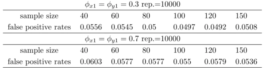
Table 2.1: Testing the equality of two AR(1) models at level 0.05 (difference sample size setting) φx1= φy1= 0.3 rep.=10000

sample size 40 60 80 100 120 150

false positive rates 0.0556 0.0545 0.05 0.0497 0.0492 0.0508 φx1= φy1= 0.7 rep.=10000

sample size 40 60 80 100 120 150

false positive rates 0.0603 0.0577 0.0577 0.055 0.0579 0.0536

2.4

A simulation study

In this section we conduct simulation studies to evaluate our testing results. In the first simulation study, we evaluate the performance of the confidence interval of AR(1) models basd on (2.6) in terms of their false positive rate. For our methods, the sample sizes of two time series that we want to compare may not equal, but we set the same for them in our simulation. We chose sample sizes as 40,60,80,100,120 and 150 and σε = 1. For each value of sample sizes, we generated 10000 data sets from the AR(1)

model with both φx1= φy1= 0.3 and φx1= φy1 = 0.7. Then we computed 95% CIs for

φx1− φy1. From Tables 2.1, we see that all of the false positive rates of each value of

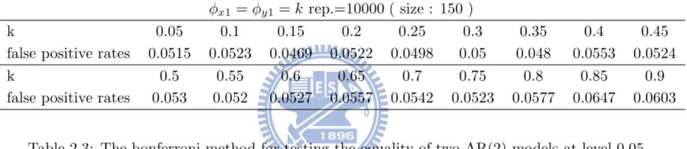
sample sizes are close to 0.05. Next, we set various paramaters of AR(1) model for the same sample size 150 in Table 2.2. Their false positive rates are also near to 0.05.

In the second simulation study, we consider the AR(2) models and their false positive rate. The false positive rates in Table 2.3 and 2.4 have no obvious difference for these two methods. It show that when the sample size is 150, the false positive rates are very close to 0.05. Therefore, if we want to compare two time series, the sample sizes of the model we fitted should not be less than 100.

Table 2.2: Testing the equality of two AR(1) models at level 0.05 (difference β setting) φx1= φy1= k rep.=10000 ( size : 150 )

k 0.05 0.1 0.15 0.2 0.25 0.3 0.35 0.4 0.45

false positive rates 0.0515 0.0523 0.0469 0.0522 0.0498 0.05 0.048 0.0553 0.0524

k 0.5 0.55 0.6 0.65 0.7 0.75 0.8 0.85 0.9

false positive rates 0.053 0.052 0.0527 0.0557 0.0542 0.0523 0.0577 0.0647 0.0603

Table 2.3: The bonferroni method for testing the equality of two AR(2) models at level 0.05 β

x= βy = (φy1, φy2)′= (0.3, 0.3)′ rep.=10000

sample size 40 60 80 100 150 200 300 500

false positive rates 0.0645 0.0601 0.0586 0.0563 0.0514 0.0513 0.0495 0.0496 Table 2.4: The Chisque method for testing the equality of two AR(2) models at level 0.05

β_x= β_y = (φy1, φy2)′= (0.3, 0.3)′ rep.=10000

sample size 40 60 80 100 150 200 300 500

3

A Test of Equality of RCA Models

3.1

Introduction

The first example for the random coefficient autoregressive (RCA) model was in-troduced and studied by Nicholls and Quinn (1982). They derived the necessary and sufficient condition for the process to be second-order stationary. In addition, they also discuss some properties and methods for the RCA model. We wrote the model RCA(1) as

Zt= rtZt−1+ εt (3.1)

rt = µr+ σrut,

where εt’s and ut’s are sequences of iid realizations from a distribution. And, εtand

ut are also independent. Since Wang and Ghosh (2002) defined the η = µ2r+ σ2r and

called η the stationary parameter for the RCA(1) model, the necessary and sufficient condition for the process is η < 1.

A generalized form of the RCA model was introduced by Hwang and Basawa (1998). The Markovian bilinear model, the random coefficient exponential autoregres-sive process and the RCA model all are special cases of it. A time series Yt is a

generalized random coefficient autoregressive (GRCA) process if

Yt = φ ′

where φt= (φt1, · · · ,φtp)′, Y (t − 1) = (Yt−1, · · · , Yt−p)′. In here, E      φt εt     =      φ 0     and Var      φt εt     =      Vφ σφε σ′ φε σε2     

where φ = (φ1, · · · , φp)′, Vφ= V ar(φt) is a (p × p) matrix, σφε=Cov(φt, εt) is a (p × 1)

vector, and σ2

ε= V ar(ε). Note that a GRCA process reduces to the RCA process by

setting σφε = 0.

Hwang and Basawa (1998) had deriven conditional least squares and weighted least squares estimators of the mean of the random vector. Their asymptotic properties and limit distributions had also been studied. Like ARMA models, we rarely see the discussions about the comparion of two time series from RCA models. Considering two time series xt and ytwhich both satisfy formula (3.2), in this chapter, we are interested

in testing the equality of φx and φy.

3.2

Basic Results

Although the conditional least-squares (LS) and weighted conditional least-squares (WLS) estimators of parameter in the general RCA model had been derived, the high order moment condition that assuming the fourth-order moment of the stationary dis-tribution of the series exists is not easy to be verified. In particular, since the limiting distributions of these estimators also depend on other nuisance parameters, the LS or WLS procedure cannot be directly used to test the hypotheses about φ.

gen-confidence intervals on φ. In their simulation results, using EL method, the coverage probabilities of the 95% confidence intervals were maintained at around 95% through-out, but LS and WLS method can not reach level 95% when sample size n = 50, 100, 300 and 500. Moreover, they also point out the empircal likelihood method is more accurate and robust than the normal approximation-based method.

Let φ0 denote the true parameter value for φ and Gt(φ) = YtY (t − 1) − Y (t −

1)Y′

(t − 1)φ. Then the log-empirical likelihood ratio is

l(φ) = 2 n X t=1 log(1 + λtGt(φ)), (3.3) where λ ∈R p _satisfies 1 n n X t=1 Gt(φ) 1 + λt_G t(φ) = 0.

Under appropriate conditions (see Zhao and Wang, 2011), l(φ0) converges to the

chi-square distribution with degrees of freedom p, i.e.

l(φ0) d

−

→ χ2(p) as n → ∞

Then, for 0 < α < 1, an asymptotic 100(1 − α)% confidence region of φ is given by

{φ ∈ ℜp : l(φ) ≤ χ2α(p)}

where χ2

3.3

Testing Methods

We consider two time series xt and yt which both are from RCA(p) models:

xt= φxtX(t − 1) + εxt

yt = φytY (t − 1) + εyt

We are interested in testing if φx and φy are equivalent. Let lx(φx) and ly(φy) be the

log empirical likelihood ratio of xtand yt, respectively. Note that the asymptotic

distri-butions of lx(φx) and ly(φy) both are chi-square distributions with degrees of freedom

p. This means that

lx(φx)−→ χd 2(p) as n → ∞

ly(φy) d

−

→ χ2(p) as n → ∞

We recall a random variate of the F-distribution arises as the ratio of two appropri-ately scaled chi-square variates. Therefore, for testing the null hypothesis H0 : φx = φy

against the alternative hypothsis H1 : φx 6= φx, the test statistic F and its asymptotic

distribution is F = lx(φx) ly(φy) d − → F (p, p) as n → ∞ (3.4)

We rejects H0 : l(φx) = l(φy) if F < Fα(p, p), where Fα(p, p) is the upper α-quantile

of the F distribution with parameters (p, p). Since the above foumla includes the ratio of functions lx and ly, we could not obtain the confidence region using this method

3.4

A simulation study

In the simulation study, the sample size is selected to be 150 through this section. Since the beta density function can have different shapes depending on the parameter values, we consider that rt are iid from the beta(a, b) distribution and (3.1) can be

written as Zt= rtZt−1+ εt, (3.5) where rt iid ∼ Beta(a, b), ε_t iid

∼ N(0, σ_ε), µ_r = E(r_t) and σ_r = V ar(r_t). Then, for any a,

b > 0, the stationary parameter is

η = µ2_r+ σ_r2 = ( a a + b) 2₊ ab (a + b + 1)(a + b)2 = ( a a + b) 2₍a + b + 1 a + b + 1) + ab (a + b + 1)(a + b)2 = a 3_{+ a}2_{b + a}2_{+ ab} (a + b + 1)(a + b)2 = a 3_{+ a}2_{b + a}2_{+ ab} a3_{+ 3a}2_{b + 3ab}2_{+ b}3 _{+ a}2 _{+ 2ab + b}2 = (a 3_{+ a}2_{b + a}2_{+ ab)} (a3_{+ a}2_{b + a}2_{+ ab) + 2a}2_{b + 3ab}2_{+ b}3_{+ ab + b}2.

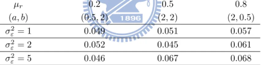
Since 2a2b + 3ab2+ b3+ ab + b2 > 0, the stationary condition (η < 1) is always satisfied. In this simulation, we set the pairs (a, b) as (0.5,2), (2,2) and (2,0.5). The corre-sponding µr is 0.2, 0.5 and 0.8, respectively. Table 3.1 shows the rejection rates such

that the type I error in our testing result is at level 0.05. The simulation replicants is 1000, and the rejection rates are very close 0.05 in difference parmaters setting.

Table 3.1: The EL method for testing the equality of two RCA(1) models at level 0.05 µr 0.2 0.5 0.8 (a, b) (0.5, 2) (2, 2) (2, 0.5) σ2 ε= 1 0.049 0.051 0.057 σ2 ε= 2 0.052 0.045 0.061 σ2 ε= 5 0.046 0.067 0.068

4

Application

In this chapter, we illustrate our testing method by a real data example. The data sets we use are the monthly sales of FamilyMart, President Chain Store and Poya in Taiwan. These data were obtained from Taiwan Economic Journal (TEJ), http://www.finasia.biz/ensite/.

First, we consider the data consists of 145 records for the monthly sales of Fami-lyMart and President Chain Store ranging from March 2000 to March 2012 presented in Figure 4.1, which show that the two time series are nonstationary. We take first differneces for both series in natural log scale. The sample autocorrelation and partial autocorrelation functions are also ploted in Figure 4.2 . Since the output in Figure 4.2 shows that the first differnece of the natural logarithms dies down very slowly at the seasonal level, we also take seasonal differneces with lag 12 for both series and denote them as Z1t and Z2t , t = 1, ..., n, respectively.

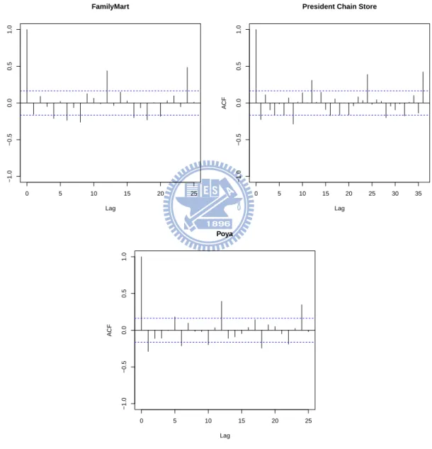
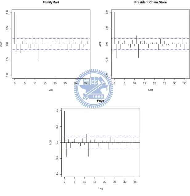
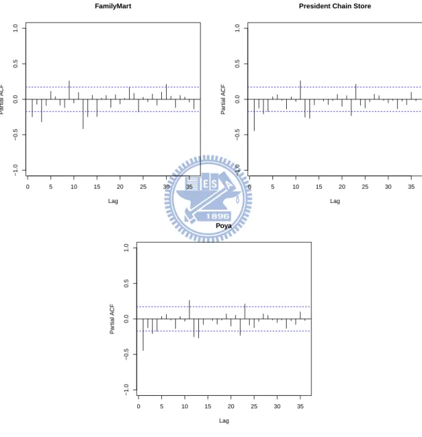
The ACF and PACF of the two series Z1t and Z2t are shown in Figure 4.3 and

4.4 which are used to identify a suitable model for the two time series. We determine the ARMA order of Z1t first. At seasonal level, the ACF and PACF of Z1t suggest

that we may consider first-order seasonal MA model with the yearly seasonal period MA(1)12 or second-order seasonal AR model with the yearly seasonal period AR(2)12

to fit seasonal part. Since the coefficient of MA(1)12 we estimated is very close to 1,

at lag 3 and the ACF dies down. We may fit an AR(3) model. Although the partial autocorelation at lag 9 is significant, it is hard to explain why the sales depend on the past ninth month.

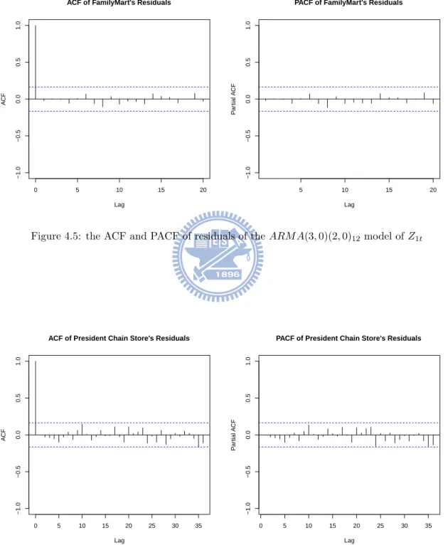
We combine the seasonal model and nonseasonal model above. This gives the overall model ARMA(3, 0)(2, 0)12for Z1t. Since the ACF and PACF of Z2t have similar

pattern for Z1t, we directly use the same model to fit Z2t. We can see that both residuls

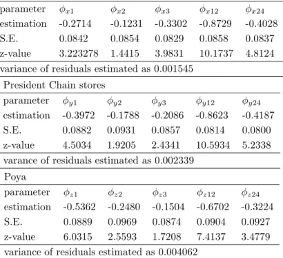
of fited models look like white noise and their ACF and PACF in Figure 4.5 and 4.6 have no spikes in any lag. Hence, we conclude that our models is adequate and the coefficients we estimated are given in Table 4.5.

We performe our methods to test equality of two models. The testing statistic is

χ2 = ( ˆβx− ˆβy) ′ V∗ −1 ( ˆβx− ˆβy) =                   −0.2714 −0.1231 −0.3302 −0.8729 −0.4028          −          −0.3972 −0.1788 −0.2086 −0.8623 −0.4187                   ′ V∗ −1                   −0.2714 −0.1231 −0.3302 −0.8729 −0.4028          −          −0.3972 −0.1788 −0.2086 −0.8623 −0.4187                   =          0.1258 0.0557 −0.1216 −0.0106 0.0159          ′         0.0149 0.0050 0.0011 −0.0014 −0.0024 0.0050 0.0160 0.0044 −0.0017 −0.0015 0_.0011 0_.0044 0_.0143 0_{.0000 −0.0003} −0.0014 −0.0017 0.0000 0.0140 0.0085 −0.0024 −0.0015 −0.0003 0.0085 0.0134          −₁         0.1258 0.0557 −0.1216 −0.0106 0.0159          = 2.602746

where V∗ =          0_.0071 0_.0019 0_{.0003 −0.0005 −0.0010} 0.0019 0.0073 0.0016 −0.0004 −0.0005 0.0003 0.0016 0.0069 0.0002 0.0000 −0.0005 −0.0004 0_.0002 0_.0074 0_.0044 −0.0010 −0.0005 0.0000 0.0044 0.0070          +          0_.0078 0_.0031 0_{.0008 −0.0009 −0.0014} 0.0031 0.0087 0.0028 −0.0013 −0.0010 0.0008 0.0028 0.0074 −0.0002 −0.0003 −0.0009 −0.0013 −0.0002 0_.0066 0_.0041 −0.0014 −0.0010 −0.0003 0.0041 0.0064          Since χ2 _{= 2.602746 <11.0705 = χ}2

0.05(5), we did not reject the equality of two series

under our model assumption.

On the other hand, we are also interested in the variation of FamilyMart’s and Poya’s monthly sales in the same periods that we analyzed above. We directly take log and differneces in seasonal and nonseasonal lag of Poya’s monthly sales and denote it by Z3t. The model ARMA(3, 0)(2, 0)12 is considered as well. We performe bonferroni

method and chi-square method for testing the equality of paramaters which we esti-mated to FamilyMart’s and Poya’s monthly sales. The chi-square statistic 11.60805 is larger than χ2

0.05(5). This means that there are significantly difference between

Fam-ilyMart’s and Poya’s relationships between past sales and future sales. However, the critical value by bonferroni approach is z1−0.05/(2∗5) = 2.575829 and z-value for the five

coefficirnt are 2.16, 0.97, 1.49, 1.63, 0.64. There are not any significantly difference between the parameters in two ARMA(3, 0)(2, 0)12 models by bonferroni approach.

Table 4.1: The 145 records for the monthly sales of FamilyMart 1176297 1203511 1298980 1341173 1448275 1412358 1377681 1420655 1324594 1370169 1424020 1257277 1393381 1401237 1493782 1561164 1700699 1742855 1557325 1606533 1496431 1630714 1603934 1625136 1699289 1743039 1897031 1958004 2022666 2000199 1857083 1883538 1736939 1817184 1823917 1757139 1842472 1889945 2034507 2115684 2290404 2231388 2170777 2152775 2047819 2052770 2192003 1972375 2126223 2143391 2357776 2346279 2525170 2551546 2356080 2331998 2213939 2248976 2186831 2172723 2263059 2364689 2434188 2273040 2627003 2703091 2646670 2635123 2736831 2640543 2738463 2338039 2270752 2493470 2694421 2783042 2740841 2692549 2542157 2670539 2408413 2414213 2416360 2502406 2555435 2551918 2728505 2698956 3029872 3344389 3081076 2937270 2753587 2818224 3006540 3026450 2921727 3081081 3274186 3159104 3456286 3470185 3228930 3221119 2952750 3033530 3228163 2899779 3036564 2956038 3258665 3212950 3632916 3679114 3434640 3541790 3171044 3154109 3184423 3260491 3325341 3268256 3717275 3632261 4003762 3960021 3704590 3783590 3547716 3566106 3495592 3308275 3507977 3796799 3927056 3892256 4186706 4203710 4444292 4411963 4145609 4107737 4523114 3898680 4269153

Table 4.2: The 145 records for the monthly sales of President Chain Store

4491115 4757277 4917705 5317334 5151417 4944261 5114518 4688220 4851881 5245460 4551829 5006136 4955858 5402798 5796654 6071025 6134253 5310996 5542568 5071628 5662084 5440804 5478789 5664451 5795443 6204563 6358800 6711169 6613039 6059449 6141493 5703570 5831072 5902463 5909544 5948880 6123298 6549613 6634948 7244164 7106254 6868259 6737832 6369917 6270463 7005126 6193627 6329060 6378422 6926771 6892067 7314727 7363984 6762306 6739042 6445986 6585437 6427478 6693389 6636050 6874298 8426333 9389209 10189078 8048829 7797608 7920930 7751074 7486858 7957398 6906009 7772104 8182944 8531847 8088966 9657812 9241675 8694701 8637923 8097559 8187449 7775909 8573222 8272678 8087873 9447797 9192908 9296334 8561123 8253002 8471859 7997619 8403231 8286532 8240892 7955810 7937409 8451530 8620256 9401185 9279031 8521024 8904654 8407819 8185085 8678734 7479726 7982511 8173621 9085255 8521446 8795788 8813036 8322949 8602572 8440369 8860415 8761825 8861694 9267065 8895036 9686463 9495227 10289154 10189891 10040908 10105227 9341217 9730864 9336890 9540881 9406303 9534967 10243258 10393956 10806588 10657507 10811993 10941694 10379517 10659172 11675088 9969214 10604789

Table 4.3: The 145 records for the monthly sales of Poya 134572 139882 151795 142373 169890 158217 156978 144326 131484 146331 159908 154044 167596 164856 159300 160481 175428 174350 178467 171466 159049 170817 153637 154914 158808 159861 169925 159645 166328 190791 228079 203493 191163 203540 217475 209811 227167 202533 226091 213989 241005 239018 245058 239038 217248 260849 266234 237624 220658 225923 245033 231372 239919 280470 289460 279621 240378 284378 271904 270610 255527 256112 265460 262181 278458 275864 272014 281022 270523 319695 295752 269613 263292 264167 276487 272641 288919 298156 331839 296026 307825 352557 309917 338401 319048 312168 338692 317888 359587 366206 402671 363113 347163 395244 380332 416281 374001 376488 382949 382992 391630 477309 436935 443974 423617 448455 524183 415991 405746 401773 451212 412836 474039 511685 508552 494973 460700 556776 523646 508097 490038 471239 499398 468760 534932 550774 525182 516074 465039 538118 546607 513171 457284 465630 469685 513494 564373 563342 566643 538218 486194 571026 619879 511171 486322

Table 4.5: The estimation of the parimaters of ARM A(3, 0)(2, 0)12model

FamilyMart

parameter φx1 φx2 φx3 φx12 φx24

estimation -0.2714 -0.1231 -0.3302 -0.8729 -0.4028 S.E. 0.0842 0.0854 0.0829 0.0858 0.0837 z-value 3.223278 1.4415 3.9831 10.1737 4.8124 variance of residuals estimated as 0.001545

President Chain stores

parameter φy1 φy2 φy3 φy12 φy24

estimation -0.3972 -0.1788 -0.2086 -0.8623 -0.4187 S.E. 0.0882 0.0931 0.0857 0.0814 0.0800 z-value 4.5034 1.9205 2.4341 10.5934 5.2338 varance of residuals estimated as 0.002339

Poya

parameter φz1 φz2 φz3 φz12 φz24

estimation -0.5362 -0.2480 -0.1504 -0.6702 -0.3224 S.E. 0.0889 0.0969 0.0874 0.0904 0.0927 z-value 6.0315 2.5593 1.7208 7.4137 3.4779 variance of residuals estimated as 0.004062

FamilyMart’s and President Chain Store’s Sales

Months

Sales (Thousand Dollars)

FamilyMart

President Chain Store

Mar−00 Mar−02 Mar−04 Mar−06 Mar−08 Mar−10 Mar−12

1e+06 4e+06 8e+06 1.2e+07 Poya’s Sales Months

Sales (Thousand Dollars)

Mar−00 Mar−02 Mar−04 Mar−06 Mar−08 Mar−10 Mar−12

2e+05

3e+05

4e+05

5e+05

6e+05

0 5 10 15 20 25 −1.0 −0.5 0.0 0.5 1.0 Lag A CF FamilyMart 0 5 10 15 20 25 30 35 −1.0 −0.5 0.0 0.5 1.0 Lag A CF

President Chain Store

0 5 10 15 20 25 −1.0 −0.5 0.0 0.5 1.0 Lag A CF Poya

0 5 10 15 20 25 30 35 −1.0 −0.5 0.0 0.5 1.0 Lag A CF FamilyMart 0 5 10 15 20 25 30 35 −1.0 −0.5 0.0 0.5 1.0 Lag A CF

President Chain Store

0 5 10 15 20 25 30 35 −1.0 −0.5 0.0 0.5 1.0 Lag A CF Poya

0 5 10 15 20 25 30 35 −1.0 −0.5 0.0 0.5 1.0 Lag P ar tial A CF FamilyMart 0 5 10 15 20 25 30 35 −1.0 −0.5 0.0 0.5 1.0 Lag P ar tial A CF

President Chain Store

0 5 10 15 20 25 30 35 −1.0 −0.5 0.0 0.5 1.0 Lag P ar tial A CF Poya

0 5 10 15 20 −1.0 −0.5 0.0 0.5 1.0 Lag A CF

ACF of FamilyMart’s Residuals

5 10 15 20 −1.0 −0.5 0.0 0.5 1.0 Lag P ar tial A CF

PACF of FamilyMart’s Residuals

Figure 4.5: the ACF and PACF of residuals of the ARM A(3, 0)(2, 0)12model of Z1t

0 5 10 15 20 25 30 35 −1.0 −0.5 0.0 0.5 1.0 Lag A CF

ACF of President Chain Store’s Residuals

0 5 10 15 20 25 30 35 −1.0 −0.5 0.0 0.5 1.0 Lag P ar tial A CF

PACF of President Chain Store’s Residuals

0 5 10 15 20 25 30 35 −1.0 −0.5 0.0 0.5 1.0 Lag A CF

ACF of Poya’s Residuals

0 5 10 15 20 25 30 35 −1.0 −0.5 0.0 0.5 1.0 Lag P ar tial A CF

PACF of Poya’s Residuals

5

Conclusions

In this thesis, we study and review the literature on estimation and inference for ARMA models based on MLE method. For comparing time series, we proposed an approach to test the equality of the parameters estimated from two time series. We also presente the Bonferroni approach for multiple testing. In addition to the classical ARMA based methods to compare two time series, we considered the RCA models as well. We performe the empirical likelihood estimation for both RCA models, and then test equality of their means of random coefficients by the F distribution. We also considere beta distribution for the random coefficient of the RCA(1) model and show that the stationary condition is always satisfied. For testing for ARMA models or RCA models, our simulations verify the testing results can attain a desired level mostly. Finally, we practice our methods for real data. The data consists of three companies’ monthly sales, namely, FamilyMart, President Chain Store and Poya. In our analysis, we conclude that there are significantly difference between FamilyMart’s and Poya’s sales behavior.

Bibliography

[1] H. Abdi. Bonferroni and sidak corrections for multiple comparisons. Encyclopedia of Measurement and Statistics, 1:103–107, 2007.

[2] N.A. Abdullah, I. Mohamed, S. Peiris, and N.A. Azizan. A new iterative pro-cedure for estimation of rca parameters based on estimating functions. Applied Mathematical Sciences, 5(4):193–202, 2011.

[3] C. Alberola-L´opez and M. Mart´ın-Fern´andez. A simple test of equality of time series. Signal processing, 83(6):1343–1348, 2003.

[4] A. Aue, L. Horv´ath, and J. Steinebach. Estimation in random coefficient autore-gressive models. Journal of Time Series Analysis, 27(1):61–76, 2006.

[5] P.J. Brockwell and R.A. Davis. Time series: theory and methods. springer Verlag, (2009).

[6] J. Durbin. Estimation of parameters in time-series regression models. Journal of the Royal Statistical Society. Series B (Methodological), 22:139–153, 1960.

[7] E.P. George. Time series analysis: Forecasting and control. Holden-D., (1970). [8] S.Y. Hwang and I.V. Basawa. Parameter estimation for generalized random

co-efficient autoregressive processes. Journal of statistical planning and inference, 68(2):323–337, 1998.

[9] D.F. Nicholls. The box-jenkins approach to random coefficient autoregressive mod-elling. Journal of Applied Probability, pages 231–240, 1986.

[10] D.F. Nicholls and B.G. Quinn. Random coefficient autoregressive models: an in-troduction. Springer.

[11] R.H. Shumway and D.S. Stoffer. Time series analysis and its applications. Springer Verlag, (2000).

[12] D. Wang. Frequentist and bayesian analysis of random coefficient autoregressive models. North Carolina State University, Ph.D, 2003.

[13] Z.W. Zhao and D.H. Wang. Statistical inference for generalized random coefficient autoregressive model. Mathematical and Computer Modelling, 2011.