國 立 交 通 大 學
電信工程學系碩士班
碩 士 論 文
手持式數位電視天線之微小化設計
Miniaturization of DVB-H Handset Antennas
研 究 生:許志瑋
指導教授:唐震寰 教授
手持式數位電視天線之微小化設計
Miniaturization of DVB-H Handset Antennas
研 究 生:許志瑋 Student:Chih-Wei Hsu
指導教授:唐震寰 教授 Advisor:Jenn-Hwan Tarng
國 立 交 通 大 學
電 信 工 程 學 系 碩 士 班
碩 士 論 文
A ThesisSubmitted to Department of Communication Engineering College of Electrical Engineering and Computer Science
National Chiao Tung University in Partial Fulfillment of the Requirements
for the Degree of Master
in
Communication Engineering
June 2007
Hsinchu, Taiwan, Republic of China
手持式數位電視天線之微小化設計
研究生:許志瑋 指導教授:唐震寰 教授
國立交通大學
電信工程學系 碩士班
摘要
寬頻、小尺寸、天線場型及增益都是設計天線時重要的考量因子。然而這些因子 彼此之間可能會相互衝突,所以設計時必須適當的折衝與取捨。本論文設計兩個 可以應用於手持式數位電視天線,分別應用蝴蝶結單極天線結構與冪次函數曲線 結構製做天線,前者藉由將接地面圍繞天線提出半蝴蝶結的天線架構達到微小化 及寬頻,後者應用冪次函數曲線增加前者頻寬以滿足手持式數位電視的規範。量 測結果,該天線的操作頻帶涵蓋 470 MHz 至 800 MHz。該天線為平面結構減低製 作上的困難,且該天線面積小於文獻中其他設計於手持式數位電視頻段的體積。 輻射場型經由數值模擬顯示,皆具有近似單指向的(Omni-directional)輻射場 型,且具有合理之天線增益,分別介於 2.2 dBi 至 3.5 dBi 之間。Miniaturization of DVB-H Handset Antennas
Student:Chich-Wei Hsu Advisor:Dr. Jenn-Hwan Tarng
Department of Communication Engineering
National Chiao Tung University
Abstract
Broadband, size reduction, radiation pattern, and antenna gain are the major issues to be considered. It is well-known that these issues are trade-offs one another. In the thesis, by applying half-bow-tie monopole antenna and x to the power of N curved line structure, two antenna prototypes for DVB-H are proposed. With the help of ground plane surrounding the antenna, a half-bow-tie monopole antenna is proposed to increase the bandwidth. To broaden bandwidth, boundaries of No.1 antenna are changed and become a curved line. The curved line is described by a x to the power of N. The simulated and measured results confirmed that the proposed antenna can operates at 470 MHz to 800 MHz bands. The antenna not only has a simple planar structure but also yields the smallest antenna area. Moreover, the antenna has a nearly omni-directional radiation pattern and a reasonable peak gain of 2.25 dBi to 3.74 dBi.
誌
謝
在碩士研究的這二年歲月,首先要感謝的是我的指導教授 唐震寰教授並致 上我最誠摯的謝意。感謝老師在專業的通訊領域中,給予我不斷的指導與鼓勵, 並賦予了實驗室豐富的研究資源與環境,使得這篇碩士論文能夠順利完成。 其次,要感謝波散射與傳播實驗室的學長們—鄭士杰學長、劉文舜學長、莊 秉文學長、宜興學長、和穆學長、孟勳學長、舜升學長、懷文學長在研究上的幫 助與意見,讓我獲益良多。感謝實驗室的同學—奕慶、豐吉、育正、思云、蓓縝 等在課業及研究上的互相砥礪與切磋,以及生活上的多彩多姿。感謝學弟們—雅 仲、俊諺等,讓實驗室在嚴肅的研究氣氛中增添了許多歡樂,有了你們,更加豐 富了我這二年的研究生生活。另外,也要感謝助理—梁麗君小姐,在生活上的協 助和籌劃每次的美食聚餐饗宴。 最後,要感謝的就是我最親愛的家人,由於他們在我求學過程中,一路陪伴 著我,給予我最溫馨的關懷與鼓勵,讓我在人生的過程裡得到快樂,更讓我可以 專心於研究工作中而毫無後顧之憂。 鑒此,謹以此篇論文獻給所有關心我的每一個人。 許志瑋 誌予 九十六年六月CONTENTS
ABSTRACT (CHINESE)
………..……ⅠABSTRACT (ENGLISH)……….
ⅡACKNOWLEDGEMENT………....Ⅲ
LIST OF TABLES………...Ⅵ
LIST OF FIGURES………
ⅦCHAPTER 1
INTRODUCTION
11.1 Background and Problems………..……1
1.2 Related Works………...3
1.3 Thesis Organization……….4
CHAPTER 2 BROADBAND ANTENNA BASICS
52.1 Fundamental Parameters of Antennas……….…………..5
2.1.1 Reflection coefficient………...………5
2.1.2 Quality factor, bandwidth, and efficiency………....6
2.1.3 Radiation pattern………...…8
2.1.4 Directivity and gain………...……10
2.2 Broadband Antennas……….12
2.2.1 Traveling-wave antenna………..………...………12
CHAPTER 3 THE PROPOSED DVB-H ANTENNA
213.1 Design Flow of DVB-H Antenna….………...….…21
3.1.1 Problem analysis – size reduction……….…….22
3.1.2 Broaden the impedance bandwidth………...23
3.2 Proposed Antenna Prototype No.1 ………...…….……….….….23
3.2.1 Numerical analysis of antenna prototype no.1 ……….…25
3.2.2 The advantage of antenna prototype no.1 ………..……..30
3.3 Proposed Antenna Prototype No.2 ………...………….….….31
3.3.1 Numerical analysis of antenna prototype no.2 ……….…31
3.3.2 Comparison between computed and measured results …….…..41
CHAPTER 4
CONCLUSION
45List of Tables
Table 1.1 DVB-T Broadcaster in Taiwan………..….2 Table 3.1 Size, bandwidth and gain comparisons between proposed antenna
prototype No.1 and other published DVB-H antennas……….…30 Table 4.2 The peak gain and average gain of the proposed antenna prototype
No.2………40 Table 4.3 Size, bandwidth and gain comparisons between our works and other
List of Figures
Figure 1.1 Frequency allocation for DVB-H channels………....2
Figure 2.1 Radiation pattern from an ideal dipole………...8
Figure 2.2 E-plane radiation pattern polar plot of Eθ or H ………....8 φ Figure 2.3 Principal E-plane and H-plane patterns for a pyramidal horn antenna………9
Figure 2.4 Traveling-wave long wire antenna………14
Figure 2.5 Unidirectional and bidirectional V antennas………15
Figure 2.6 Terminated V antennas………16
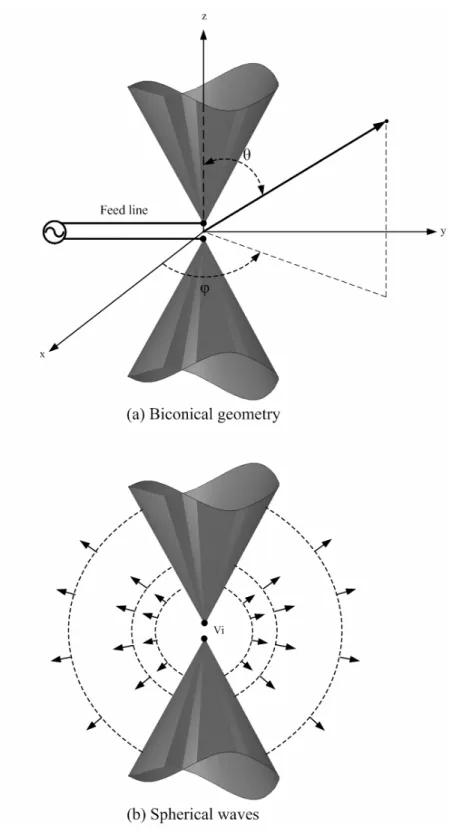
Figure 2.7 Biconical antenna geometry and radiated spherical waves…………17
Figure 2.8 Electric and magnetic fields, and associated voltages and currents, for a biconical antenna………18
Figure 2.9 Finite biconical antenna……….…19
Figure 2.10 Computed input impedance of a conical monopole with flare angle versus monopole height (a) real part (b) imaginary part………..20
Figure 3.1 The design flow of the DVB-H antenna………22
Figure 3.2 The proposed DVB-H antenna prototype No.1………...…24
Figure 3.3 Front view of the proposed DVB-H antenna prototype No.1 for a clamshell mobile phone……….……24
Figure 3.4 Computed return loss versus frequency by varying α………25
Figure 3.5 Radiation patterns of DVB-H antenna prototype at 500 MHz, (a) x-z plane ,(b) y-z plane ,and (c) x-y plane.………26
Figure 3.6 Radiation patterns of DVB-H antenna prototype at 600 MHz(a) x-z plane ,(b) y-z plane ,and (c) x-y plane.………27
Figure 3.7 Radiation patterns of DVB-H antenna prototype at 700 MHz(a) x-z plane ,(b) y-z plane ,and (c) x-y plane.………28
Figure 3.8 Computed antenna gain verse frequency………..29 Figure 3.9 The proposed DVB-H antenna prototype No.2. (The curved line C is plotted when N=18.)……….…………...….31
Figure 3.10 Computed return loss versus frequency by varying N………...…..…32
Figure 3.11 Computed return loss versus frequency by varying gap width (g)...…33
Figure 3.12 Computed return loss versus frequency by varying tilting β.………...33
Figure 3.13 Radiation patterns of proposed DVB-H antenna at 470 MHz(a) x-z plane ,(b) y-z plane ,and (c) x-y plane.………34 Figure 3.14 Radiation patterns of proposed DVB-H antenna at 500 MHz(a) x-z
plane ,(b) y-z plane ,and (c) x-y plane.………35 Figure 3.15 Radiation patterns of proposed DVB-H antenna at 550 MHz(a) x-z
plane ,(b) y-z plane ,and (c) x-y plane.……….……36 Figure 3.16 Radiation patterns of proposed DVB-H antenna at 600 MHz(a) x-z
plane ,(b) y-z plane ,and (c) x-y plane.………37 Figure 3.17 Radiation patterns of proposed DVB-H antenna at 700 MHz(a) x-z
plane ,(b) y-z plane ,and (c) x-y plane.………38 Figure 3.18 Radiation patterns of proposed DVB-H antenna at 800 MHz(a) x-z
plane ,(b) y-z plane ,and (c) x-y plane.………39 Figure 3.19 Computed antenna gain verse frequency………..……40 Figure 3.20 Computed and measured return loss versus frequency………41 Figure 3.21 Measured Radiation patterns of proposed DVB-H antenna at 750MHz (a) x-z plane, (b) y-z plane, and (c) x-y plane.………42 Figure 3.22 Measured Radiation patterns of proposed DVB-H antenna at 800MHz (a) x-z plane, (b) y-z plane, and (c) x-y plane.………43
CHAPTER 1 INTRODUCTION
CHAPTER 1 INTRODUCTION
1.1 Background and Problems
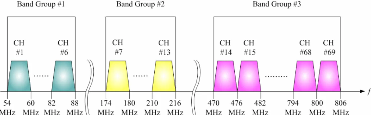
DVB-H (Digital Video Broadcasting - Handheld) is the digital broadcast standard for transmitting broadcast content to handheld terminal devices. DVB-H is based on the DVB-T standard for digital terrestrial television but tailored to the special requirements of pocket-size applications. The Federal Communication Commission (FCC) has recently approved the 54MHz to 88MHz, 174MHz to 216MHz, and 470MHz to 806 MHz bands for DVB-H deployment as shown in Figure 1.1, which are the same as the bands of DVB-T. In general, the DVB-H antennas operate in UHF IV and V (470-806 MHz, channels 14 to 69 [1]).
Since the quarter-wavelength of DVB-H bands (about 10-16 cm) is too large compared with the pocket-size, their antenna sizes need to be reduced to accommodated in a handheld device. It is well known that miniaturized antenna size, bandwidth, and reasonable antenna gain are trade-off with one another. The major challenge in DVB-H
CHAPTER 1 INTRODUCTION
antenna design is to provide an internal antenna that is small in size whilst maintaining the impedance bandwidth and reasonable antenna gain as required by the specifications.
Figure 1.1 Frequency allocation for DVB-H channels
Broadcaster Channel Number Frequency(MHz) 24 533 CTV 25 539 26 545 PTS 27 551 28 557 FTV 29 564 31 575 TTV 32 581 34 593 CTS 35 599
CHAPTER 1 INTRODUCTION
1.2 Related Works
In mobile communication systems, wide impedance bandwidth, miniaturized dimensions, and reasonable antenna gain are the critical requirements due to the highly competitive market environment and limitation in device dimensions. For DVB-H, there are only few studies proposed [2]-[6].
By using a compact coupling element structure, it is possible to reduce the size of an antenna element. The matching of the antenna is achieved with a dual-resonant lumped-element matching circuit [2]. It is noted that the impedance bandwidth of this tunable antenna is 470-702 MHz with return loss less than -1.25 dB, which is not a good performance criterion, the author claims that the DVB-H antenna is used in reception only, a loose matching criterion is acceptable.
A planar DTV receiving antenna for laptop applications is constructed by a bow-tie structure provides 480-742 MHz with return loss less than -7.4dB [3]. The antenna is cut by three narrow slits in the portion near the feeding point to achieve a compact, which extends the resonant path and makes the antenna size compact. By using the bow-tie structure, the impedance matching of the proposed antenna can be greatly improved.
By bending a flat metal-plate into U-shaped structure, a internal DTV receiving antenna for laptop applications is constructed provides 470-780 MHz with return loss less than -7.4dB [4]. The U-shaped structure, given the wide width, the antenna can provide broadband operation.
Although adding an external matching circuit can reduce antenna size, but treat the antenna as an input impedance can only provide a narrow impedance bandwidth with a common criterion. By bending a flat metal-plate into U-shaped or L-shaped structure can provide a broadband operation, but its fabrication is difficult that the
CHAPTER 1 INTRODUCTION
production cost is high. Inserting slits into antenna structure is a popular way for size reduction, but the antenna gain is also diminished. In this thesis, we focus on a compact DVB-H internal antenna solution for mobile phone. The planar antenna structure is chosen for easy fabrication.
1.3 Thesis Organization
The thesis is organized into five chapters including the introduction. Chapter 2 presents the broadband antenna basics, its metrics and some popular broadband antenna topologies. Chapter 3 discusses antenna design tool and simulation setup of the tool. In chapter 4, the simulation and measurement of proposed DVB-H antenna. Chapter 5 concludes the thesis and improvements are suggested for future work.
CHAPTER 2 BROADBAND ANTENNA BASICS
CHAPTER 2 BROADBAND ATNENNA BASICS
An antenna is defined by Webster’s Dictionary as “a usually metallic devise for radiating or receiving radio waves.” The IEEE Standard Definition of Terms for Antennas (IEEE Std 145-1983) defines the antenna or aerial as “a means for radiating or receiving radio waves.” In other words the antenna is the transitional structure between free-space and a guiding device. In this chapter, we introduce the parameters used to evaluate antennas and then briefly discuss some forms of the various antenna types.
2.1 Fundamental Parameters of Antenna
2.1.1
Reflection Coefficient
The reflection coefficient is the ratio of the amplitude of the reflected wave to the amplitude of the incident wave. In particular, at a discontinuity in a transmission line, it is the complex ratio of the electric field strength of the reflected wave to that of the
CHAPTER 2 BROADBAND ANTENNA BASICS
incident wave. The reflection coefficient is given by the equations below
0 0 Z Z Z Z L L + − = Γ (2-1) where Z is the impedance toward the source, 0 ZL is the impedance toward the load: When the load is mismatched not all of the power from the generator is delivered to the load. This “loss” is called return loss (RL), and is defined (in dB) as
Γ −
= 20log
RL dB (2-2) Due to the reflection, a voltage standing wave is created along the line, so a measure of the mismatch of a line, called the voltage standing wave ratio
Γ − Γ + = = 1 1 min max V V VSWR (2-3)
2.1.2
Quality Factor, Bandwidth, and Efficiency
The quality factor, bandwidth, and efficiency are antenna figures-of-merit, which are interrelated, and there is no complete freedom to independently optimize each one. Therefore there is always a trade-off between them in arriving at an optimum antenna performance. There is a desire to optimize one of them while reducing the performance of the other.
The quality factor is representative of the antenna losses. Typically there are radiation, conduction (ohmic), dielectric and surface wave losses. Therefore the total quality factor Q is influenced by all of these losses and is written as t
sw d c rad t Q Q Q Q Q 1 1 1 1 1 = + + + (2-4) where t
Q = total quality factor
rad
Q = quality factor due to radiation losses
c
CHAPTER 2 BROADBAND ANTENNA BASICS
d
Q = quality factor due to dielectric losses
sw
Q = quality factor due to surface waves
For very thin substrates, the losses due to surface waves are very small and can be neglected. However, for thicker substrates they need to be taken into account. For very thin substrates (h<<λ0) of arbitrary shape, there are approximate formulas to represent
the quality factors of the various losses. These can be expressed as
μσ πf h Qc = (2-5) δ tan 1 = d Q (2-6) K l hG Q t r rad / 2 ∈ = ω (2-7)
where tanδ is the loss tangent of the substrate material, σ is the conductivity of the conductors associated with the patch and ground plane, Gt/ is the total conductance l
per unit length of the radiating aperture. For a rectangular aperture operating in the dominant TM010x mode 4 l K = (2-8) W G l G rad t/ = (2-9)
The Grad is inversely proportional to the height of the substrate, and very thin substrates is usually the dominant factor. The fractional bandwidth of the antenna is inversely proportional to the Q of the antenna, and it can be expressed as t
VSWR Q VSWR Q f f t t 1 1 0 − = = Δ (2-10) In general bandwidth is proportional to the volume, which for a rectangular microstrip antenna at a constant resonant frequency. Therefore the bandwidth is inversely proportional to the square root of the dielectric constant of the substrate, and the bandwidth increases as the substrate height increases.
CHAPTER 2 BROADBAND ANTENNA BASICS
2.1.3
Radiation Pattern
A radiation pattern is a mathematical function or a graphical representation of the radiation properties of the antenna as a function. We have seen that the radiation fields form a transmitting antenna vary inversely with distance. The variation with observation angles
( )
φ,θ depends on the antenna.Radiation patterns can be understood by examining the ideal dipole. The fields radiated from an ideal dipole are shown in Figure 2.1 over the surface of a sphere of radius r that that is the far field. The angular variation of E and θ H over the φ
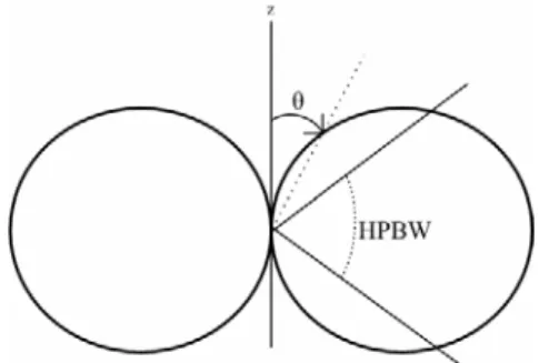
sphere is sinθ. To find the points where the pattern achieves its half-power, relative to the maximum value of the pattern, referred to as HPBW and illustrated in Figure 2.2.
Figure 2.1 Radiation pattern from an ideal dipole
CHAPTER 2 BROADBAND ANTENNA BASICS
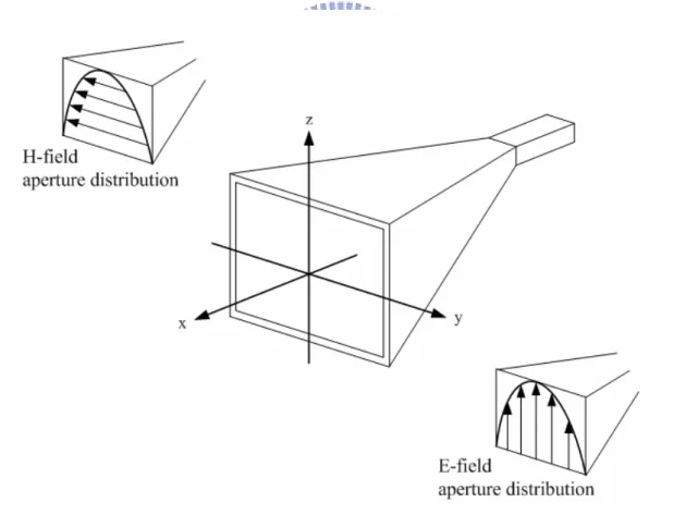
For a linearly polarized antenna, performance is often describe in terms of its principal E-plane and H-plane patterns. The E-plane is defined as “the plane containing the electric-field vector and the direction of maximum radiation,” and the H-plane as “the plane containing the magnetic-field vector and the direction of maximum radiation.” Although it is very difficult to illustrate the principal patterns without considering a specific example, it is the usual practice to orient most antennas so that at least on of the principal plane patterns coincide with one of the geometrical principal planes. An illustration is shown is Figure 2.3. For this example, the x-z plane (φ=0) is the principal E-plane and the x-y plane (θ =π /2) is the principal H-plane. The omnidirectional pattern of Figure 2.4 has an infinite of principal E-planes (φ = ) and φc one principal H-plane (θ =π/2)
CHAPTER 2 BROADBAND ANTENNA BASICS
2.1.4
Directivity and Gain
One very important description of an antenna is how much it concentrates energy in one direction in preference to radiation in other directions. This characteristic of an antenna is called its directivity and is equal to its power gain if the antenna is 100% efficient. Usually, power gain is expressed relative to a reference such as an isotropic radiator or half-wavelength dipole.
Directivity can be written as D=4πUm/P. Comparing this with (2-27), we see that the only difference between maximum gain and directivity is the power value used. Directivity can be viewed as the gain as antenna would have if all input power appeared as radiated power; that is, Pin = . Gain reflects the fact that real antennas do not P
behave in this fashion and some of the input power is lost on the antenna. The portion of input power P that does not appear as radiated power is absorbed on the antenna and in
nearby structures. This prompts us to define radiation efficiency er as
in r P P e = (2-28) Using (2-27) in (2-28) gives
( )
θ,φ 4π( )
θ,φ( )
θ,φ e D( )
θ,φ U U e P U e G r ave r r = = = (2-29)Similarly, for maximum gain
D e
G= r (2-30)
Since gain is a power ration it can be calculated in decibels as follows
G
GdB =10log (2-31)
Similarly for directivity,
D
DdB =10log (2-32)
For example, the directivity in decibels of an ideal dipole is 76 . 1 5 . 1 log 10 = = dB D dB ideal dipole (2-33)
CHAPTER 2 BROADBAND ANTENNA BASICS
half-wave dipole. The directivity of a half-wave dipole is 1.64, or 2.15 dB. Gain relative to a half-wave dipole carries the units of dBd. The unit dBi is often used instead of dB to emphasize that an isotropic antenna is the reference. In addition, the term absolute gain is sometimes used. As a numerical example, consider an antenna with a gain of 6.1 dB; its gain can be written in the following ways:
=
CHAPTER 2 BROADBAND ANTENNA BASICS
2.2
Broadband Antennas
In many applications, an antenna must operate effectively over a wide range of frequencies. An antenna with wide bandwidth is referred to as a broadband antenna. Bandwidth is computed in one of two ways. Let f and U fL be the upper and lower frequencies of operation for which satisfactory performance is obtained. The center frequency is denoted as f . Then bandwidth as a percent of the center frequency C BP
is % 100 × − = C L U P f f f B (2-35) Bandwidth is also defined as a ratio Br by
L U r f f B = (2-36) The definition of a broadband antenna is somewhat arbitrary and depends on the particular antenna, but we shall adopt a working definition. If the impedance and the pattern of an antenna do not change significantly over about an octave ( =2
L U
f f
) or more, we will classify it as a broadband antenna.
2.21
Traveling-wave Antenna
The wave traveling outward from the feed point to the end of the wire is reflected, setting up a standing-wave-type current distribution. The expression for the current on the top half of the dipole that can be written as
( L )
(
j z j z)
j m m e e e j I z L I β ⎥= β −β − +β ⎦ ⎤ ⎢ ⎣ ⎡ ⎟ ⎠ ⎞ ⎜ ⎝ ⎛ − /2 2 2 sin (2-37) If the reflected wave is not strongly present on an antenna, it is referred to as a traveling-wave antenna. A traveling-wave antenna acts as a guiding structure for traveling waves, whereas a resonant antenna supports standing waves. Traveling waves can be created by using matched loads at the ends to prevent reflections.CHAPTER 2 BROADBAND ANTENNA BASICS
The simplest traveling-wave wire antenna is a straight wire carrying a pure traveling wave, referred to as the traveling-wave long wire antenna. A long wire is one that is greater than one-half wavelength long. The traveling-wave long wire is shown in Figure 2.4 with a matched load RL to prevent reflections from the wire end. We shall make several simplifying assumptions that permit pattern calculation that do not differ greatly from real performance. First, the ground plane effects will be ignored and we will assume that the antenna operates in free space. A traveling-wave long wire operated in the presence of an imperfect ground plane is called a wave antenna. Second, the detail of the feed are assumed to be unimportant. In figure 2.4, the long wire is shown being fed from a coaxial transmission line as one practical method. The vertical section of length d is assumed not to radiate, which is approximately true for d <<L. Finally, we assume that the radiative and ohmic losses along the wire are small. When attenuation is neglected, the current amplitude is constant and the phase velocity is that of free space. We can write
jkz m t z I e
I ( )= − (2-38) which represents an unattenuated traveling wave propagating in the +z-direction with the phase constant k of free space.
The current of (2-38) is that of a uniform line source with a linear phase constant of
k
k0 =− . It is convenient to introduce an angle θ0 such that k0 =−kcosθ0, so the pattern factor maximum radiation angle is θ0 =0o, which implies an endfire pattern. The complete radiation pattern is
(
)(
)
[
]
(
)(
θ)
θ θ θ cos 1 2 / cos 1 2 / sin sin ) ( − − = kL kL K F (2-39) where K is a normalization constant that depends on the length L .CHAPTER 2 BROADBAND ANTENNA BASICS
Figure 2.4 Traveling-wave long wire antenna
One very particular array of long wires is the vee antenna formed by using two wires each with one of its ends connected to a feed line as shown in Figure 2.5(a). in most applications, the plane formed by the legs of the vee is parallel to the ground leading to a horizontal vee array whose principal polarization to the ground and the plane of the vee.
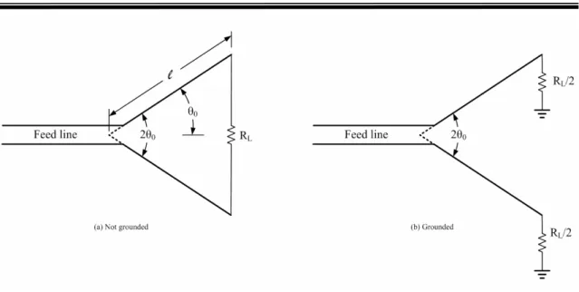
Most vee antennas are symmetrical (θ1=θ2 =θ0 and l1 =l2 =l ). Also vee antennas can be designed to have unidirectional or bidirectional radiation patterns, as shown in Figures 2.5 (b) and (c), respectively. To achieve the unidirectional characteristics, the wires of the vee antenna must be nonresonant which can be accomplished by minimizing if not completely eliminating reflections from the ends of the wire. The reflected waves can be reduced by making the inclined wires of the vee relatively thick. In theory, the reflections can be eliminated by properly terminating the open ends of the vee leading to a purely traveling wave antenna. One way of terminating the vee antenna will be to attach a load, usually a resistor equal in value to the open end characteristic impedance of the vee-wire transmission line, as shown in Figure 2.6(a). The terminating resistance can also be divided in half and each half connected to the ground leading to the termination of Figure 2.6(b). If the length of each leg of the vee is very long, there will be sufficient leakage of the field along each leg that when the wave reaches the end of the vee it will be sufficiently reduced that there
CHAPTER 2 BROADBAND ANTENNA BASICS
will not necessarily be a need for a termination.
The patterns of the individual wires of the vee antenna are conical in form and are inclined at an angle from their corresponding axes. The angle of inclination is determined by the length of each wire. For the patterns of each leg of a symmetrical vee antenna to add in the direction of the line bisecting the angle of the vee and to form one major lobe, the total included angle 2θ0 of the vee should equal to 2θm, which is
twice the angle that the cone of maximum radiation of each wire makes with its axis. When the is done beams 2 and 3 of Figure 2.5(b) are aligned and add constructively.
Similarly for Figure 2.5(c), beams 2 and 3 are aligned and add constructively in the forward direction, while beams 5 and 8 are aligned and add constructively in the backward direction.
CHAPTER 2 BROADBAND ANTENNA BASICS
Figure 2.6 Terminated V antennas
2.2.2
Biconical Antenna
One simple configuration that can be used to achieve broadband characteristics is the biconical antenna formed by placing two cones of infinite extent together, as shown in Figure 2.7(a). This can be thought to represent a uniformly tapered transmission line. The application of a voltage V at the input terminals will produce outgoing spherical i
waves, as shown in Figure 2.7(b), which in turn produce at any point (r,θ =θC,φ) a current I along the surface of the cone and voltage V between the cones. Inside an imaginary sphere of r just enclosing the antenna, TEM waves exist together with higher-order modes created at the ends of the cones. Theses higher-order modes are the major contributors to the antenna reactance. The ends of the cones cause reflections that set up standing waves that lead to a complex input impedance.
The reactive part of the input impedance can be held to a minimum over a progressively wider bandwidth by increasing the angle of the cone. At the same time the real part of the input impedance becomes less sensitive to changing frequency. Another property that we will observe in many broadband and frequency-independent antennas
CHAPTER 2 BROADBAND ANTENNA BASICS
is that some important dimension must be at least λ/4.
A much simpler alternative to the finite biconical antenna is the common “bow-tie” antenna. It is offers less weight and less cost to build, but will have a somewhat more sensitive input impedance to changing frequency that the finite biconical.
CHAPTER 2 BROADBAND ANTENNA BASICS
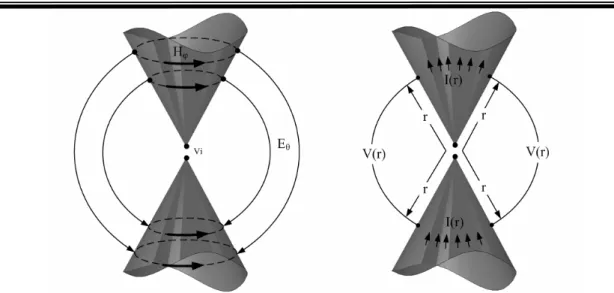
Figure 2.8 Electric and magnetic fields, and associated voltages and currents, for a biconical antenna
For infinite biconical antenna, the magnetic field and electric field can be written as
θ π β φ sin 1 4 0 r e H H r j − = (2-40) θ π η β θ sin 1 4 0 r e H E r j − = (2-41) The far field pattern as θh <θ <π −θh can be written as
θ θ θ sin sin ) ( h F = (2-42) The voltage produced between two corresponding points on the cone, a distance r from
the origin, is written as
⎟ ⎠ ⎞ ⎜ ⎝ ⎛ = − 2 cot ln 2 ) ( 0 j r h e H r V θ π η β (2-43) The current on the antenna, a distance r from the origin, is written as
r j e H r I = −β 2 ) ( 0 (2-44) Using the voltage of (2-43) and current of (2-44), the characteristic impedance as
⎟ ⎠ ⎞ ⎜ ⎝ ⎛ = = 2 cot ln ) ( ) ( 0 h r I r V Z θ π η (2-45) Equation (2-45) indicates that the characteristic impedance is not a function of the radial
CHAPTER 2 BROADBAND ANTENNA BASICS
distance r. The ends of the cone cause reflections that set up standing waves that lead to
a complex input impedance.
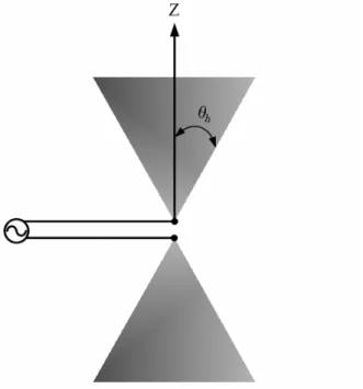
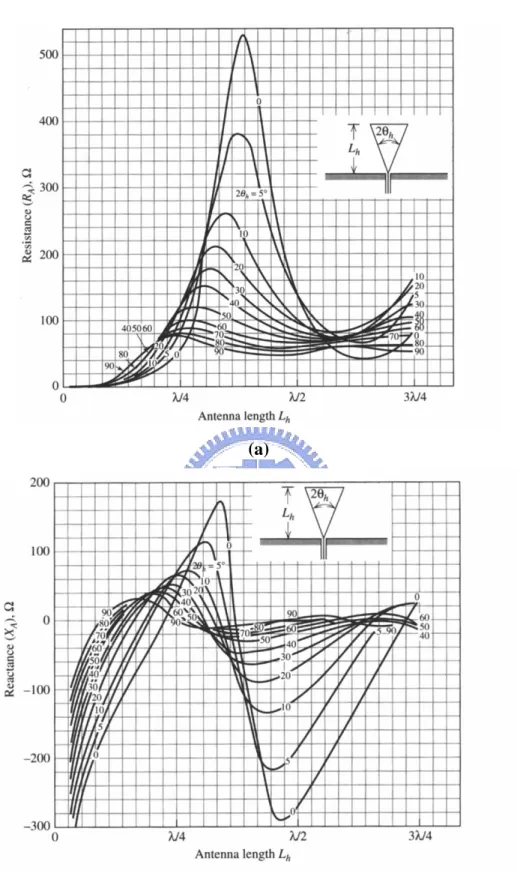
Figure 2.10 indicates that the reactive part of the input impedance can be held to a minimum over a progressively wider bandwidth by increasing the angle θh in Figure 2.9. At the same time, the real part of the input impedance becomes less sensitive to changing frequency.
In Figure 2.10, the impedance of a conical monopole L is plotted versus the h
height of the monopole (L ). This is an example of an antenna that can be more h
dependent on an angle in its geometry description than on its length.
CHAPTER 2 BROADBAND ANTENNA BASICS
(a)
(b)
Figure 2.10 Computed input impedance of a conical monopole with flare angle versus monopole height (a) real part (b) imaginary part.
CHAPTER 3 THE PROPOSED DVB-H ANTENNA
CHAPTER 3 THE PROPOSED DVB-H ANTENNA
In this chapter, section 3.1 presents the design flow of the proposed DVB-H antenna. In Sections 3.2 and 3.3, present the proposed antenna prototype No.1 and prototype No.2, respectively.
3.1 Design Flow of the DVB-H Antenna
It is well known that antenna size, bandwidth, and antenna gain are trade-off with one another. The major challenge in DVB-H antenna design is to provide an internal antenna that is small enough in size whilst maintaining the impedance bandwidth and reasonable antenna gain as required by the specifications.
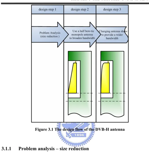
The design purpose of each major step is shown in Figure 3.1. In step one, FR4 with thickness of 0.8 mm is chosen for antenna miniaturization. In step two, the broadband characteristic is created by using a half-bow-tie antenna structure.
CHAPTER 3 THE PROPOSED DVB-H ANTENNA
Figure 3.1 The design flow of the DVB-H antenna
3.1.1
Problem analysis – size reduction
It is well-known that the antenna size is proportional to the wavelength of the operating frequency. Since the quarter-wavelength of DVB-H bands (about10-16 cm) is too large compared with the pocket-size, their antenna sizes need to be reduced to accommodate in a handheld device. Because the wavelength is inversely proportional to the square root of the dielectric constant of the substrate, a substrate with large dielectric constant is suitable for miniaturizing an antenna. It is noted that the radiation efficiency is diminished and have relatively smaller bandwidths [38]. In general the bandwidth is inversely proportional to the square root of the dielectric constant of the substrate [26]. From previous discussion, miniaturized antenna size and bandwidth are trade-off with each other.
CHAPTER 3 THE PROPOSED DVB-H ANTENNA
3.1.2
Broaden the impedance bandwidth
In our design, a bow-tie-like antenna is proposed for broadening the impedance bandwidth. The bow-tie antenna is a planar biconical antenna and is also a broadband antenna. As mentioned in [5], the flare angle of a bow-tie antenna is needed to be greater than 120∘, which yields a large dimension 110×45 mm2 for 470-806 MHz operation and is not suitable for a DVB-H handset. It is well-known that a ground plane may help to reduce the size of a dipole-based antenna. Here, with the help of ground plane surrounding the antenna, a half-bow-tie monopole antenna is proposed. The detail design process is presented in section 3.2.
3.2 Proposed Antenna Prototype No. 1
Figure 3.2 shows the configuration of internal DVB-H antenna prototype No.1. In figure 3.2, the length of the proposed planar monopole is 6 mm5 (about 0.1 wavelength for DVB-H), the width is 18 mm. The gap widths s1, s2, and g are equals to 5mm,
10mm, and 10mm, respectively. It is called as the half-bow-tie monopole antenna that is surrounded by a ground plane. It has small size and suitable shape for a clamshell or a folder-type mobile phone as shown in figure 3.3. In figure 3.3, the clamshell mobile phone is modeled to consist of an upper ground plane and a bottom ground plane. The prototype antenna is mounted on the upper ground plane. The upper and bottom ground planes are connected by a connecting plate.
CHAPTER 3 THE PROPOSED DVB-H ANTENNA
Figure 3.2 The proposed DVB-H antenna prototype No.1
Figure 3.3 Front view of the proposed DVB-H antenna prototype No.1 for a clamshell mobile phone
CHAPTER 3 THE PROPOSED DVB-H ANTENNA
3.2.1
Numerical analysis of antenna prototype No. 1
In the numerical analysis, the size of ground planes and width of the connecting plate are selected the usual dimensions of 90×50 mm2
and 15 mm, respectively, which are similar to commercial clamshell mobile phones.
Figure 3.4 shows simulated return loss versus frequency by varying α. The bandwidth of the antenna is affected by α and it is found α = 9∘yield the largest bandwidth.
The radiation patterns at 500 MHz, 650 MHz, and 780 MHz are shown in Figure 3.5, 3.6, and 3.7 respectively. For the radiation patterns at 500 MHz, 650 MHz, and 780 MHz is near-omnidirectional, which are similar to a monopole.
Figure 3.8 presents the simulated antenna gain over the DVB-H band. The antenna gain varies from 2.5 dBi to 3.6 dBi over the operating band.
CHAPTER 3 THE PROPOSED DVB-H ANTENNA
Figure 3.5 Radiation patterns of DVB-H antenna prototype No.1 at 500 MHz, (a) x-z plane, (b) y-z plane, and (c) x-y plane.
(a) x-z plane (b) y-z plane
CHAPTER 3 THE PROPOSED DVB-H ANTENNA
Figure 3.6 Radiation patterns of DVB-H antenna prototype No.1 at 650 MHz (a) x-z plane, (b) y-z plane, and (c) x-y plane.
(a) x-z plane (b) y-z plane
CHAPTER 3 THE PROPOSED DVB-H ANTENNA
Figure 3.7 Radiation patterns of DVB-H antenna prototype No.1 at 780 MHz (a) x-z plane, (b) y-z plane, and (c) x-y plane.
(a) x-z plane (b) y-z plane
CHAPTER 3 THE PROPOSED DVB-H ANTENNA
CHAPTER 3 THE PROPOSED DVB-H ANTENNA
3.2.2
The Advantages of Antenna Prototype No.1
Compared with [2] – [6] as shown in Table 3.1, our design not only has a simple planar structure but also yields the smallest antenna area and the largest gain with small fluctuation. In [2], [3], and [4], bending a flat metal-plate into U-shaped or L-shaped structure is employed and provides a broadband operation and size reduction. [5] is constructed by a bow-tie structure, the size is 110×45 mm2
which is too large compared with pocket-size.
Table 3.1 Size, bandwidth and gain comparisons between proposed antenna prototype No.1 and other published DVB-H antennas
Antenna area (mm) Size of ground plane (mm2) BW (MHz) /return loss benchmark (dB) Gain (dBi) Proposed Prototype No.1 65×18 180×50, but can be folded to 90×50 500 - 780 / -10 dB 2.5 ~ 3.6 Ref. [2] 75×5×4 (3D structure) 130×75 470 - 702 / -1.25 dB -5 ~ -2.5 Ref. [3] 79×10×5 (3D structure) 300×200 470 - 780 / -7.4 dB 0.8 ~ 1.8 Ref. [4] 65×25×5 (3D structure) 200×78 470 - 850 / -10 dB 1.5 ~ 3.5 Ref. [5] 110×45 300×200 480 - 742 / -7.4 dB 1.5 ~ 2.2 Ref. [6] 90×17 120×80 470 - 810 / -7.4 dB 0.3 ~ 1.7
CHAPTER 3 THE PROPOSED DVB-H ANTENNA
3.3 Proposed Antenna Prototype No.2
In this section, the antenna prototype No. 2 is proposed to improve the bandwidth of the antenna prototype No.1. To broaden No.1’s bandwidth, boundaries, a-b-c, of No.1 antenna are changed and become a curved line as shown in Figure 3.9. The curved line is described by a function: N W x L s y C ⎟ ⎠ ⎞ ⎜ ⎝ ⎛ + = 1 : , 0≤x≤W
where L is the length of the proposed antenna, W is the width of the proposed antenna, and s1 is the gap between antenna and upper ground.
Figure 3.9 The proposed DVB-H antenna prototype No.2. (The curved line C is plotted when N=18.)
3.3.1
Numerical Analysis of Antenna Prototype No.2
Figure 3.10 shows return loss versus frequency of the No.2 antenna with different N. The result clearly indicates that the bandwidth increases with N but the incremental is saturated when N is approaching 18. Therefore, N = 18 is chosen for our design.
CHAPTER 3 THE PROPOSED DVB-H ANTENNA
it is observed that the mutual coupling between the antenna and the upper ground plane may affect the bandwidth. Here, g is changed from 6 mm to 10 mm to find a reasonable bandwidth. It is found that g = 9 mm can provide the largest impedance bandwidth.
Figure 3.12 shows simulated return loss versus frequency by varying tilting angle β. It is noted that the frequency response of our design does not affected by change of the tilting angle. In the figure, the titling angles are in the range of 50º - 60º, which are suitable angles for viewing DTV.
The radiation patterns at 470 MHz, 500 MHz, 550 MHz, 600 MHz, 700 MHz, and 800 MHz are shown in Figure 3.13, 3.14, 3.15, 3.16, 3.17 and 3.18 respectively. From these figures, no special distinctions are observed. The patterns are near-omnidirectional, which are similar to a monopole antenna.
Figure 3.19 presents the simulated antenna gain over the DVB-H band. The antenna gain varies from 2.18 dBi to 3.54 dBi over the operating band.
CHAPTER 3 THE PROPOSED DVB-H ANTENNA
Figure 3.11 Simulated return loss versus frequency by varying gap width (g)
CHAPTER 3 THE PROPOSED DVB-H ANTENNA
Figure 3.13 Radiation patterns of proposed DVB-H antenna at 470 MHz (a) x-z plane, (b) y-z plane, and (c) x-y plane.
(a) x-z plane (b) y-z plane
CHAPTER 3 THE PROPOSED DVB-H ANTENNA
Figure 3.14 Radiation patterns of proposed DVB-H antenna at 500 MHz (a) x-z plane, (b) y-z plane, and (c) x-y plane.
(a) x-z plane (b) y-z plane
CHAPTER 3 THE PROPOSED DVB-H ANTENNA
Figure 3.15 Radiation patterns of proposed DVB-H antenna at 550 MHz (a) x-z plane, (b) y-z plane, and (c) x-y plane.
(a) x-z plane (b) y-z plane
CHAPTER 3 THE PROPOSED DVB-H ANTENNA
Figure 3.16 Radiation patterns of proposed DVB-H antenna at 600 MHz (a) x-z plane, (b) y-z plane, and (c) x-y plane.
(a) x-z plane (b) y-z plane
CHAPTER 3 THE PROPOSED DVB-H ANTENNA
Figure 3.17 Radiation patterns of proposed DVB-H antenna at 700 MHz (a) x-z plane, (b) y-z plane, and (c) x-y plane.
(a) x-z plane (b) y-z plane
CHAPTER 3 THE PROPOSED DVB-H ANTENNA
Figure 3.18 Radiation patterns of proposed DVB-H antenna at 800 MHz (a) x-z plane, (b) y-z plane, and (c) x-y plane.
(a) x-z plane (b) y-z plane
CHAPTER 3 THE PROPOSED DVB-H ANTENNA
Table 3.2 The peak gain and average gain of the proposed antenna prototype No.2
X-Y Plane X-Z Plane Y-Z Plane
peak gain (dBi) average gain(dBi) peak gain (dBi) average gain(dBi) peak gain (dBi) average gain(dBi) 470 MHz 2.10 1.69 1.77 -2.94 2.10 -2.68 500 MHz 2.23 1.76 1.85 -6.30 2.23 -2.92 600 MHz 2.47 1.83 1.99 -3.75 2.48 -3.79 700 MHz 2.77 1.93 2.17 -3.56 2.72 -3.21 800 MHz 3.07 1.92 2.23 -3.17 2.97 -3.05
CHAPTER 3 THE PROPOSED DVB-H ANTENNA
3.3.2
Comparison Between Simulated and Measured Results
According to the proposed antenna of the given dimensions in the last section, the proposed antenna is fabricated by using FR4 substrate. The measured and simulated antenna return losses are compared and shown in Figure 3.20. The return loss is measured by using the Agilent 8719ET Network Analyzer. The figure indicates a good agreement between the measured and simulated results. A wide impedance bandwidth 350MHz (from 450 MHz to 800 MHz) is achieved with return loss less than -10 dB. This result shows that the proposed antenna is suitable for DVB-H receiving antenna in the UHF-band.
The measured radiation patterns at 750 MHz and 800 MHz are shown in Figure 3.21 and Figure 3.22, respectively. The near-omnidirectional patterns are obtained.
CHAPTER 3 THE PROPOSED DVB-H ANTENNA
3.21 Measured Radiation patterns of proposed DVB-H antenna at 750 MHz (a) x-z plane, (b) y-z plane, and (c) x-y plane.
(a) x-z plane (b) y-z plane
CHAPTER 3 THE PROPOSED DVB-H ANTENNA
3.22 Measured radiation patterns of proposed DVB-H antenna at 800 MHz (a) x-z plane, (b) y-z plane, and (c) x-y plane.
(a) x-z plane (b) y-z plane
CHAPTER 3 THE PROPOSED DVB-H ANTENNA
Table 3.3 Size, bandwidth and gain comparisons between our works and other published DVB-H antennas Antenna dimension (mm2) Size of System ground plane (mm2) BW (MHz) / return loss benchmark (dB) Gain (dBi) Proposed Prototype no.1 65×18 180×50, but can be folded to 90×50 500 - 780 / -10 dB 2.5 ~ 3.6 Proposed Prototype No.2 65×18 180×50, but can be folded to 90×50 470 - 800 / -10 dB 2.2 ~ 3.5 Ref [2] 75×5×4 (3D structure) 130×75 470 - 702 / -1.25 dB -5 ~ -2.5 Ref [3] 79×10×5 (3D structure) 300×200 470 - 780 / -7.4 dB 0.8 ~ 1.8 Ref [4] 65×25×5 (3D structure) 200×78 470 - 850 / -10 dB 1.5 ~ 3.5 Ref [5] 110×45 300×200 480 - 742 / -7.4 dB 1.5 ~ 2.2 Ref [6] 90×17 120×80 470 - 810 / -7.4 dB 0.3 ~ 1.7
CHAPTER 4 CONCLUSION
CHAPTER 4 CONCLUSION
In this thesis, a miniaturized DVB-H antenna is constructed by traveling-wave architecture using a bow-tie structure. To achieve DVB-H band, an antenna boundary follows a curve of of x to the power of N function . By dint of x to the power of N, frequency response is realized systematically in the design process. The measurement shows that a wide bandwidth is achieved, about 350 MHz, from 450 MHz to 800 MHz with return loss less than -10dB. The radiation characteristics of the proposed antenna were computed using Ansoft HFSS, which was expected to provide reliable information for the proposed antenna. The computed results shows that the radiation patterns are near-omnidirectional, which are similar to a monopole. The computed antenna gain varies from 2.18 to 3.54 dBi over the DVB-H band and is a reasonable value for DVB-H band.
Reference
References
[1] http://www.fcc.gov/dtv/
[2] J. Holopainen, Antenna for Handheld DVB Terminal, MSc thesis, Helsinki University of Technology, Finland, May 2005.
[3] C.M. Su, L.C. Chou, C.I. Lin, and K.L. Wong, ” Internal DTV receiving antenna for laptop application,” Microwave Opt. Technol. Lett., vol. 44, pp. 4–6, Jan.2005. [4] Y.S. Yu, S.-G. Jeon, H. Park, D.H. Seo, J.H. Choi, “Internal low-profile metal-plate
monopole antenna for DTV portable multimedia player applications,” Microwave
Opt. Technol. Lett., vol. 49, pp. 593-595, Mar.2007.
[5] C.I. Lin, T.Y. Wu, and J.W. Lai, K.L. Wong, “A planar DTV receiving antenna for laptop applications,” Microwave Opt. Technol. Lett., vol. 42, pp. 483–486, Sep.2004.
[6] W.Y. Li,K.L. Wong, and J.S. Row, “Broadband planar shorted monopole antenna for DTV signal reception in a portable media player,” Microwave Opt. Technol.
Lett., vol. 49, pp. 558-561, Mar.2007.
[7] Pey-Ling Teng, Ching-Yuan Chiu, Kin-Lu Wong, “Internal planar monopole antenna for GSM/DCS/PCS folder-type mobile phones,” Microwave Opt. Technol.
Lett., vol. 39, pp. 106-108, Aug.2003
[8] Kin-Lu Wong, Saou-Wen Su, Chia-Lun Tang, and Shih-Huang Yeh, “Internal shorted patch antenna for a UMTS folder-type mobile phone,” IEEE Transactions
on Antennas and Propagation, , Vol. 53, No. 10, October 2005, pp. 3391-, 3394.
[9] Kin-Lu Wong, Wei-Cheng Su, Fa-Shian Chang, “Wideband internal folded planar monopole antenna for UMTS/WiMAX folder-type mobile phone,” Microwave Opt.
Technol. Lett., vol. 48, pp. 324-327, Dec.2005
[10] Bo-Yang Chang, and Jou, C.F, “Compact Antenna Structures for Mobile Handsets,” IEEE 58th Vehicular Technology Conference, 2003 Fall.
[11] M. Martinez-Vázquez, M. Geissler, D. Heberling, A. Martínez-González, D. Sánchez-Hernández, “Compact dual-band antenna for mobile handsets,”
Microwave Opt. Technol. Lett., vol. 32, pp. 87-88, Dec.2001
[12] Dongsheng Qi, Binhong Li, Haitao Liu, “Compact triple-band planar inverted-F antenna for mobile handsets,“ Microwave Opt. Technol. Lett., vol. 41, pp. 483-486, Apr.2004
Reference
broadband antennas,” Helsinki University of Technology, IDC/SMARAD/Radio Laboratory.
[14] J. Ollikainen, O. Kivekäs, A. Toropainen, and P. Vainikainen, “Internal dual-band patch antenna for mobile phones,” Proc. AP2000 Millennium Conference on
Antennas and Propagation, Davos, Switzerland, April 2000, paper p1111.pdf.
[15] Y. –X. Guo, M. Y. W. Chia, and Z. N. Chen, “Miniature built-in multiband antennas for mobile handsets,” IEEE Transactions on Antennas and Propagation, Vol. 52, No. 8, August 2004, pp. 1936-1944.
[16] P. Ciais, R. Staraj, G. Kossiavas, and C. Luxey, “Design of an internal quad-band antenna for mobile phones,” IEEE Microwave and Wireless Components Letters, Vol. 14, No. 4, April 2004, pp. 148-150.
[17] S. Yong-Sun, K. Byoung-Nam, K. Won-Il, and P. Seong-Ook, “GSM/DCS/IMT-2000 triple-band built-in antenna for wireless terminals,” IEEE
Antennas and Wireless Propagation Letters, Vol. 3, 2004, pp. 104 – 107.
[18] M. Martinez-Vázques, and O. Litschke, “Quadband antenna for handheld personal communications devices,” IEEE Antennas and Propagation Society International
Symposium, Vol. 1, Ohio, USA, June 2003, pp. 455 – 458.
[19] P. –L. Teng, H. –T. Chen, and K. –L. Wong, “Multi-frequency planar monopole antenna for GSM/DCS/PCS/WLAN operation,” Microwave and Optical
Technology Letters, Vol. 36, No. 5, March 2003, pp. 350 – 352.
[20] Q. –Y. Lee, and K. –L. Wong, “Quad-band internal monopole mobile phone antenna,” Microwave and Optical Technology Letters, Vol. 40, No. 5, March 2004, pp. 359 – 361.
[21] P. Vainikainen, J. Ollikainen, O. Kivekäs and I. Kelander, ”Resonator-based analysis of the combination of mobile handset antenna and chassis,” IEEE
Transactions on Antennas and Propagation, Vol. 50, No. 10, October 2002, pp.
1433-1444.
[22] Nader Behdad, and Kamal Sarabandi, “A compact antenna for ultrawide-band applications,” IEEE Transactions on Antennas and Propagation, Vol. 53, No. 7, July 2005, pp. 2185-2192.
[23] Jianming Qiu, Zhengwei Du, Jianhua Lu, and Ke Gong, “A Planar Monopole Antenna Design With Band-Notched Characteristic,” IEEE Transactions on
Antennas and Propagation, Vol. 54, No. 1, January 2006, pp. 288-292.
[24] A. M. Abbosh, M. E. Bialkowski, J. Mazierska, and M. V. Jacob, “A planar UWB antenna with signal rejection capability in the 4-6 GHz Band,” IEEE
MICROWAVE AND WIRELESS COMPONENTS LETTERS, VOL. 16, NO. 5, pp.
Reference
[25] A. Burtrym, and S.Pivnenko, “CPW to CPS Transition for Feeding UWB Antennas,” IEEE A&E Systems Magazine, pp. 21-23, Feb. 2006.
[26]Constantine A. Balanis, Antenna Theory: Analysis and Design 3rd ed, John Wiley & Sons Inc, 2005.
[27] Warren L. Stutzman and Gary A. Thiele, Antenna Theory and Design, 2nd ed., John Wiley & Sons, Inc., 1998.
[28]David M. Pozar, Microwave Engineering, 3rd ed., John Wiley & Sons, Inc., 2005. [29] K. L.Wong, C. L. Tang, and H. T. Chen, “A compact meandered circular
microstrip antenna with a shorting pin,” Microwave Opt. Technol. Lett. 15, 147–149, June 20, 1997.
[30] 吳武順﹐以碎形特徵作玻璃上數位電視平面天線之設計﹐私立大同大學通訊 工程研究所碩士論文﹐中華民國九十四年十月。