行動無線感測網路下基於能源節約的叢集式路由方法

國

立

交

通

大

學

資訊科學與工程研究所

碩

士

論

文

行動無線感測網路下基於能源節約的

叢集式路由方法

A Cluster-Based Energy Efficient Routing Algorithm in Mobile

Wireless Sensor Networks

研 究 生：張泰榕

指導教授：王國禎 教授

行動無線感測網路下基於能源節約的叢集式路由方法

A Cluster-Based Energy Efficient Routing Algorithm in Mobile

Wireless Sensor Networks

研 究 生：張泰榕 Student：Tai-Jung Chang

指導教授：王國禎 Advisor：Kuochen Wang

國 立 交 通 大 學

資 訊 科 學 與 工 程 研 究 所

碩 士 論 文

Submitted to Department of Computer Science and Engineering College of Computer Science

National Chiao Tung University in Partial Fulfillment of the Requirements

for the Degree of Master

in

Computer Science June 2006

Hsinchu, Taiwan, Republic of China

中華民國九十五年六月

行動無線網路下基於能源節約的叢集式路由方法

學生：張泰榕 指導教授：王國禎 博士

國立交通大學資訊學院 資訊科學與工程研究所 碩士班

摘 要

散佈在無線感測網路下的各個節點對於周圍環境有感測、計算與傳

送的能力。由於GPS的價格昂貴，我們使用少部分不會移動的錨節點(已

知位置)來幫助我們計算其他的感測節點的位置。為了有效率地傳送感

測資料到目的地(伺服器)，確認每個感測節點的位置對於建置路由有

很大的幫助。我們使用一個基於色彩理論的行動定位演算法，CDL [1]，

來幫助感測節點的定位。因為感測節點的能源是有限的，我們提出一

個基於能源節約的叢集式路由方法(CEER)來延長感測節點的使用壽

命。CEER把整個目標區域分割成許多個子區域(網格)，使得每個在網

格內的感測節點彼此都能在無線電範圍內，然後每個網格都會選出一

個叢集頭。每個錨節點會廣播自己的RGB值及位置資訊到各個感測節

點，包括叢集頭。每個感測節點會週期性的把感測資料(如果有的話)

及其RGB值資訊傳送到對應的叢集頭。接下來叢集頭會把聚集的資料利

用兩個步驟經由錨節點傳送到伺服器。步驟一是它會比較叢集成員中

的RGB值以選擇一些更接近所屬錨節點的感測節點當作下一個可能的

跳躍點。步驟二是叢集頭會在那些被選中的叢集成員中找尋具最大能

源的感測節點當作下一個跳躍點。本方法的獨特性在於藉由比較鄰近

節點對應的RGB值資訊，可以找到一條考量到能源的路由。模擬的結果

顯示，與另一個在行動無線感測網路下的路由方法ESDSR[2]相比，CEER

的平均能源節約比ESDSR好約 50-60%。另外，CEER的平均封包傳送時間

比ESDSR少約 50%。

關鍵詞：基於色彩理論的動態定位技術，叢集，行動無線感測網路，

路由方法。

A Cluster-based Energy Efficient Routing

Algorithm in Wireless Sensor Networks

Student：Tai-Jung Chang Advisor：Dr. Kuochen Wang

Department of Computer Science and Engineering National Chiao Tung University

Abstract

Wireless sensor networks (WSNs) with nodes spreading in a target area have abilities of sensing, computing, and communication. Since the GPS device is expensive, we use a small number of fixed anchor nodes that are aware of their locations to help estimate the locations of other sensor nodes in WSNs. To efficiently route sensed data to the destination (the server), identifying the location of each sensor node can be of great help. We adopted a range-free Color-theory based Dynamic Localization, CDL [1], to help identify each sensor node’s location. Since sensor nodes are battery-powered, we propose a Cluster-based Energy Efficient Routing algorithm (CEER) to prolong the life time of each sensor node. CEER divides a target area into sub-areas called grids such that all sensor nodes in a grid are within the radio range, and a cluster head is selected in each grid. Each anchor will broadcast its RGB values to each sensor node, including cluster heads. A sensor node will periodically forward its RGB values along with sensed data (if available) to its associated cluster head. The cluster head will then forward the aggregated data to a nearby anchor in two steps. In step 1, it selects those cluster members that are closer to the anchor than itself as next possible hops by comparing their RGB values. In step 2, among those selected cluster members, the sensor node with the highest energy level is selected as the next hop. The uniqueness of our approach is that by comparing the associated RGB values among neighboring nodes, we

can efficiently choose a better routing path with energy awareness. Simulation results have shown that our routing algorithm can save 50% - 60% energy than ESDSR [2] in mobile wireless sensor networks. In addition, the latency per packet of CEER is 50% less than that of ESDSR.

Keywords: CDL, cluster-based, localization, mobile wireless sensor network, routing

algorithm.

Acknowledgements

Many people have helped me with this thesis. I deeply appreciate my thesis advisor, Dr. Kuochen Wang, for his intensive advice and instruction. I would like to thank all the classmates in Mobile Computing and Broadband Networking Laboratory for their invaluable assistance and suggestions. The support by the National Science Council under Grant NSC94-2213-E-009-043 is also grateful acknowledged.

Finally, I thank my Father and Mother for their endless love and support.

Contents

Abstract (in Chinese) i

Abstract (in English) iii

Acknowledgements v Content vi List of Figures viii List of Tables ix Chapter 1 Introduction……… 1

Chapter 2 Preliminary of CDL……… 3

2.1 The Information Delivery of Anchors [1]……… 3

2.2 The Establishment of Location Database [1]……… 4

2.3 Mobility [1]……… 5

Chapter 3 Related Work……… 6

3.1 Existing Routing Protocols……… 6

3.1.1 Flat routing – Sensor Protocols for Information via Negotiation (SPIN) [4]……… 6

3.1.2 Hierarchical routing – Two Tier Data Dissemination (TTDD) [5]……… 7

3.1.3 Location based routing – Geographic and Energy Aware Routing (GEAR) [6]……… 8

3.1.4 Source routing – Dynamic Source Routing (DSR) [7] and Energy Saving DSR (ESDSR) [2]……… 9

3.2 Comparison of Different Routing Protocols……… 10

Chapter 4 Cluster-based Energy Efficient Routing Algorithm…… 12

4.1 Network Model……… 12

4.2 Setup Phase……… 12

4.3 Data Dissemination Phase……… 14

4.4 Refinement Phase……… 15

Chapter 5 Simulation Results and Discussion……… 18

5.1 Simulation Model……… 18

5.2 Comparison with ESDSR [2] ……… 19

Chapter 6 Conclusion and Future Work……… 22

6.1 Concluding Remarks……… 22

6.2 Future Work……… 22

Bibliography 24

List of Figures

Figure 1 Flat routing – SPIN……… 7

Figure 2 Hierarchical routing – TTDD……… 8

Figure 3 Location based routing – GEAR……… 9

Figure 4 Setup phase 1……… 13

Figure 5 Setup phase 2……… 13

Figure 6 Data dissemination step 1……… 14

Figure 7 Data dissemination step 2……… 15

Figure 8 The flowchart of CEER……… 17

Figure 9 Anchor deployment……… 19

Figure 10 Energy consumption vs. number of nodes……… 20

Figure 11 Latency per packet vs. number of nodes……… 20

Figure 12 Number of dead nodes at the end of simulation……… 21

List of Tables

Table 1 Comparison of six routing protocols……… 11

Table 2 Simulation parameters……… 19

Chapter 1

Introduction

With the recent technology, small and low-cost sensors have become feasible in our daily life. These sensor nodes sense data in the environment surrounding them and transmit the sensed data to the sink (or the server). The way to transmit sensed data to the server affects the power usage of each node deeply. Typically, wireless sensor networks (WSNs) contain hundreds or thousands of sensor nodes and these sensor nodes have the ability to communicate with either among each other or directly to the destination (sink). Using a larger number of sensor nodes allows for sensing over wider geographical regions with greater accuracy. Sensor nodes may use up their energy so that they probably become unavailable in the WSNs during communications or measurements. With more and more sensor nodes become unavailable, a WSN may be separated into several sub-networks or become sparse. It is not desirable for a WSN to be separated to several sub-networks or become sparse because communications and measurements becomes difficult and less accuracy.

It is a great challenge for routing in WSNs due to the following reasons. First, since it is not easy to build a whole network topology, it is hard to assign each routing path. Secondly, sensor nodes are tightly constrained in terms of energy, processing, and storage capacities. Thus, they require effective resource management policies, especially efficient energy management, to increase the lifetime of a WSN.

The proposed routing algorithm is based on a range-free color-theory-based dynamic localization algorithm, CDL [1], in which the location of a sensor node is represented as a set of RGB values. With known RGB values for each sensor node, we

-can find out the most possible position of a node by looking up the location database in the server. To keep track of a sensor node’s location, frequently updating the RGB values of each sensor node and delivering the update to the server is necessary. However, if battery-powered nodes frequently update their positions, they may consume energy quickly and also waste bandwidth.

The CEER selects those cluster members that are closer to the anchor than itself as next possible hops by comparing their RGB values. Among those selected cluster members, the sensor node with the highest energy level is selected as the next hop.

The remainder of this thesis is organized as follows. Chapter 2 briefly introduces the CDL algorithm that is the basis of our routing algorithm. Chapter 3 introduces five related approaches and explains how they work. The network model and the proposed cluster-based energy efficient routing algorithm are described in Chapter 4 in detail. Chapter 5 evaluates and compares our approach with some classical approaches. Simulation results demonstrate the merits of our cluster-based energy efficient routing algorithm. Finally, concluding remarks and future work are given in Chapter 6.

-Chapter 2

Preliminary of CDL

In this chapter, we introduce the color-theory-based dynamic localization, the CDL algorithm [1]. This centralized localization algorithm is based on the color theory to perform positioning in mobile wireless sensor networks. It builds a location database in the server, which maps a set of RGB values to a geographic position. And the distance measurements by sensor nodes are based on the DV-Hop [3]. When a sensor node receives anchors’ RGB values, it calculates its own RGB values. The node then sends its RGB values to the server so that the server can find the most possible location by looking up the location database.

2.1 The Information Delivery of Anchors [1]

In this section, we introduce some notations that are defined in CDL:

¾ Each node i maintains an entry of and , where k represents the

k ) , , (R_ik G_ik B_ik D_ik th anchor.

¾ D_avg is the average hop distance, which is based on DV-Hop [3]. ¾ h_ij is the hop distance between nodes i and j.

¾ D_ik represents the hop distance from anchor k to node i : D_ik =D_avg ×h_ik

¾ Range represents the maximum distance that a color can propagate. ¾ (R_k,G_k,B_k) is the RGB value of anchor k.

¾ (H_ik,S_ik,V_ik) is the HSV values of anchor k received by the ith node.

The RGB values of anchors are assigned randomly from 0 to 1. After a sensor node i

-obtains each anchor k’s RGB values and hop distance ( ), the RGB values are first converted to HSV values by equation

ik h (1): ) , , (H_k S_k V_k = RGBtoHSV(R_k,G_k,B_k) (1)

With , can be computed. The updated HSV values corresponding to node i of

anchor k are calculated by equation ik h D_ik (2). k ik H H = , S_ik =S_k, _ik ik V_k Range D V =(1− )× (2) The RGB values of node i corresponding to anchor k are then calculated:

) , ,

(R_ik G_ik B_ik = HSVtoRGB (H_ik,S_ik,V_ik) (3) The RGB values of node i are the mean of the RGB values corresponding to all anchors, and are computed as follows:

∑

where n is the number of anchors that node i received.

2.2 The Establishment of Location Database [1]

A location database is established when the server obtains the RGB values and locations of all anchors. The mechanism is based on the theorem of the mixture of different colors. With the RGB values of all anchors, the RGB values of all locations can be computed by exploiting the ideas of color propagation and the mixture of different colors. In the first place, the distance between each location i and anchor k is obtained:

ik

d =

(

x

−

x

)

+

(

y

−

y

)

where is the coordinate of location i, and is the location of anchor k.

First of all, we have to calculate the HSV values of each location i corresponding to anchor k:

) ,

(xi yi

(

x

,

y

)

-) , , (H_k S_k V_k = RGBtoHSV(R_k,G_k,B_k) (6) k ik H H = , S_ik =S_k , _ik ik V_k Range d V =(1− )• (7) The RGB values of location i corresponding to anchor k can be derived by equation (8):

) , ,

(R_ik G_ik B_ik = HSVtoRGB(H_ik,S_ik,V_ik) (8) Then the RGB values of location i can be calculated by averaging all RGB values of location i corresponding to N anchors.

∑

where N is the number of anchors.

In this way, the location for each sensor node can be constructed in the location

database by maintaining the coordinate and the RGB value at

each location i. Then, the location of a sensor node can be acquired by looking up the location database based on the derived RGB values.

) ,

(x_i y_i (R_i,G_i,B_i)

2.3 Mobility [1]

When a mobile node arrives at a new location, it sends an anchor information request to neighbor nodes. If a neighbor node has the anchors’ RGB values, it transmits packets that include the RGB values of each anchor and the hop count from the anchor to the node. After receiving the packets from neighbors, node i compares and calculates the D_ik to the kth anchor and gets the smallest . With the RGB values and to all anchors, node i can update its RGB values using equation

ik

D D_ik

(1), (2), (3), and (4). The new RGB values are then transmitted to the server and the position of node i will be updated by looking up the location database.

-Chapter 3

Related Work

3.1 Existing Routing Protocols

In this chapter, we introduce several routing protocols in WSNs, which can be categorized into flat routing, hierarchical routing, location based routing, and source

routing. Flat routing is that when a node queries for data in its communication range,

neighbor nodes which have data will transmit the data to that node which is data-centric routing, such as SPIN [4] and Direct Diffusion [11]. Hierarchical routing builds a hierarchical topology in the region. It performs data aggregation and fusion in cluster heads in order to decrease the number of transmitted messages to the base station, such as TTDD [5], LEACH [12], and PEGASIS [13]. As to the location based routing, sensor nodes are addressed by means of their locations. We can use the direction of the destination to forward data to the nearest neighborhood recursively until reaching the destination, such as GEAR [6] and SPAN [14]. Source routing is a routing technique in which the source node determines the complete sequence of nodes to forward the packet; the source node explicitly lists this route in the packet’s header, identifying each forwarding “hop” by the address or node’s ID of the next node to transmit the packet on its way to the destination node, such as DSR [7], AODV [15], and SPEED [16]. In the following, we review a classical routing protocol in each category.

3.1.1 Flat routing – Sensor Protocols for Information via Negotiation (SPIN) [4]

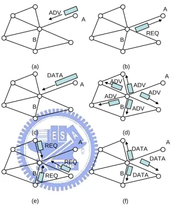
SPIN, also known as Sensor Protocols for Information via Negotiation, disseminates all the information at each node to neighbor nodes in the network. A source node first advertises its data to neighbor nodes. If a node within the radio range wants the data advertised by the source node, it sends a reply packet to the source node.

-The source node will send data to the request node which queried for the data. This is illustrated in Figure 1. The disadvantage of SPIN is that it can’t guarantee the delivery

of interested data. If a node is interested in the data that is far away from the source node and nodes between source and destination nodes are not interested in that data, data will not be delivered to the destination node at all.

B B REQ B A B A DATA ADV ADV ADV ADV ADV B A B A DATA DATA DATA REQ REQ REQ (a) (b) (c) (d) (e) (f) A ADV A

Figure 1. Flat routing – SPIN. Node A starts by advertising its data to node B (a). Node B responds by sending a request to node A (b). After receiving the requested data (c), node B then sends out advertisements to its neighbors (d), who in turn send requests back to B (e,f) [4]

3.1.2 Hierarchical routing – Two Tier Data Dissemination (TTDD) [5]

An approach that provides data delivery to multiple mobile sinks is called TTDD, is illustrated in Figure 2, which is two tier data dissemination. Each data source proactively builds a grid structure that is used to disseminate data to the mobile sinks by assuming that sensor nodes are stationary and location aware. The sink chosen by the server may leave its old position to another position. Once this occurs, sensor nodes

-surrounding the sink process the signal sent by the sink and one of them becomes the new source node to generate data reports.

B

S

Node Source Sink

Figure 2. Hierarchical routing – TTDD. One source B and one sink S [5]

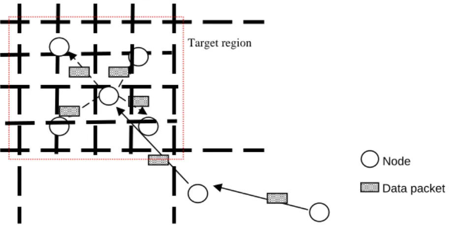
3.1.3 Location based routing – Geographic and energy aware routing (GEAR)

This algorithm, as illustrated in Figure 3, discusses the use of geographic inform

[6]

ation while disseminating queries to appropriate regions since data queries often include geographic attributes. Each node in GEAR keeps an estimated cost and a learning cost of reaching the destination through its neighbors. The estimated cost is a combination of residual energy and distance to the destination. The learning cost is refinement of the estimate cost that accounts for routing around holes in the network. A hole occurs when a node does not have any closer neighbor to the target region than itself. Two phases are used in this algorithm, forwarding packets towards the target region and forwarding packets within the region. In the first phase, when receiving a packet, a node checks its neighbors to see if one neighbor node is closer to the target region than itself. In the second phase, if the packet reaches the target region, it can be

-diffused in that region by using recursive geographic forwarding or restricted flooding.

Node Data packet

re 3. Location based routing – GEAR. Recursive geogra

Target region

Figu ic forwarding: data disseminate to four

SR) [7] and ESDSR [2]

he to store

aintenance operation is the mechanism which a node is able to detect any

ph sub-regions recursively until regions with only one node are left [6]. 3.1.4 Source Routing – Dynamic Source Routing (D

The DSR routing [7] is based on the source routing. It uses each node’s cac information about the routing path which will be maintained by each sensor node if the routing path is broken or not. Two operations are used to build a routing path,

route discovery and routing maintenance. Route discovery is the mechanism by which a

source node finds a route to the destination. When a source wants to send information to the destination, it searches its own cache to find a routing path. If the source node can not find a routing path to the destination, it starts to perform route discovery. First of all, the source node initiates a local broadcast to start the routing. If the node which receives the packet is the route destination, it will route back to the source node. If it is not the destination, it also broadcasts a packet to its neighbors until reaching the destination. The source will choose the shortest path — the smallest hop count path — to route to the destination.

The route m

changes in the network topology. While a node is unavailable, its one hop neighbor nodes around the routing path should route back to the source such that every node’s caches can update the new information.

-ESDSR [2] is an energy efficient DSR protocol. It changes the way of choosing a routi

g Protocols

A ty, position awareness, and loca

ng path from the shortest path in DSR to the maximum expected life of the path. Once a source node setups a route discovery, the return packet of each route path will contain the minimum expected battery life. The source node chooses a routing path with the maximum expected battery life among all routing paths. Each node also has its power table which contains its neighbor’s power state information so that it will choose more energy efficient path to the destination.

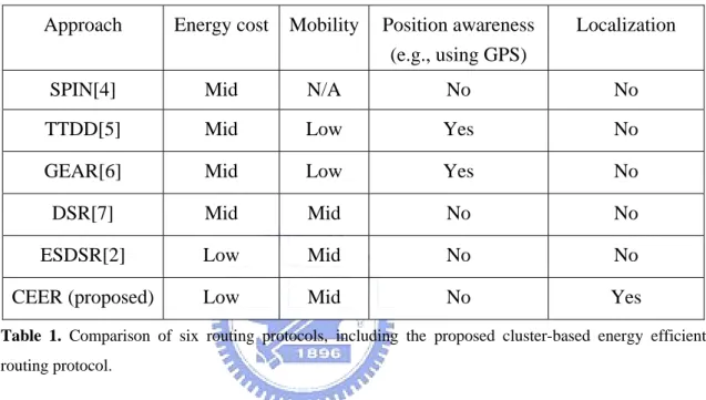
3.2 Comparison of Different Routin

ccording to the following metrics: energy cost, mobili

lization, the above mentioned approaches are compared, as shown in Table 1. The

proposed cluster-based energy efficient routing (CEER) is also included in the table, which will be described in Chapter 4. First, the metric of energy cost indicates the average energy cost of the protocol for a packet sending from the source to the destination. ESDSR, which is the energy saving version of DSR will be evaluated in our simulations later. Mobility indicates whether nodes in the WSN are fixed or mobile. DSR, ESDSR, and the proposed CEER can support mobility. The position awareness indicates that if a protocol needs each node to know its position, e.g., using GPS. TTDD and GEAR require this information to route data to the destination. The last metric, localization, indicates that the proposed CEER can perform localization because the source node uses RGB values to assist routing.

-Approach Energy cost Mobility Position awareness (e.g., using GPS)

Localization

SPIN[4] Mid N/A No No

TTDD[5] Mid Low Yes No

GEAR[6] Mid Low Yes No

DSR[7] Mid Mid No No

ESDSR[2] Low Mid No No

CEER (proposed) Low Mid No Yes

Table 1. Comparison of six routing protocols, including the proposed cluster-based energy efficient

routing protocol.

-Chapter 4

Cluster-based Energy Efficient

Routing Algorithm

In this chapter, we propose a cluster based energy efficient routing (CEER) algorithm for WSNs, which is based on the CDL [1]. The network model is first described. The routing process can be organized into three phases: setup phase, data dissemination phase, and refinement phase, which will be described next.

4.1 Network Model

The network model for our routing protocol is described as follows:

¾ A server is used for building a location database, localization, and collecting sensed data.

¾ The area is divided into clusters and a cluster head is selected by the server for each cluster.

¾ There are four anchors, which are placed in the four corners of the area [9]. Anchors collect aggregate data received from cluster heads.

¾ All sensor nodes have a uniform energy at the beginning.

¾ Each node wakes up at a fixed rate to check if its RGB values have changed. ¾ All sensor nodes are mobile.

¾ CSMA/CA is used to avoid collision of packets.

4.2 Setup Phase

In this phase, we need to choose a sensor node to be the cluster heads so that we can start to collect data. First, we used a sensor node’s radio range R such that the grid size is R× . All sensor nodes in a cluster (grid) are within their cluster head’s radio R

-range.

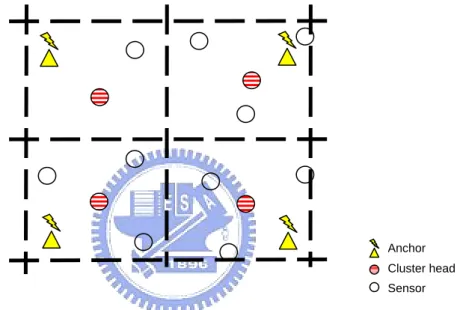
Secondly, each anchor floods its RGB values and average hop distance to each sensor node so that it can calculate its hop count to the anchor and adjust its RGB values based on the hop count. Then, the server receives the RGB values from each sensor node. By looking up the location database, the server can calculate each sensor node’s location and choose a cluster head which is close to the center of the grid, as shown in Figure 4.

Anchor Cluster head Sensor

Figure 4. Setup phase 1: Choose a cluster head which is close to the center of the grid.

Finally, the server uses the closest anchors to send information to the selected sensor nodes to let them know that they are cluster heads, as shown in Figure 5.

Anchor Cluster head

Figure 5. Setup phase 2: Server uses the closest anchors to send information to the selected sensor nodes to let them know that they are cluster heads.

-4.3 Data Dissemination Phase

After the setup phase, each cluster head will receive its cluster member’s information. If a sensor node’s position is changed, its hop counts to the anchors may also change. The node then updates its RGB values and transmits them to its cluster head. When a cluster head receives information from its cluster member, it will setup a timer and wait for other possible information from other members until the timer expires. The advantage of setting up a timer is that we can wait for other cluster members to see if they have data to send. In this way, communication cost can be reduce.

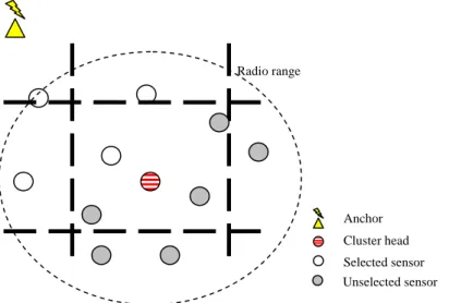
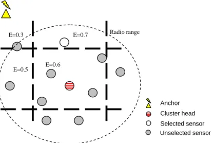
When a cluster head wants to forward the aggregate data toward the server, two steps are performed in CEER. In the first step, it selects its one hop neighbors that are closer to a nearby anchor than itself as the next possible hop by comparing their respective RGB values, as shown in Figure 6. In the second step, among those selected cluster members, the sensor node with the highest energy level is selected as the next hop, as shown in Figure 7. The selected node will receive the aggregated data and again follows these two steps to transmit the data to its next hop until reaching the server via the anchor. Radio range Anchor Cluster head Selected sensor Unselected sensor

Figure 6. Data dissemination step 1. Select one hop neighbor nodes closer to the anchor

-E=0.6 E=0.7 E=0.3 E=0.5 Radio range Anchor Cluster head Selected sensor Unselected sensor

Figure 7. Data dissemination step 2. Choose the node with the maximum energy level from the selected nodes

4.4 Refinement Phase

There are several situations that a cluster head may fail to do its job. For example, if a cluster head has low power, it may not live long enough to be a cluster head. On the other hand, if a cluster head moves away from the grid, it may lose contact with some cluster members. In these situations, it is necessary to choose another sensor node to become a new cluster head so that the information can still be forwarded.

However, if we change cluster heads too often, it will waste too much energy and communication cost to switch the cluster head’s job from one sensor node to another. Our approach uses the server to choose cluster heads because the server knows the speed, position, and energy level of each node. Among them, the most important factor is a node’s energy level. However, under the following two conditions, the role of a cluster head will not be replaced:

¾ A cluster head with an energy level higher than half of the original battery capacity.

¾ A cluster head with an energy level lower than half of the original battery capacity but higher than the average energy level.

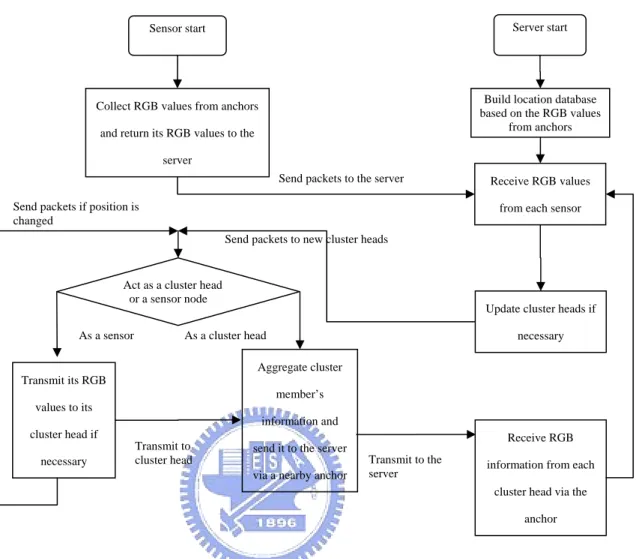
-If a cluster head with low energy needs to be replaced, the server collects information of the sensor nodes in the corresponding grid. Then the server sorts each node’s speed from low to high and chooses a node if its energy level is higher than half of the original battery capacity or higher than the average energy level. On the other hand, when a sensor moves away from its cluster head, it broadcasts a packet to its neighbor nodes to ask for a new cluster head and hop counts. If there are more than two cluster heads for the sensor node to choose, the cluster head with RGB values closer to itself will be chosen. Figure 8 is the flowchart of our CEER algorithm.

-Sensor start

Collect RGB values from anchors and return its RGB values to the

server

Server start

Build location database based on the RGB values

from anchors

Receive RGB values from each sensor

Update cluster heads if necessary Transmit its RGB values to its cluster head if necessary Aggregate cluster member’s information and send it to the server via a nearby anchor As a sensor As a cluster head

Receive RGB information from each

cluster head via the anchor Act as a cluster head

or a sensor node

Send packets to new cluster heads

Transmit to

cluster head Transmit to the server Send packets if position is

changed

Send packets to the server

Figure 8. The flowchart of CEER

-Chapter 5

Simulation Results and Discussion

In this chapter, we evaluate the proposed approach, CEER, by measuring its energy consumption and latency per packet with different number of sensor nodes and compare it with an existing approach, ESDSR [2].

5.1 Simulation Model

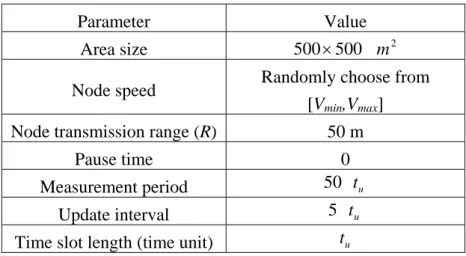
Our simulation model follows that of CDL [1] since our routing algorithm is based on CDL. All nodes were randomly placed in a 500 m × 500 m area and a modified random waypoint models [8] was used to simulate the mobility characteristic of each sensor node. In addition, a sensor node selects a moving destination and a velocity randomly. After reaching the destination, the sensor node pauses for a period of time (pause time). The node speed is uniformly distributed within [Vmin, Vmax]. The

simulation parameters are shown in Table 2. The two performance parameters are defined as follows:

¾ Total energy consumption (mJ): summary of all sensor nodes’ energy consumption after 50 time slots (time units).

¾ Latency per packet (sec): average time spent to send a packet with aggregate data such as RGB values from a sensor node to the server.

-Parameter Value

Area size 500×500 m2

Node speed Randomly choose from

[Vmin,Vmax]

Node transmission range (R) 50 m

Pause time 0

Measurement period 50 tu

Update interval 5 tu

Time slot length (time unit) t u

Table 2. Simulation parameters.

In [9], it has shown that the location estimated error is minimized when anchors are placed at the corners. So we put four anchors at the four corner of the area, as shown in Figure 9.

Anchor

Figure 9. Anchor deployment.

5.2 Comparison with ESDSR [2]

Sooyeon Kim et. al [10] mentioned that a well dissemination routing protocol should have three characteristics: energy efficient, self-configuration, and scalable. By simulations, we have shown that our algorithm is better than ESDSR in terms of energy efficiency. Our algorithm is self-configurable in terms of cluster head selection, as described section 4.4. As to the scalability, our algorithm is more scalable than ESDSR when the area is bigger, which will be described at the end of this section.

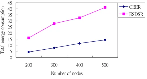
-0 5 10 15 20 25 30 35 40 45 200 300 400 500 Number of nodes

Total energy consumption

CEER ESDSR

Figure 10. Energy consumption vs. number of nodes

As shown in Figure 10, our approach (CEER) saves more energy than ESDSR when the number of nodes increases. This is because CEER uses a cluster head to aggregate data and adopts dynamic path finding to find a neighbor node with maximum energy to route data to a nearby anchor. ESDSR uses local broadcast to find a path and choose the best route with maximum expected life but the source node doesn’t aggregate data of its neighbor nodes to send data to the destination.

0 1 2 3 4 5 200 300 400 500 Number of nodes

Latency per packet(sec)

CEER ESDSR

Figure 11. Latency per packet vs. number of nodes.

In Figure 11, CEER has less latency per packet than ESDSR because the ESDSR uses the path with the maximum expected life in order to balance the load of the entire

-sensor network. In contrast, our approach selects a next hop node to delivery data based on the RGB values and the maximum energy levels of neighbor nodes, which is more efficient.

We also used the same network model as that of ESDSR [2] to validate the correct implementation of the ESDSR and CEER. Forty sensor nodes were randomly placed in an area sized from 200 m × 200 m, 300 m × 300 m, 400 m × 400 m, to 500 m × 500

m, respectively, while keeping the number of mobile nodes (40) and connection (20)

constants. Figure 12 shows that, in a small area, our approach did not perform well compared to ESDSR. This is because we used a cluster head to forward transmissions, even if a node is within the transmission range of an anchor. When the area grows bigger, the routing path is long enough so that the overhead of routing packets to the cluster head can be reduced. Therefore, CEER is more scalable than ESDSR when the area is growing bigger.

0 2 4 6 8 10 12 40 90 160 250 Area (1000 ) Numbe r of dead nodes CEER ESDSR

Figure 12. Number of dead nodes at the end of simulation 2

m

-Chapter 6

Conclusion and Future Work

6.1 Concluding Remarks

In this paper, we have presented a cluster-based energy efficient routing algorithm (CEER) based on a color-theory-based dynamic localization algorithm (CDL). The basic idea of CEER is based on comparing the RGB values of neighbor nodes and those neighbor nodes that are closer to a nearby anchor are selected. Among these selected neighbor nodes, a sensor node with the highest energy level is chosen to be the next hop node toward the server via the anchor. Simulation results have shown that our routing algorithm can save 50% - 60% energy compared to ESDSR [2] in mobile wireless sensor networks. In addition, the latency per packet of CEER is 50% less than that of ESDSR.

6.2 Future Work

We will focus on how to set an appropriate updating interval of the RGB values of sensor nodes. Note that cluster heads are assigned by the server. If the update interval is too long, a cluster head may leave its associated cluster. This situation leads to no cluster head in the cluster. If the update interval is too short, it wastes energy and bandwidth. Therefore, the problem of determining a suitable update interval deserves to further study. In addition, applying our routing algorithm to a real system, such as a community health care system, will be our further work as well.

-Bibliography

[1] Shen-Hai Shee, Kuochen Wang, and I.L. Hsieh “Color-theory-based Dynamic Localization in Mobile Wireless Sensor Networks,” in Proceedings of Workshop on

Wireless, Ad Hoc, Sensor Networks, Aug. 2005.

[2] Mohammed Tarique, Kemal E. Tepe, and Mohammad Naserian, ”Energy Saving Dynamic Source Routing for Ad Hoc Wireless Networks,” in Proceedings of

Modeling and Optimization in Mobile, Ad Hoc, and Wireless Networks, pp. 305-310.

April 2005

[3] J.G. Lin and S.V. Rao, “Mobility-enhanced Positioning in Ad Hoc Networks, ”

IEEE Wireless Communications and Networks Conference, vol.3, pp. 1832-1837,

Mar. 2003

[4] W. Heinzelman, J. Kulic and H. Balakrishnan, ”Adaptive Protocols for Information

Dissemination in Wireless Sensor Networks,” in Proc. 5th ACM/IEEE mobicom,

Seattle, WA, pp. 174-85, Aug. 1999.

[5] F. Ye et al., “A Two-Tier Data Dissemination Model for Large-Scale Wireless Sensor Networks,” in Proc. ACM/IEEE MOBICOM, pp. 148-159, 2002

[6] Y.Yu, D. Estrin, and R.Govindan, “Geographical and Energy-Aware Routing: A Recursive Data Dissemination Protocol for Wireless Sensor Networks,” UCLA

Comp. Sci. Dept. Tech. Rep.,UCLA-CSD TR-010023, May 2001.

[7] J. Borch, D. B. Johnson, and D. A. Maltz, “The Dynamic Source Routing Protocol for Mobile Ad Hoc Networks”, IETF Internet_Draft, draft-ietf-manet-dsr-00.txt, March 1998.

[8] J. Yoon, M. Liu, B. Noble, “Random waypoint considered harmful,”.

Twenty-Second Annual Joint Conference of the IEEE Computer and Communications Societies. IEEE INFOCOM. pp. 1312-1321. April 2003.

[9] Hongyi Wu, Chong Wang, and Nian-Feng Tzeng, “Novel Self-Configurable Positioning Technique for Multihop Wireless Networks,” IEEE/ACM Transaction

on Networking, Vol 13, No. 3, pp. 609-621, June 2005.

[10] Sooyeon Kim, Sang H. Son, John A. Stankovic, and Yanghee Choi, “Data Dissemination Over Wireless Sensor Networks,” IEEE Communication Letters, pp. 561-563, Sept. 2004.

-[11] C. Intanagonwiwat, R. Govindan, and D. Estrin, “Direct Diffusion: a Scalable and Robust Communication Paradigm for Sensor Networks,” in Proc. ACM MobiCom, pp. 56-67. 2000.

[12] W. Heinzelman, A. Chandrakasan, and H. Balakrishnan, “Energy-Efficient

Communication Protocol for Wireless Microsensor Networks, ” in Proc. 33rd

Hawaii Int’l. Conf. Sys. Sci. pp. 3005-3014, Jan. 2000.

[13] S. Lindsey and C. Raghavendra, “PEGASIS: Power-Efficient Gathering in Sensor Information Systems, ” in Proc. IEEE Aerospace Conf., vol. 3, 9-16, pp. 1125-1130, 2002.

[14] B. Chen et al., “SPAN: an Energy-efficient Coordination Algorithm for Topology Maintenance in Ad Hoc Wireless Networks, ” Wireless Networks, vol. 8, no. 5, pp.481-494, Sept. 2002.

[15] Charles E. Perkins, and Elizabeth M. Royer, “Ad-Hoc On Demand Distance Vector Routing, ” wmcsa, Second IEEE workshop on Mobile Computing Systems

and Applications, pp. 207 - 218,1999.

[16] T. He et al., “SPEED: A Stateless Protocol for Real-time Communication in Sensor Networks, ” in Proc. Int’l Conf. Distrib. Comp. Sys., pp. 1405-1413 , May 2003.