The Stability Ratio for a Dispersion of Particles Covered by an Ion-Penetrable Charged Membrane

ARTICLE NO. 0533

The Stability Ratio for a Dispersion of Particles Covered

by an Ion-Penetrable Charged Membrane

JYH-PINGHSU1

ANDYUNG-CHIHKUO

Department of Chemical Engineering, National Taiwan University, Taipei, Taiwan 10617, Republic of China Received January 17, 1996; accepted March 28, 1996

tered in practice ( 2 ) . The solution to a general PBE is

non-The electrostatic interaction between two particles covered by an _{trivial, except for limited cases. The degree of difficulty} ion-penetrable charged membrane suspended in an a :b electrolyte

depends largely on the geometry of a charged surface, the

solution is estimated. A perturbation method is employed to solve

types of electrolyte in the liquid phase, and the boundary

the governing nonlinear Poisson – Boltzmann equation. The

ap-conditions on the surface. In practice, either drastic

assump-proximate analytical expression derived for potential distribution

tions are made and a simplified PBE is solved, or it is solved

yields a sufficiently accurate estimate. Both the stability ratio and

numerically.

the critical coagulation concentration of the counterions of the

Previous efforts on the estimation of the stability ratio of

system under consideration are derived. The results of a numerical

a dispersed system were mainly based on rigid surfaces ( e.g.,

simulation reveal that the stability ratio decreases with an increase

in the size of a particle and increases with the total amount of 3 – 5 ) . Although this model is appropriate for most of the

fixed charges in the membrane phase. For a constant total amount _{inorganic colloids, it can be unrealistic for some of the} dis-of fixed charges and particle size, the stability ratio increases with _{persed entities in practice. These include biocolloids and} a decrease in the thickness of the membrane. We show that mono- _{particles covered by an artificial membrane ( 6 – 11 ) . A} typi-dispersed particles are more stable than polytypi-dispersed particles.

cal example of the former is human erythrocytes, the

periph-q 1996 Academic Press, Inc.

eral zone of which contain a glycoprotein layer about 15 nm

Key Words: stability ratio, spherical particles; critical

coagula-thick. This zone possesses some ionogenic groups and forms

tion concentration, counterions; Poisson – Boltzmann equation,

the outer boundary of the lipid layer ( 12, 13 ) . An example

nonlinear ; membrane, ion-penetrable, charged; electrical potential

of the latter is dispersed entities in polymer-induced

floccu-distribution, approximate, analytical.

lation. Here, an entity comprises a rigid core and a layer of adsorbed polymer molecules, which often bear fixed charges. In an analysis of the interaction between an ion-penetrable

I. INTRODUCTION

particle and a rigid particle, Terui et al. ( 14 ) derived expres-sions for the interaction potential and the electrostatic inter-One of the key characteristics of a dispersed colloidal _{action force between particles. The analysis was extended} suspension is its stability ratio, defined as ( rate of fast coagu- _{to various combinations of two types of particles, and} expres-lation ) / ( rate of slow coaguexpres-lation ) . The numerator denotes _{sions for critical coagulation concentration of counterions} the rate of coagulation in the absence of an interaction energy _{were derived ( 15 ) . These analyses ( 14, 15 ) were based on} barrier, and the denominator is that in the presence of an _{a low level of surface potential, symmetric electrolyte, and} interaction energy barrier. Here, the interaction energy

in-uniformly distributed fixed charges in the surface layer of a cludes the electrostatic repulsive energy and the van der

particle. Waals attractive energy ( 1 ) . The estimation of the former

In a recent study the electrostatic interactions between requires knowledge about the electrostatic potential

distribu-spherical particles coated with an ion-penetrable charged tion between two charged surfaces, which is governed by _{membrane immersed in an electrolyte solution at a low} elec-the Poisson – Boltzmann equation ( PBE ) . This equation in _{trostatic potential were analyzed ( 16 ) . The result obtained} its general form is nonlinear. Although there exists some _{was adopted to estimate both the stability ratio and the} criti-fundamental inconsistency in the PBE which arises from the _{cal coagulation concentration of counterions. If the potential} origin of the corresponding Poisson equation, the deviation _{is low, the governing PBE can be approximated by a linear} from the exact value is tolerable for conditions often encoun- _{expression, which is readily solvable. In the present study,} the linear model of ( 16 ) is extended to a general case in which both the level of potential and the type of electrolyte

1

To whom correspondence should be addressed. E-mail: T8504009@

CCMS.NTU.EDU.TW. are arbitrary.

184

T are, respectively, the Boltzmann constant and the absolute

temperature; i represents a region index ( iÅ0 denotes the double-layer region, i Å1 the membrane phase ) ; and r is the distance measured from the center of a particle. The boundary conditions associated with [1] are assumed to be

cr 0 and ( d c / d X )r0 as Xr ` [1a ] cÉ_xr(x 0/d )0ÅcÉxr(x0/d )/ Åcd [1b ] ( d c / d X )É_xr(x 0/d )0 Å( d c / d X )Éxr(x0/d )/ [1c ] cr ccand ( d c / d X )r 0 as Xr X0. [1d ] In these expressions, ccand cdare, respectively, the dimen-sionless electrical potential at the outer boundary of the rigid core of a particle and that at the membrane-liquid interface. Suppose that c can be expanded in the perturbation series ( 17 ) cÅ

∑

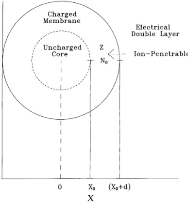
` £Å0 h£ X£

FIG. 1. A schematic representation of the structure of a particle under consideration. Z and N0are, respectively, the valence and the density of

the charged groups. The region Xú( X0/d ) represents the liquid phase,

d being the dimensionless thickness of the membrane. The region XõX0 à h0/

S

h1

X

D

/

S

h2

X2

D

. [ 2 ] denotes the rigid core of a particle; X0õXõ( X0/d ) is the ion-penetrable

membrane phase.

Substituting [ 2 ] into [1] with iÅ0 and solving the resultant

II. MODELING

expression give the electrical potential distribution for the double-layer region ( Appendix A ) ,

By referring to Fig. 1, we consider a spherical particle composed of a rigid core and an ion-penetrable, charged membrane immersed in an a :b electrolyte solution. Denote the dimensionless sizes of the rigid core and the membrane

h0Å

S

2 a

D

ln 1/[ tanh ( acd/ 4 ) ] 1 exp [0k3( X 0X00 d ) ] 10[ tanh ( acd/ 4 ) ] 1exp [0k3( X0X00d ) ] [ 3 ] as X0 and d , respectively. Here, X0Å kr0, where r0 and k

are the size of the rigid core and the reciprocal Debye length, respectively. Without loss of generality, we assume that the fixed charges in the membrane are negative and distributed

h1 Å

S

1 ak3

D

sinh

S

ah0 2

DF

tanh 2

S

acd 4

D

uniformly.

The electrical potential distribution in spherical geometry is described by the PBE

0tanh2

S

ah0 4

D

02 ln

F

tanh ( acd/ 4 ) tanh ( ah0/ 4 )

GG

[ 4 ] d2_c d X2/ 2 X d c d X Å g/iN a/b , iÅ 0, 1, [1] h2 ÅX ( h0) a sinh ( ah0/ 2 ) 8k3

F

u

*

h₀ 0 h2 1sinh ( ah0/ 2 ) X ( h0) dh0 where cÅef / kBT , gÅ[ exp ( bc )0exp (0ac ) ] , XÅkr ,

k2

Åe2

a ( a/b ) n0

a/ e0erkBT , and NÅZNAN0/ an0a. In these

expressions, f denotes the electrical potential; e is the ele- _/

*

c0

h0

uh2

1sinh ( ah0/ 2 )

X ( h0) dh0

G

, [ 5 ] mentary charge; N0and Z are, respectively, the density and

the valence of the charged groups in the membrane (0ZeNAN0 is the density of fixed charges ) ; NA represents

the Avogadro number ; erand e0are the relative permittivities where k3, u , and X ( h0) are defined in Appendix A. If the membrane is sufficiently thick, the dimensionless of the solution and the vacuum, respectively; n0

ais the

S

2 a/b

D

1 / 2

H

1 b[ exp ( bcd)01]/ 1 a[ exp (0acd)01]

J

1 / 2 0 1 X0/d

F

4 atanh

S

acd 4

DG

/ 4 ( X0/d )2 1

F

tanh 2

( acd/ 4 )02 ln [ cosh ( acd/ 4 ) ]

k3sinh ( acd/ 2 )

G

Å

S

2

a/b

D

1 / 2

H

1

b[ exp ( bcd)0exp ( bcDon) ]

/1

a[ exp (0acd)0exp (0acDon) ]

/N ( cd0cDon)

J

1 / 2 0 4 X0/d 1

H

1 atanh

F

a ( cd0cDon) 4

GJ

/ 4

( X0/d )2 FIG. 2. Schematic representation of a system containing two particles.

A2Å 0

F

4 27k3 / 2 9a4( a 2 2 02a 2 2a3)

G

tanh 2

S

acd,n 4

D

1

H

tanh2 [ a ( cd0cDon) / 4 ] 02 ln [ cosh [ a ( cd0cDon) / 4 ] ] k3sinh [ a ( cd0cDon) / 2 ] . [ 6 ] 1{ 3k3( X0,n/dn) cosh [ 3k3( X0,n/dn) ] 03k3X0,ncosh ( 3k3X0,n)

The electrostatic interaction energy between two particles

0sinh [ 3k3( X0,n/dn) ]/sinh ( 3k3X0,n) } [ 7b ]

Iel( R ) can be estimated by substituting [ 2 ] – [ 5 ] into [ B16 ] ( see Appendix B ) to yield

A3Å

F

3 32a4( 2a 2 2a30a 2 20a2)

G

tanh 4

S

acd,n 4

D

Iel( R )Å 16p ak3 3k3R

∑

2 n Å1 { Pn ,n =

∑

3 t Å1 { Atexp [ k3( 2t01 ) 1{ 5k3( X0,n/dn) cosh [ 5k3( X0,n/dn) ] 05k3X0,ncosh ( 5k3X0,n) 1( X0,n/dn0R ) ] } } , nxn*, [ 7 ] 0sinh [ 5k3( X0,n/dn) ]/sinh ( 5k3X0,n) } [ 7c ] where the subscripts n and n* denote particles n and n*,

respectively, dnis the dimensionless thickness of the mem- a₁Å

S

1

2

D

tanh 2

S

acd,n

4

D

/k3( X0,n/dn)03/

a5

a4

brane phase of particle n , and R is the dimensionless center- [ 7d ]

to-center distance between two particles ( Fig. 2 ) . The values of A1, A2, A3, and Pn ,n =are defined by

a2Åtanh 2

S

acd,n 4

D

/ln

H

1 2

F

1/cosh

S

acd,n 2

DGJ

[ 7e ] A1Å ( 3 /a1) ( X0,n/dn) cosh [ k3( X0,n/dn) ] a3Å coth ( acd,n/ 2 ) sinh ( acd,n/ 2 ) 0 1 2 0( 3 /a1) X0,ncosh ( k3X0,n)0

S

3 k3 /a1

D

1ln

H

1 2

F

1/cosh

S

acd,n 2

DGJ

[ 7f ] 1( X0,n/dn) sinh [ k3( X0,n/dn) ] /

S

3 k3 /a1

D

1X0,nsinh ( k3X0,n) a4Å600k43( X0,n /dn) [ 7g ] [ 7a ]

shown that the value of R at which Ithas its primary maxi-a5Åa 2 2a3sinh 2

S

acd,n 4

D

mum, Rmax, is Rmaxà[ b6/( b37/b26)1 / 2]1 / 3 /

F

2a2 2a3/ 1 2a 2 2/ a2

G

1sinh 4

S

acd,n 4

D

[ 7h ] /[ b60( b3 7/b 2 6)1 / 2 ]1 / 3 0b3 3 , [10 ] Pn ,n =ÅLn

F

tanh

S

acd,n = 4

DG

where 1exp [ k3( X0,n = /dn =0X0,n0dn) ] , [ 7i ] b3Åb202 D20 A132 12 D3b1 [10a ] where the energy density Lnis defined in Appendix B.

b6Å

( 9b3b4027b502b3)

54 [10b ]

The electrostatic interaction force between two particles,

fel( R ) , can be calculated by b7Å ( 3b30b2 3) 9 [10c ] fel( R )Å 0k

S

dIel d R

D

b5ÅD 2 2b2 [10d ] b4ÅD2( D202b2) [10e ] ÅkIel R / 16p ak2 3k2R

∑

2 n Å1 { Pn ,n =

∑

3 t Å1 { At( 2t0 1 ) b2Å 16p ak3 3k3b1

∑

2 n Å1 { Pn ,n =

∑

3 t Å1 { At1exp [ k3( 2t01 ) 1exp [ k3( 2t01 ) ( X0,n/dn0R ) ] } } 1( X0,n =/dn =) ] } } , nxn* [10f ] Åk( k3R /1 ) R Iel/ 32p ak2 3k2R b1Å 16p ak2 3k3

∑

2 n Å1 { Pn ,n =

∑

3 t Å1 { At( 2t01 ) 1

∑

2 n Å1 { Pn ,n =

∑

3 t Å2 { At( t01 ) _{1exp [ k3( 2t01 ) ( X0,n =/d} n =) ] } } , nxn*. [10g ] 1exp [ k3( 2t01 ) ( X0,n/dn0R ) ] } } ,

nxn*. [ 8 ] In these expressions, A132denotes the Hamaker constant, and

D2and D3are defined in [ C2c ] and [ C2b ] , respectively ( see Appendix C ) . Substituting [ 7 ] , [ C1] , [ C2e ] , [ C5a ] , and Note that if Rr `, both Ieland fel vanish, as expected.

[10 ] into [ C4 ] yields The stability ratio can be regarded as the reciprocal

colli-sion efficiency which leads to coagulation. It can be

mea-sured by the ratio of particle fluxes without and with an _{W àexp}

HF

_I

el( Rmax)0

A132D3

12 ( Rmax0D2)

GY

kBT

J

. [11] energy barrier ( 1 ) . Therefore the kinetic property can be

described by the interaction energy between two particles. According to Fuchs ( 18 ) and Overbeek ( 19 ) , the stability

The critical coagulation concentration ( CCC ) can be de-ratio of the system under considede-ration, W , can be estimated

termined by by Iel( Rc) 0 A132D3 12 ( Rc0D2) Å0 [12 ] WÅ

*

` 1

S

1 R2 r

D

exp

S

It kBT

D

d Rr, [ 9 ] fel( Rc) / kA132D3 12 ( Rc0D2)2Å0, [13 ] where RrÅR / D2, and Itis the total interaction energy

be-tween two particles. The latter includes the electrostatic re- where Rc is the dimensionless center-to-center distance be-tween two particles at the CCC. Solving these equations pulsion energy and the van der Waals attraction energy. On

TABLE 1

Average Deviation Q (%) in the Potential Distribution of the Present Perturbation Method, c, from the Exact Numerical Calcu-lation, c*a N0(M) X0 1003 511003 1002 1 3.77 4.84 5.61 2 3.13 4.27 4.85 4 2.32 3.50 4.39 6 2.17 3.28 3.96

a_{For the case ZÅ1, dÅX}

0/4, ionic strengthÅ1003M, erÅ78, and

TÅ298.15 K. t equally spaced points in the range [X0/d, X0/d/3]

are chosen, and the potentials at these points are evaluated. Q is defined by 100% [(3

aÅ1(

3

bÅ1( t

jÅ1É(c*0c)/c*]/9t, where a and b are the valences

of the cation and anion, respectively.

Rc àg/[ g( g/D2) ] 1 / 2

, [14 ]

FIG. 3. Variation of log W as a function of the radius of the rigid core of where

a particle for the case X0,1ÅX0,2ÅX0, d1Åd2ÅX0/4. — , N0Å1003M;

---, N0Å511003M; – – – , N0Å1002M. Key: erÅ78, TÅ298.15 K,

Z1ÅZ2Å1, aÅ2, bÅ1, A132Å10020J, and ionic strengthÅ1003M.

gÅD20

A132D3

12b1 . [14a ]

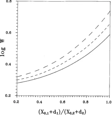
Figure 5 illustrates the variation in the stability ratio as a The CCC for counterions can be estimated by substituting

function of the size ratio of two interacting particles, ( X0,1 [14 ] into either [12 ] or [13 ] .

/d1) / ( X0,2/d2) , at a fixed mean size of two particles, [ ( X0,1

/d1) ( X0,2/d2) ]1 / 2

. This figure shows that the smaller the

III. DISCUSSION

size ratio ( the greater the difference in the sizes of two Table 1 shows the average percentage deviation in the

potential distribution estimated by [ 2 ] from the exact values, estimated by solving [1] numerically. As can be seen from this table, the performance of the present perturbation method is satisfactory.

Figure 3 illustrates the simulated variation in the stability ratio W as a function of the linear size of the rigid core of a particle at various densities of fixed charges in the membrane phase. This figure suggests that W decreases with increases of X0. This is consistent with the classic DLVO theory to-gether with the Fuchs model ( 1 ) , and the result for the case of low potential ( 16 ) . For a fixed X0, the greater the density of fixed charges N0, the greater the W . This is expected, since the greater the N0, the greater the electrostatic repulsive force between two particles.

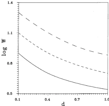
Figure 4 shows the effect of membrane thickness on the stability ratio at a constant total amount of fixed charges and particle size. As can be seen from Fig. 4, the stability ratio increases with decreases in the membrane thickness. This is because at a constant total amount of fixed charges, the

FIG. 4. Variation of log W as a function of the membrane thickness at smaller the thickness of membrane, the more concentrated

a constant total amount of fixed charges, TC, and particle size for the case the fixed charges, and the greater the electrostatic repulsion _d

1Åd2Åd , X0,1/ d1ÅX0,2/ d2Å5. — , TCÅ 2.261 10022mol;

energy. Figure 4 also suggests that the stability ratio in- - - -, TCÅ 1.13110021_{mol; – – – , TCÅ2.26110}021_{mol. Key: see}

the legend to Fig. 3. creases with the total amount of fixed charges, as expected.

where H is the dimensionless surface-to-surface distance be-tween the particle and the surface.

3.3. Two Parallel Flat Surfaces

In the case of two parallel flat surfaces, it can be shown that Iel( H )Å 8p ak4 3k 3

∑

2 n Å1

H

Ln

F

tanh

S

acd,n 4

DG

1

H

3 [10exp (0k3dn) ] exp (0k3D3H ) 0 4 27( 3k301 ) [10exp (03k3dn) ] 1

F

tanh

S

acd,n 4

DG

exp (03k3D3H )

JJ

. [17 ]

FIG. 5. Variation of log W as a function of the relative size of two interacting particles at a fixed mean size of two particles aV for the case d1

3.4. Rigid Particles and 1:1 Electrolytes

Åd2Å 1 and N0Å 811003M. — , aVÅ11; - - -, aVÅ13; – – – , aVÅ

15. Key: see the legend to Fig. 3.

For 1:1 electrolytes and rigid particles, [ 3 ] – [ 5 ] reduce to those derived by Dukhin et al. ( 20 ) .

particles ) , the smaller the stability ratio. In other words,

monodispersed particles are more stable than polydispersed 3.5. Single Particle

particles. This can be deduced from Eqs. [ C2 ] – [ C2d ] . The

Suppose that the radius of one of the two interacting parti-smaller the size ratio, the parti-smaller the value of D4, the greater

cles approaches zero, i.e., ( X0,n/dn)r0, nÅ1 or 2. Then

the absolute van der Waals attraction energy, and the smaller

dn r0 and cndoes not exist. In this case, [ 7 ] implies that

the stability ratio.

Iel( R )r 0 and Ivdwr0 by [ B2 ] . Under certain conditions, the results of the present study

can be either simplified or reduced to those reported in the

APPENDIX A

literature. We consider five special cases.

3.1. Two Identical Particles _{Substituting [ 2 ] into [1] and collecting terms of the same}

order in X , we obtain the potential distribution in the double-If the interacting particles are identical, then X0,1 Å X0,2

layer region, ÅX0, d1 Åd2Å d , cd,1Å cd,2Å cd, P1,2 ÅP2,1 ÅP ( X0, d , cd) , AtÅAt( X0, d , cd) , tÅ1, 2, 3, and [ 7 ] gives d2 h0 dX2 Å g0 /iN a/b [ A1] Iel( H )Å 32p ak3 3k3R P ( X0, d , cd) d2_h 1 d X2 0 1 a/b[ b exp ( bh0) 1

∑

3 t Å1 { At( X0, d , cd) 1exp [ k3( 2t01 ) ( X0/d0R ) ] } . [15 ] _{/a exp (0ah0) ] h1Å}02 dh0 dX [ A2 ] 3.2. A Spherical Particle and a Flat Surface

d2 h2 dX2 0 2 X dh2 dX / 2 X2h2 If particle 1 is spherical and particle 2 becomes a flat

surface, [ 7 ] reduces to 0 1 a/b[ b exp ( bh0) /a exp (0ah0) ] h2 Iel( H )Å 24p ak4 3k 3L1

F

tanh

S

acd,2 4

DG

[10 exp (0k3d2) ] Å 1 2 ( a/b ) [ b 2 exp ( bh0)0a2 exp (0ah0) ] h21, [ A3 ] 1exp [ k3( X0,1 /d10 D3H ) ] , [16 ]

where g0Åg ( h0) . The boundary conditions associated with

S

dh1 dX

D

(X0/d )/ Å 04 atanh

S

acd 4

D

[ A11]

these equations are

h£and ( dh£/ d X )r 0 as Xr `, £Å 0, 1, 2, . . . [ A4 ] h0 rcd, h£ r0 as Xr ( X0/d ) , £Å 1, 2, . . . . [ A5 ]

S

dh2 dX

D

_(X 0/d )/ Å 4 tanh2 ( acd/ 4 ) 0 8 ln [ cosh ( acd/ 4 ) ]

k3sinh ( acd / 2) . [ A12 ] Solving [ A1] with i Å 0 subject to [ A4 ] and [ A5 ] gives

[ 3 ] with

Equation [1d ] can be rewritten in terms of h£as

k3Å

H

[ ( k 02 ) k1 /2k2] / k , if k£4 [ 2k1/( k02 ) k2] / k , if kú4, [ A6 ]

S

dh0 dX

D

r 0,

S

dh£ dX

D

r0, h0r cc, and h£r 0 where k1Å2 / { k1 / 2 [ ( k / 2 )2 / ( k 02 ) 01] } , k2Å2 / k1 / 2 , and k as Xr X0,£Å1, 2, . . . . [ A13 ]

Å2/2b / a ( 17 ) . Similarly, solving [ A2 ] and [ A3 ] subject to [ A4 ] and [ A5 ] gives [ 4 ] and [ 5 ] with

Integrating [ A1] – [ A3 ] with i Å 1 subject to [ A13 ] and applying [ A5 ] , we obtain uÅ cosh ( acd/ 2 ) sinh2 ( acd/ 2 ) 0 cosh ( ah0/ 2 ) sinh2 ( ah0/ 2 )

S

dh0 dX

D

(X0/d )0 Å

F

2 a/b

G

1 / 2

H

1 b[ exp ( bcd) 0exp ( bcc) ] 0ln

F

tanh ( ah0/ 4 ) tanh ( acd/ 4 )

G

[ A7 ] /1 a[ exp (0acd)0exp (0acc) ] X ( h0) Å 1 2k3ln

FS

cosh ( ah0/ 2 ) /1 cosh ( ah0/ 2 ) 01

DS

cosh ( acd/ 2 )01 cosh ( acd/ 2 )/1

DG

/N ( cd0 cc)

J

1 / 2 [ A14 ] /X0 /d . [ A8 ]

S

dh1 dX

D

(X₀/d )0 Å 0 4 atanh

S

a ( cd 0cc) 4

D

[ A15 ]

Substituting [ 3 ] – [ 5 ] into [ 2 ] gives the potential distribu-tion in the double-layer region. For 1:1 electrolytes, [ 3 ] – [ 5 ] reduce to the results proposed by Dukhin et al. ( 20 ) .

Differentiating [ 2 ] with respect to X and applying [ A5 ] ,

S

dh2

dX

D

(X0/d )0 Å 4 tanh2 ( a ( cd0cc) / 4 ) 08 ln [ cosh ( a ( cd0cc) / 4 ) ] k3sinh ( a ( cd0cc) / 2 ) . [ A16 ] we obtain

S

d c d X

D

_X 0/d Å

∑

` £Å0

FS

dh£ dX

DY

X £

G

X0/d If the membrane phase is sufficiently thick, there is no net

charge as XrX0, and c approaches cDon, the dimensionless Donnan potential. In this case, letting iÅ 1 in [1] yields

à

S

dh0 dX

D

X0/d / 1 X0/ d

S

dh1 dX

D

X0/d _{g ( c} Don)/N Å0. [ A17 ]

cDoncan be estimated by solving this equation. On the basis

/ 1

( X0 /d )2

S

dh2

dX

D

X0/d

. [ A9 ]

of [1b ] , [ A9 ] , [ A10 ] – [ A12 ] , and [ A14 ] – [ A16 ] , [ 6 ] can be recovered.

Integrating [ A1] – [ A3 ] with i Å 0, subject to [ A4 ] and

APPENDIX B

employing [ A5 ] , we have

Let E be the strength of electric field. We have

S

dh0 dX

D

(X0/d )/ Å

F

2 a/b

G

1 / 2

H

1 b[ exp ( bcd)01] _{Ç r( fE )ÅfÇrE/ErÇf, [ B1]}

whereÇ _{is the differential operator. Since EÅ 0Çf, the} /1

a[ exp (0acd)01]

J

1 / 2

[ A10 ]

Ç rEÅ 0 ÇrÇf Ft elÅ 0

S

e0er 2

D

*

A fErn d A01 2

*

V1 rfixfd V1, [ B9 ] Å 0[( M £Å1z£en 0 £exp (0z£c )0irfix] e0er , [ B2 ]

where n denotes the unit outer normal vector of surface where n0

£ and z£denote, respectively, the number concentra- element d A . Since both E and f are continuous, and fE is

tion of the£_{th ion species in the bulk liquid phase and its bounded, the surface integral in [ B9 ] vanishes, and we have}

valence, M is the number of ion species, and rfixrepresents the density of fixed charges evaluated by

Ft elÅ 0

1 2

*

V1

rfixfd V1. [ B10 ]

rfixÅZeNAN0. [ B2a ]

For a rigid surface E is not continuous at the solid – liquid For the present system, the density of internal energy, uel, _{interface. Thus, if n is parallel to E , letting V1Å0 in [ B9 ]} is identical to the electric field energy, i.e., _{leads to}

uelÅ

S

e0er

2

D

ErE . [ B3 ] FtelÅ

sf0A

2 , [ B11]

where f0denotes the surface potential, and A is the area of For dilute solutions the density of entropy, sel, is

the surface.

The electrostatic energy of a system containing K

parti-selÅ 0

S

kB 2

D

∑

M £Å1 n£ln

S

n£ n0 £

D

, [ B4 ] cles, Iel( R ) , can be calculated by

Iel( R )ÅFtel( R )0Ftel(`) , [ B12 ] where n£is the number concentration of species£. According

to the Gibbs – Helmholtz equation, we have _{where R is the set of distances Rn ,n =, n , n* Å1, 2, . . . , K , n}

xn*, Rn ,n =being the dimensionless center-to-center distance

felÅuel0Tsel, [ B5 ] between particle n and n*, with Rn ,n = ÅRn =,n. Suppose that

the double layer around a particle is thin. Employing [ B10 ] where felis the density of electrical free energy. Substituting and [ B2a ] , we obtain

[ B3 ] and [ B4 ] into this expression, employing the Boltz-mann distribution law for ions, and using [ B1] and [ B2 ] ,

Ft el( R )Å

∑

K n Å1

*

V1,n Lncd V1,n [ B13a ] we have Ft el(`) Å

∑

K n Å1

*

V1,n Lncn ,i Å1d V1,n [ B13b ] felÅ 0

S

e0er 2

D

Çr( fE ) 0 irfixf 2 . [ B6 ]

Denote the volume of the membrane phase and that of the liquid phase as V1 and V2, respectively, and let V Å V1 /

V2. The total free energy of the system, F t el, is cÅ cn ,i Å1/

∑

n = cn =,i Å0, X0,nõXnõ( X0,n/dn) , n , n* Å1, 2, . . . , K , n* xn cn ,i Å0/

∑

n = cn =,i Å0, ( X0,n/dn)õXn, ( X0,n =/dn =)õXn =, n , n* Å1, 2, . . . , K , n* xn , [B14] Ft el Å

*

feld V . [ B7 ]

Substituting [ B6 ] into [ B7 ] gives

where LnÅ 0znNAN0, n kBT / 2, d V1,nÅ2pX 2 nsin und Xndun/ Ft elÅ 0

S

e0er 2

D

*

V Çr( fE ) d V 01 2

*

V1 rfixfd V1, [ B8 ] _k3_{, and u}

n is the angle between line segments defined by

Rn ,n = and Xn. Ftel(`) is the electrostatic free energy for the case any pair of two particles are infinitly apart. Since cn ,i Å1

is a function of Xn, Ftel(`) is independent of R. For a system where d V and d V1represent volume elements. Applying the

ftÅ 0

S

k D3

DS

dIt dH

D

cÅ c1,i Å1/c2,i Å0, X0,1õX1õ( X0,1/d1) c1,i Å0/c2,i Å0, ( X0,1/d1)õX1, ( X0,2/d2)õX2 c1,i Å0/c2,i Å1, X0,2õX2õ( X0,2/d2) . [ B14a ] Å fel0

S

k D3

DS

dIvdw dH

D

. [ C3 ]

The stability ratio of the system, W , can be estimated by By referring to Fig. 2, we have [ 9 ] . As an approximation, the total interaction energy is replaced with its primary maximum, It,max, and the integra-tion procedure suggested by Overbeek ( 19 ) leads to

X1Å ( R 2 /X2 20 2 RX2cos u2) 1 / 2 [ B15a ] X2Å ( R 2 /X2 102 RX1cos u1) 1 / 2 , [ B15b ] W àexp

S

It,max kBT

D

. [ C4 ]

where R denotes the dimensionless center-to-center distance between two particles, and the angles u1and u2are defined

in Fig. 2. For a two-particle system, [ B12 ] becomes _{As Hr0, [ C2 ] reduces to}

Iel( R )Å

∑

2 n Å1

*

V1,n = Lncn =,i Å0d V1,n =, n* x n . [ B16 ] IvdwÅ 0A132 12H [1/H ( 1 0D4) /2H ln H/ rrr] APPENDIX C à0A132 12H . [ C5a ]

The total interaction energy Itincludes the van der Waals

energy Ivdwand the electrostatic energy Iel, i.e., _{If the size of one of the two interacting particles approaches} infinity, i.e., X0,n r `, nÅ1 or 2, [ C2 ] reduces to

ItÅIvdw/Iel. [ C1] IvdwÅ 0A132 6

F

1/2H 2H ( 1/H ) /ln

S

H 1/ H

DG

. [ C5b ] We assume that ( 1 ) IvdwÅ 0A132 12H

F

1 1/D4H / H

1/H/D4H2 If the sizes of two interacting particles approach infinity, the problem reduces to the interaction of two parallel planar surfaces. In this case, [ C2 ] gives

/2H ln

S

H/D4H 2 1/H/D4H

2

DG

, [ C2 ]

IvdwÅ 0A132Ap[12p( D3H )2] , [ C5c ] where Ap is the average surface area of two particles, and where

D3H represents the dimensionless surface-to-surface distance between two particles.

D4Å

D3

2 D2 [ C2a ] At the critical cogulation contration,

ItÅ0 and ftÅ 0. D3Å D1 D2 [ C2b ] ACKNOWLEDGMENT D2Å X0,1 /d1/X0,2 /d2 [ C2c ]

This work was supported by the National Science Council of the Republic

D1Å 2 ( X0,1/d1) ( X0,2 /d2) [ C2d ]

of China under Grant NSC84-2214-E002-030.

HÅ ( R0D2)

D3

, [ C2e ]

REFERENCES

1. Hunter, R. J., ‘‘Foundations of Colloid Science,’’ Vol. I. Oxford Univ. where A132denotes the Hamaker constant and D3represents _{Press, London, 1989.}

the dimensionless reduced radius. The interaction force be- 2. Hiemenz, P. C., ‘‘Principles of Colloid and Surface Chemistry,’’ 2nd ed. Dekker, New York, 1986.

3. Wiese, G. R., and Healy, T. W., Trans. Faraday Soc. 66, 490 ( 1970 ) . 13. Kawahata, S., Ohshima, H., Muramatsu, N., and Kondo, T., J. Colloid Interface Sci. 138, 182 ( 1990 ) .

4. Metcalfe, I. M., and Healy, T. W., Faraday Discus. Chem. Soc. 90,

335 ( 1990 ) . 14. Terui, H., Taguchi, T., Ohshima, H., and Kondo, T., Colloid Polym. Sci. 268, 76 ( 1990 ) .

5. Overbeek, J. Th. G., Pure Appl. Chem. 52, 1151 ( 1980 ) .

6. Donath, E., and Pastushenko, V., Bioelectrochem. Bioenerg. 6, 543 15. Taguchi, T., Terui, H., Ohshima, H., and Kondo, T., Colloid Polym. Sci. 268, 83 ( 1990 ) .

( 1979 ) .

7. Wunderlich, R. W., J. Colloid Interface Sci. 88, 385 ( 1982 ) . 16. Hsu, J. P., and Kuo, Y. C., J. Chem. Phys. 103, 465 ( 1995 ) . 17. Hsu, J. P., and Kuo, Y. C., J. Chem. Soc. Faraday Trans. 91, 1223 8. Levine, S., Levine, M., Sharp, K. A., and Brooks, D. E., Biophys. J.

42, 127 ( 1983 ) . ( 1995 ) .

18. Fuchs, N., Z. Phys. 89, 736 ( 1934 ) . 9. Sharp, K. A., and Brooks, D. E., Biophys. J. 47, 563 ( 1985 ) .

10. Reiss, H., and Bassignana, I. C., J. Membrane Sci. 11, 219 ( 1982 ) . 19. Overbeek, J. Th. G., in ‘‘Colloid Science’’ ( H. R. Kruyt, Ed.) , Vol. 1. Elsevier, Amsterdam, 1952.

11. Selvey, C., and Reiss, H., J. Membrane Sci. 23, 11 ( 1985 ) .

12. Seaman, G. V., in ‘‘The Red Blood Cells’’ ( D. M. Sergenor, Ed.) , 20. Dukhin, S. S., Semenikhin, N. M., and Shapinskaya, L. M., Dokl. Phys. Chem. 193, 540 ( 1970 ) .