A novel radial basis function network classifier with centers set by hierarchical clustering

Proceedingsof International Joint ConferenceonNeuralNetworks,Montreal, Canada,July31-August4, 2005

A

Novel Radial

Basis

Function

Network

Classifier

with

Centers

Set

by

Hierarchical

Clustering

Yu-Yen Ou and Yen-Jen Oyang

Department ofComputer Science and Information Engineerin National Taiwan University

Taipei, Taiwan

E-mail: {yien,yjoyang}(csie.ntu.edu.tw

Abstract-Thispaper proposes a novel methodto construct a

radial basisfunction network(RBFN)classifier.Ourcontribution

consistsof two parts.The firstoneisanincrementalhierarchical clustering algorithm for constructing the hidden layer, and the

second oneis toimprovetheleast mean squareerrormethodthat

calculates theweights between the hidden and the output layers

of an RBFN. This paper discusses the effects ofincorporatingan

incremental hierarchical clustering algorithm for constructing

an RBFN optimized for data classification applications. The formation of clusters is controlled bythe class labels oftraining

samples and therefore the clusters identified are well adapted

to the local distributions of training instances. In addition,

the incremental framework largely reduces the requirement of

memory space when the trainingdata set is large. In regard to thecalculation ofweights, we employ the regularization theory

to solve the singular matrix problem that might happen in

determiningtheoptimal weights. Experimentalresultsshow that the dataclassifier constructed is capable ofdeliveringcomparable classification accuracy as the support vector machine (SVM)

and the kernel density estimation based classifier that we have recently proposed, while enjoyingsignificant executionefficiency

inhandlingdata setsthatcontainsahighpercentageof redundant training instances.

I. INTRODUCTION

The radialbasis function network (RBFN) is a specialtype

ofneuralnetworks with several distinctive features [1], [2], [3], [4], [5], [6]. Since its first proposal, the RBFN has attracted

ahigh degree of interest in research communities. An RBFN

consists of three layers, namely the input layer, the hidden layer, and the output layer. The input layer broadcasts the

coordinates of the input vector to each of the nodes in the hidden layer. Each node in the hidden layer then produces

an activation based on the associated radial basis function. Finally, eachnode inthe outputlayercomputes alinear

com-binationoftheactivations of the hidden nodes. Howan RBFN reacts to agiven input stimulus is completely determined by theactivation functions associated with the hidden nodes and

theweights associated withthelinks between the hidden layer and the output layer. The general mathematical form of the outputnodes in an RBFN is as follows:

k

cJ(x)

=

Ewji

.(llx

- i

(I1

)

i=1

Chien-Yu Chen

Ig Graduate School ofBiotechnology and Bioinformatics

Department ofComputer Science and Engineering

Yuan Ze University, Chung-Li, Taiwan E-mail: [email protected]

where

cj(x)

is the function corresponding to thej-th output unit (class-j) and is a linear combination of k radial basis functions

¢()

with centerpi and bandwidthvi. Also, wjis the

weight vectorofclass-j and

wji

is the weight corresponding

to the j-th class and i-th center. The generalarchitecture of RBFNis shown in Fig 1.

In this paper, we select the spherical (or symmetrical)

Gaussian functionas ourbasis function ofRBFN, so the Eq.1

becomes:

k

(

lix-i

cj

(x)

=

1wji

exp -

2oc?

i1l I

(2)

From Eq.2, we can see that constructing an RBFN involves determining the number ofcenters,k,thecenterlocations,

,ui,

the bandwidthofeach center,vi,andtheweights,

wji.

Thatis, trainingan RBFNinvolvesdeterminingthevalues ofthree sets of parameters: the centers

(pi),

the bandwidths

(ai),

and the

weights

(wji),

in order tominimize a suitable cost function. Basically, there are two categories of learning algorithms proposed for RBFNs [5], [7]. The first category oflearning algorithms simply places one radial basis function at each sample [8], [9]. On the other hand, the second category of learning algorithms attempt to reduce the number of hidden nodes in the network, or equivalently the number ofradial

basis functions in the linear function above [10], [11], [12],

[13], [14]. One primary motivation behind the design ofthe second categoryofalgorithms is to reduce the complexity of

the network constructed. The typical procedure incorporated in the second category of learning algorithms conducts a

clustering analysis onthetraining instancesandthenallocates

one hidden node foreach cluster of instances. In thisregard,

the effects of a wide variety of clustering algorithms have

beeninvestigated [4], [15]. Nevertheless, boththe conventional

agglomerative hierarchical clustering algorithm and the

con-ventional partitional algorithm suffersome kinds of

deficien-cies. The mainproblem with the conventional agglomerative

hierarchical clustering algorithm is its space complexity of

0(n2),

wherenis the number oftraining instances, duetothe need to store pairwise distances or similarity scores between thetraining instances.The mainproblemwiththe conventional

InputLayer Hidden Layer Output Layer

Fig. 1. GeneralArchitecture of RadialBasisFunctionNetworks

out how many clusters are appropriate for the given training dataset.

In 1997, Hwang et al. [12] proposed an incremental

clus-tering based approach for determining the locations of hid-den nodes in the RBFN to be constructed. The incremental

approach enjoys several advantages. First, it doesnot needto

computeall thepairwise distancesorsimilarityscoresbetween training instances. The key issue in this regard isthatthespace complexity for storing the pairwise distances or similarity

scoresisgreatlyreduced, in additiontolower timecomplexity.

Second, it figures out the number of clusters automatically

based on a user-specified parameter. Third, it executes more

efficiently than the conventional agglomerative hierarchical clustering algorithm and the conventional partitionalclustering algorithm. Nevertheless, the incremental clustering algorithm proposed by Hwang employs a fixed threshold ofradius to control the formation of clusters. As a result, the clusters identified may not be well adapted to the local distributions of training instances. For example, in a region with a low local density of training instances, the threshold of radius for controlling the formation of clusters should be set to a large value. On the otherhand, in a region withahigh local density oftraining instances, the threshold of radius should be set to

a small value.

This paper proposesa novel method to construct an RBFN classifierby usinganincremental hierarchical clustering algo-rithm for constructing an RBFN optimized for data classifica-tion applications. Our contribution consists of two parts. The first one is an incremental hierarchical clustering algorithm

that constructs the hidden layer effectively and efficiently. Since the clustering algorithm is hierarchical, the formation of clustersis controlled by the class labels of training samples instead ofafixed threshold and therefore the clustersidentified

arewelladapted to the localdistributions of training instances.

In addition, because the clustering algorithm is incremental, it does not need to compute all the pairwise distances or

similarityscoresbetween training instances. The second part is

animproved leastmeansquare errormethod that calculates the

weightsbetween the hidden and theoutputlayers ofanRBFN.

In [12], authors proposed an improved method which uses a

smaller matrix to computethe weights. The methodproposed

by [12] ismoreefficient and practical than the traditionalone,

but it may suffer the singular matrix problem and fails to buildthe classifier in suchcase. We solve the singular matrix problem byusing the regularization theory in this paper, and then propose a method that can obtain the optimal weights analytically and efficiently.

Experimental results show that the data classifier

con-structed is capable of delivering comparable classification

accuracy as the SVM [16] and the novel kernel density

estimation (KDE) based classifier that we have recently

pro-posed [8], while enjoying significant execution efficiency in handlingdata sets that contains ahighpercentageofredundant training instances. For example, in the experiment with the shuttle data set in the UCI repository [17], the mechanism proposed in this paper enjoys 1231 times and 259 times

speedup overthe SVM andthe KDE based classifier that we

have recently proposed, respectively, for constructing a data classifier. In addition, the mechanism proposed in this paper

delivers comparable execution efficiency as the SVM in the prediction phase andenjoys 481 times speedupovertheKDE based classifier in this regard. Experimentalresults alsoreveal

that the approaches that have been proposed in recent years

for solving the efficiency issues of the SVM and the KDE based classifier alllead to slight degradation of classification accuracy.

This paper is organized as follows. In next section, we introduce anincremental clustering method.InSectionIIIand

IV, wedetailhow to calculate the bandwidths and weights of

theradialbasis functions which areemployed in constructing theRBFN. Next, numericalexperiments are shown in Section

V. Finally, we have some discussions and conclusions in Section VI.

II. DETERMININGTHECENTERS

In the proposed hierarchical approach, a hierarchical ag-glomerative clustering (HAC) algorithm [18], [19] is invoked to cluster all the instances in training data set. After hier-archical clustering terminates, the class labels are applied

to the dendrogram to derive target clusters. Each node in the clustering dendrogram corresponds to a cluster of data instances. A node in the dendrogram is identified as a target cluster if it contains only data instances from a single class and its parent does not satisfy the criterion. The centroids of the target clusters are used as the centers in constructing the hidden layer of RBFN. In this paper, the complete-link algorithm [19] is employed. The reason of employing the complete-link algorithm is its tendency to find spherical clusters. Since the hierarchical clustering algorithms suffer higher time complexity, an incremental clusteringframework forexpeditingthe hierarchical clustering process is introduced

A. Incremental framework

We adopt the incremental framework proposed in our pre-vious work [20]. This section describes how the incremental

algorithm works. The incremental algorithm operates in two

phases, initialphase and incrementalphase. Inbothphases, it

invokes the complete-link algorithm to construct a clustering dendrogram.

1) Initialphase: Inthe incrementalalgorithm,it is assumed

that all the incoming data instances are first buffered in an

incoming data pool. In the first phase of the algorithm, a

number of data instances are taken from the incoming data

pool and the complete-link algorithm is invoked to cluster

these instances build a tentative dendrogram. We can assume

that these datainstances areselectedsequentially accordingto

theorder ofinput sequence. As demonstrated in ourprevious work [20], the proposed incremental frameworkemploys two

operations, split and merge,toreduce the influencefrominput ordering. When the complete-linkalgorithmterminates, target clusters are derived by the method described above, i.e. the class labels areused to identify the cluster boundaries in the clustering hierarchy.

Thereare fourpieces of information recorded for each target cluster: (1) the centroid, (2) theradius, (3) the class label and (4) the number of instances in the cluster. The radius ofa

cluster is defined to be the maximum distance between the centroid andthe data instances in this cluster.

2) Incremental phase: In the second phase of the incremen-talalgorithm, thedatainstances remained in theincoming data pool are examined one by one. For each new data instance,

thealgorithm willfind its nearest neighborinthe setof target clusters. If the distance between thenewdata instance and its

nearest target cluster is smaller than the radius of the target cluster, thenewdatainstance is inserted into the target cluster. If not, the data instance is currently an outlier to the set of target clusters and is therefore put into the tentative outlier buffer temporarily. The data instance, however, may form a

target cluster with other data instances that are already in the tentative outlierbuffer or that come in later.

If a data instance is successfully inserted into an existing target cluster, we should check if the new data instance possesses the same class label with the other data instances

in the target cluster. If not, an additional operation called split should be invoked to identify new target clusters in this local area. In the split operation, we apply the complete-link

algorithm onlyto the datainstances in this target cluster, and identify new target clusters with pure property as we did in the first phase. After the split operation finishes, the number of target clusters will increase at least by one.

Once the number of data instances in the tentative outlier buffer exceeds a threshold, the complete-link algorithm is invoked again to construct a new tentative dendrogram. In this reconstruction process, the primitive objects are the target clusters and the data instances in the tentative outlier buffer.

In this case, each target cluster is represented by its centroid and regarded as asingle data instance. When a new tentative dendrogram has been generated, the same procedure and

criterioninvoked in the firstphaseareinvokedagaintofind the

targetclusters from the newtentativedendrogram.During the reconstruction process, two original target clusters will have chance to form a new bigger target cluster. This is regarded

as the so-calledmerge operation.

The incremental phase repeats until there is no data

in-stances left in the incoming data pool. After the clustering

process terminates, the centroids of all the target clusters

are collected as the centers of RBFN when constructing the classifier in the following sections.

III. CALCULATIONOFTHEBANDWIDTHS

For the hidden layer of the RBFN classifier, we use the proposed hierarchical approach to determine the number of the nodes andtheircenter locations. Anotherparameter tobe decided for each node in the hiddenlayer is the bandwidth of its kernel function,oi.Here, weemploythe methodpresented by Moody and Darken [21] to determine the bandwidth of each kernel function. The bandwidth ofa kernel function is

set as /denemy, where denemy is the distance to the center

of the nearest cluster which belong to a different class and

,3

is a constant. In this paper, we follow the heuristic setting suggested by [12], i.e. ,3 = 5.

IV. CALCULATIONOF THEWEIGHTS

After the centers and bandwidths of the kernel functions

in hidden layer have been determined, the transformation

between theinputsandthecorresponding outputsofthehidden units is now fixed. The network can thus be viewed as an

equivalent single-layer network with linear output units. Then,

we use the least mean square error method to determine the

weights associated with the links between the hidden layer and

the output layer.

Inthissection,wewillshow how the least mean square error method have been used in data classification field, and then propose a method which has a better theoretical foundation and practical use.

Assume h is the output of the hidden layer.

(3) where k is the number of centers, Xl(x) is the output value

of first kernel function with input x. Then, the discriminant function

cj(x)

ofclass-j can be expressed by the following:

ca(x)=wTh, j=1,2,...,m

₍₄₎

wherem is the number of class, and wj is the weight vector

ofclass-j. We can show

wj

as:

Wj =

[

Wjl Wj2 * * * Wjk ].

(5)

After calculating the discriminant function value of each class, we choose the class with the biggest discriminant function valueasthe classification result. We will discuss how to get the weight vectors by using least mean square error method in thefollowing subsections.

A. Traditional LeastMeanSquare Error Method

The traditional least mean square error method was pro-posedbyBroomhead and Lowe[22].This method isoriginally

proposed for function approximation, and is themostpopular supervised learning method of constructing the weights of RBFN [2],[3],[5], [23]. Inthismethod,theobjectivefunction ofclass-j can be shown as:

n

minE

[cj (Xi)

-Vj

(Xi)

2

i=l

where

ifx E class-j,

otherwise.

This system is overconstrained, beingcomposedofn equa-tions with k unknown weights, then the optimal solution of

w; can be writtenas

3

Yi,

(8)

where

yj

= [

vj(xl) vj(x2)

...

vj(x-)

]T,

4Dli

=

qi(xi)

and 4.+ is the pseudoinverse of4.. The matrix 4. is

rectangular (nxk) and itspseudoinverse canbecomputed as (+ - (4DT4D)-114T

provided that (4DT4D)1- exists. The matrix

(4.T4.)

is square and its dimensionality is k, so that it can be inverted in time proportional to k3.

Although in theory thequantity of(.T4.)-1 exists,thecost

ofcomputing4.+ isveryhigh. First,weneedto store4.of size

(nx k) in thememory. The value ofnin some classification problems is very large, such that it may beimpracticaltohave such large amounts ofmemory space for storage. Also, the processofcalculating

(.T4.)-1

forlarge 4. iscomputationally

expensive.Inaddition,this method needsalotofcomputations

for matrixmultiplicationandinversion.Therefore,this method maynot be suitable for the use ofclassification problem.

B. ImprovedLeastMean Square Error Method

The improved least mean square error method for data classification was proposed by Devijver et. al.[24] and has been employed by Hwang et. al. in [12]. This method aims

tocalculate

wj

for m classes at the same time. We detail the procedures as follows.

For aclassification problemwithmclasses, letVi designate the i-th column vector ofan m x m identity matrix and W be an k xm matrix of weights:

W'=[W I W2 ... Wi ].

Then theobjective function to be minimized is

m

j(W) = E

pE

{Vil },

j=l (10)

where

Pj

and

Ej

{} are the a priori probability and the expected value ofclass-j, respectively.

(6)

Tofind theoptimal W that minimizes J,wesetthe gradient ofJ(W) to be zero:

m m

VwJ(W) =2 E

PjEj

{hhT} W-2

E

PjEj

{h}

VjT

= [0],

j=1 j=1

(1 1)

where [0] is a k xm null matrix.

Let Ki denote the class-conditional matrix ofthe second-ordermoments of h, i.e.

Ki

=

Ei

{hhT}.

(12)

If K denotes the matrix of the second-order moments under (7) the mixture distribution, we have

m

K=

E

PjKj.

j=l

(13)

Then Eq. 11 becomes

KW = M, where (14) m

M=EP3Ej{h}VfT.

j=l (15)

If K is nonsingular, theoptimal W canbe calculated by

W*

=K-1M.

₍₁₆₎

When compared to the traditional method, the size ofK,

k x k, is much smaller than the 4. matrix of size (n x k) described intheprevious subsection. Therefore, the improved

method requires less memory space for storing the matrix,

as well as consumes much less computation time for matrix

multiplication. It isapparentthattheimproved method ismore

efficient than the traditional one.

However, there is a critical drawback of the improved

method. That is, K may be singular and this will crash the wholeprocedure. Byobserving the matrix hhT, we are aware

of that the matrix hhT is symmetric positive semi-definite (PSD) matrix with rank = 1. Since K is the summation of

hhT foreachtraining instance, K is also a PSD matrix with

rank < n. When k -÷ n, it is highly possible to have K be singular. From ourexperiences, if all the training instances are chosenascenters, this method is not going to work eventually. Thus, we solved this problem in the following subsection. C. ProposedLeast Mean Square Method

A very simple solution to solve the singular problem has

been shown in the context ofregularization theory [25]. It consists inreplacing the the objective function as follows:

m m

J(W)=EP,PjE;i{|IWTh-jII}+

+A

E

wfw

(17)

j=1 j=1

where A is the regularization parameter. Then the Eq. 14

becomes

(K+AI)W= M. (18)

1

TABLE I

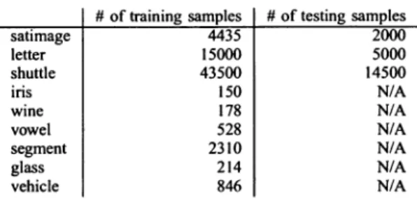
THEBENCHMARK DATASETSUSED INTHEEXPERIMENTS

satimage letter shuttle iris wine vowel segment glass vehicle

#oftraining samples # oftesting samples 4435 15000 43500 150 178 528 2310 214 846 TABLE II

COMPARISONOFCLASSIFICATIONACCURACYWITH THETHREELARGER DATASETS 2000 5000 14500 N/A N/A N/A N/A N/A N/A

KDE SVM INN 3NN APC-1II Proposed

satimage 92.30 91.30 88.80 90.65 90.25 92.00

letter 97.12 97.98 95.68 95.16 91.16 97.48

shuttle 99.94 99.92 99.94 99.91 97.34 99.82

Average 96.45 96.40 94.84 95.24 92.92 96.43

TABLE III

COMPARISONOFCLASSIFICATIONACCURACYWITHTHESIXSMALLER DATASETS

If we set A > 0, (K+ AI) will be a positive definite (PD)

matrix and therefore is nonsingular. The optimal W* can be

calculated by

W* = (K +

AI)

1M. (19)

Finally, we can get the optimal

wj*

for class-j from W*, and then the optimal discriminant function

cj(x)

for

class-j is derived. By using the regularization theory, the optimal

weights can beobtained analytically and efficiently.

V. EXPERIMENTSIN THEPROBLEM OF DATA CLASSIFICATION

The experiments in this section are conducted to evaluate the performance of the proposed RBFN classifier against other famous classifiers, the KDE based classifier [8], SVM

[16], and KNN. Also, the incremental hierarchical clustering

algorithm is compared with the APC-III clustering algorithm

employedin[12].OurproposedRBFNclassifierand the

APC-III based classifier share the sameprocedures ofdetermining

bandwidths and weights in constructing the RBFN. The dis-cussions of the experiments will focus on the following two

issues: classification accuracy and execution efficiency. TableIlists main characteristics of the nine benchmark data

setsused in the experiments. All these data sets are from the

UCIrepository [17]. Among thenine datasets, three ofthem are considered asthe larger ones, as eachcontains more than 5000 samples with separate training and testing

subsets.

The

remaining six datasetsareconsidered asthe smalleronesand there are no separate training and testing subsets in these six smaller data sets. Accordingly, different evaluation practices have beenemployed for the smaller data sets and for the larger datasets. Forthe threelarger data sets, 10-fold cross validation has been conducted on the training set todeterminetheoptimal parameter valuestobe used in thetesting phase. Onthe other hand, forthe six smaller data sets, 10-fold cross validation has been conducted on the entire data set and the average result is reported.

Ourincrementalalgorithm has two keyparameters, the size of initial data samples and the size of the tentative outlier buffer. In our experiments, both of the size of initial data instances and the size of tentative outlier buffer are set to 1000.

Weobservedthatthese two buffers do not affect the quality of the classifier much but do influence the execution time. The larger thebuffersize,thelonger the reconstructing process. In theexperiments, the incremental mechanism isturnedonwhen

KDE SVM INN 3NN APC-III Proposed

iris 97.33 97.33 96.00 95.33 95.33 96.00 wine 99.44 99.44 95.52 96.07 98.89 97.78 vowel 99.62 99.05 99.62 97.35 93.37 98.48 segment 97.27 97.40 97.27 96.14 94.98 97.53 glass 75.74 71.50 72.01 92.01 69.16 72.86 vehicle j 73.53 86.64 69.73 71.39 78.25 79.19 Average 90.49 91.89 88.36 88.05 88.33 90.31

the size oftraining data set is largerthan 20000. Inregard to

the parametersettings ofother classifiers for comparison, we

adopted the parameter settings suggested by the authors in their original papers.

Table II compares the accuracy delivered by alternative classification algorithms with the threelargerbenchmarkdata

sets. As Table 1I shows, the proposedmethodbasically deliver

thesame level ofaccuracywithother famousclassifiers, SVM

and KDE, while the KNN and APC-III based classifier do

notproduce comparable generation results. Table III lists the

experimental results with the six smaller data sets. Table III shows that the proposed method basically deliver the same

level of accuracy for these six data sets. The experimental results presented in Table III also show that the proposed method, KDE based classifier and the SVM generally deliver

a higher level of accuracy than the KNN andAPC-III based classifier.

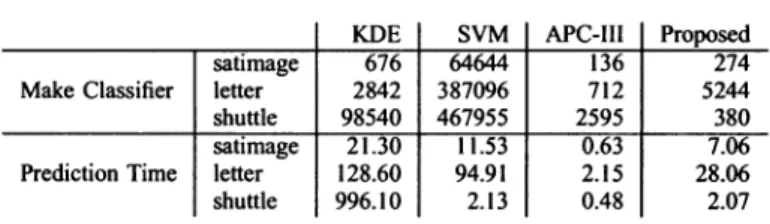
Table IV compares the execution time of the KDE based classifier, the SVM, the APC-III based classifier and the

proposed method with the three larger data sets presented

in Table I. In Table IV, the total time taken to construct classifiers based on the given training data sets are listed

in the rows marked by "Make classifier". The time listed in "Makeclassifier"row arethe timeofcrossvalidation forKDE

based classifier and the time of model selection for SVM.

On the other hand, for both the APC-III based classifier and theproposed algorithm, the reported time include the time of

clusteringprocess and the time ofcalculting bandwidths and weights. In addition, the time taken by alternative classifiers

to predict the classes of the testing instances are listed in the

rows marked by "Prediction".

As we can see in Table IV, the mechanism proposed in thispaper is much more efficient than the SVM and the KDE based classifier for constructing a data classifier. In addition, the mechanism proposed in this paper delivers comparable execution efficiency as the SVM in the prediction phase and

TABLE IV

COMPARISONOFEXECUTIONTIMEINSECONDS

KDE SVM APC-III

0satimage 676 64644 136 274 Make Classifier letter 2842 387096 712 5244

shuttle 98540 467955 2595 380

_ -* 1%. e^ 11 t I ^ 1.

Prediction Time satimageletter shuttle 21.30 128.60 996.10

11.53

94.91 2.13 0.63 2.15 0.48

enjoys

30 times

speedup

overthe KDEbased classifier in this

regard.

VI. CONCLUSION

In thispaper wepresentan efficient method toconstruct an

RBFNclassifierwhose

performance

was shownto be as good

as the

existing

classification methods on the data sets used

in this paper. Our contribution consists of two parts. First,

we propose an incremental hierarchical clustering algorithm

for

constructing

the hidden

layer

effectively and efficiently.

Second,

an

improved

least mean square error method that

calculates the

weights

between the hidden and the output

layers

ofan RBFN is introduced.

Inthe

proposed

clustering

approach, theformation of

clus-ters is controlled

by

the class lables oftraining samples and therefore the clusters identified are well adapted to the local

distributions of

training

instances. In addition, it does not

need tocomputeall the

pairwise

distances orsimilarity scores

between

training

instances. Experimental results show thatthe data classifier constructed is capable ofdelivering comparable

classification accuracy as the SVM and the kernel density

estimation based classifier that we have recently proposed,

while

enjoying

significant

execution efficiency in handling

datasets thatcontains ahighpercentage of redundant training

instances.

Also,

the

proposed

least mean square error method is

efficient and with

good

theoreticalfoundations. Thetraditional

least mean square method requires large memory to store the

matrix and consumes a lot of execution time for the matrix

multiplications

andinversions.Theimproved method-proposed

by [12]

ismoreefficient andpractical than thetraditional one,

but it may suffer the

singular

matrix problem and fails to

build the classifier in such case. In this paper, we solve the

singular

matrix

problem

by

usingtheregularizationtheory,and

this

provides

a

good

framework forconstructing anRBFNin

classification

problems.

Experimental

results also reveal that the approaches that

have been

proposed

inrecent years for solving the efficiency

issues of the SVM and the kernel density estimation based

mechanism all lead to slight degradation of classification accuracy.

Thus,

howtoimprovetheefficiency oflearning

algo-rithms without

sacrificing

classification accuracy stilldeserves

further

studies.

[2] T. Poggio and F. Girosi, "A theory of networks for approximation and learning,"Tech. Rep. A.I. Memo 1140, Massachusetts Institute of

Technology, ArtificialIntelligence Laboratoryand Center forBiological Information Processing, WhitakerCollege,Jul 1989.

[3] J.Ghosh andA.Nag,"Anoverview of radial basisfunction networks," RadialBasis Function Neural Network

Theory

andApplications, R.J.

Howlerr and L. C. Jain (Eds), 2000.

[4] T. M. Mitchell, MachineLearning. McGraw-Hill, 1997.

[5] M. J. L.Orr,"Introduction toradialbasis functionnetworks,"tech.rep.,

Center forCognitive Science,UniversityofEdinburgh, UK, 1996.

[6] V. Kecman, Learning andSoft

Computing:

Support VectorMachines,

NeuralNetworks, andFuzzyLogicModels. The MITPress,2001.

[7] C. M. Bishop, "Improvingthe generalization properties ofradial basis

functionneuralnetworks,"Neural Computation, vol.3,no.4,pp. 579-588, 1991.

[8] Y.-J.Oyang,S.-C.Hwang,Y.-Y.Ou,C.-Y.Chen,and Z.-W. Chen,"Data

classification with radial basis function networks basedon anovel kernel

densityestimation algorithm,"IEEE Transactions onNeuralNetworks,

pp. 225 -236,2005.

[9] D.G. Lowe,"Similaritymetric

learning

foravariable-kemel classifier,"

NeuralComputation, vol. 7,pp. 72-85, 1995.

[10] A.Lyhyaoui,M.Martinez,I.Mora,M.Vazquez,J.-L. Sancho,andA.R.

Figueiras-Vidal, "Sample selection via clustering to construct support

vector-like classifiers,"IEEE TransactionsonNeuralNetworks,vol. 10,

p. 1474, Nov 1999.

[11] S. Chen, C. F. N. Cowan, and P. M. Grant, "Orthogonal leastsquares

learning algorithm for radial basis function networks," IEEE

Transac-tions onNeuralNetworks,vol. 2, pp. 302-309, Mar. 1991.

[12] Y.Hwang and S. Bang, "Anefficientmethodtoconstruct aradial basis

function neural network classifier," Neural Networks, vol. 10, no. 8,

pp. 1495-1503, 1997.

[13] M. J. L. Orr, "Regularisation in the selection of radial basis function

centres," 1995.

[14] E.I. Chang and R. P. Lippmann, "A boundary hunting radial basis function classifier which allocates centers

constructively,"

inAdvances

inNeuralInformationProcessingSystems,vol. 5,pp. 131-138, Morgan

Kaufmann, SanMateo, CA, 1993.

[15] I. H. Witten and E. Frank, Data mining. Los Altos, US: Morgan

Kaufinann, 2000.

[16] C.-W. Hsu and C.-J. Lin, "A comparison of methods for multi-class

support vector machines," IEEE Transactions on Neural Networks,

vol. 13,no. 2,pp. 415-425, 2002.

[17] C. L. Blake and C. J. Merz, "UCI repository of machine

learning

databases," tech. rep., University of

California,

Department of

In-formation and Computer Science, Irvine, CA, 1998. Available at

http://www.ics.uci..edu/-mlearn/MLRepository.html.

[18] A. K. Jain, M. N. Murty, and P. J. Flynn, "Data clustering: a review,"

ACMComputing Surveys, vol. 31,pp. 264-323, Sept. 1999.

[19] A. K. Jainand R. C.Dubes, Algorithms for Clustering Data. Prentice

HallInternational, 1988.

[20] C.-Y. Chen,S.-C. Hwang, andY.-J.

Oyang,

"Anincrementalhierarchical

dataclustering algorithmbasedongravity theory," inProc. of

PAKDD-2002,pp. 237-250,2002.

[21] J. MoodyandC. J.Darken,"Fastlearninginnetworksoflocally-tuned processing units,"Neural Computation, vol. 1, no.

2,

pp.281-294,1989.

[22] D.S.Broomheadand D.Lowe, "Multivariable functionalinterpolation

andadaptivenetworks,"Complex Systems,vol. 2, pp. 321-355, 1988.

[23] I.Tarassenko and S. Roberts, "Supervised and unsupervised

learning

in radialbasis functionclassifiers,"inIEEProceedings-Vision, Imageand

Signal Processing, vol. 141, pp. 210-216, 1994.

[24] P.A.Devijverand J.Kittler,Patternrecognition: a statisticalapproach.

PrenticeHall, 1982.

[25] A. N. Tikhonov and V. Y. Arsenin, Solutions of

lll-Posed

Problems.

WashingtonD.C.: V.H. Winston & Sons, John Wiley & Sons, 1977.

REFERENCES

[I] J.Parkand I. W.Sandberg,"Universalapproximationusing radial-basis-function networks,"Neural Computation, vol. 3, no. 2, pp. 246-257,