Rashba spin splitting in parabolic quantum dots

(1)

Rashba spin splitting in parabolic quantum dots

Johnson Lee, Harold N. Spector, Wu Ching Chou, and Chon Saar Chu

Citation: Journal of Applied Physics 99, 113708 (2006); doi: 10.1063/1.2201847

View online: http://dx.doi.org/10.1063/1.2201847

View Table of Contents: http://scitation.aip.org/content/aip/journal/jap/99/11?ver=pdfcov Published by the AIP Publishing

Articles you may be interested in

Magneto-optics of single Rashba spintronic quantum dots subjected to a perpendicular magnetic field: Fundamentals

J. Appl. Phys. 104, 083714 (2008); 10.1063/1.3003086

Electron and hole spin dynamics in semiconductor quantum dots Appl. Phys. Lett. 86, 113111 (2005); 10.1063/1.1857067

Energy levels of a parabolically confined quantum dot in the presence of spin-orbit interaction J. Appl. Phys. 95, 6368 (2004); 10.1063/1.1710726

Magnetic properties of parabolic quantum dots in the presence of the spin–orbit interaction J. Appl. Phys. 94, 5891 (2003); 10.1063/1.1614426

Absorption of surface acoustic waves by a two-dimensional electron gas in the presence of spin-orbit interaction J. Appl. Phys. 94, 3229 (2003); 10.1063/1.1599631

(2)

Rashba spin splitting in parabolic quantum dots

Johnson Leea兲 and Harold N. Spector

Department of Physics, Illinois Institute of Technology, Chicago, Illinois 60616

Wu Ching Chou and Chon Saar Chu

Department of Electrophysics, National Chiao Tung University, Hsin-Chu, Taiwan 30010, Republic of China

共Received 11 September 2005; accepted 29 March 2006; published online 12 June 2006兲

We have investigated the effect of the Rashba spin splitting and a magnetic field on the energy levels of electrons in parabolic quantum dots. We find that with an increase in the Rashba parameter, the spin-orbit interaction mixes states of higher angular momentum together. In the absence of a magnetic field, the energy levels of the electrons are doubly degenerate and decrease as the Rashba parameter increases. In the presence of a magnetic field, this degeneracy is removed and the energy splitting of the spin states increases with the increase in both the Rashba parameter and the magnetic field. The Fermi energy level as a function of the magnetic field shows oscillatory behavior due to the crossings between the energy levels of the system. The magnetization of the electron gas is investigated and shows strong oscillations with the magnetic field for large values of the Rashba parameter. © 2006 American Institute of Physics.关DOI:10.1063/1.2201847兴

I. INTRODUCTION

The exploration of spintronics 共spin electronics兲 for quantum computing1–3is one of the most exciting fields for future developments in high-speed computing and data stor-age. The use of spin states rather than charge states as quan-tum bits in semiconductor materials is attractive because the spin state is insensitive to electronic noise in the device environment.4 The polarization of the spins is expected to last long enough at low temperatures so that quantum com-putation can be carried out. It has been demonstrated that controlled spin transfers between electrons are possible in a spin-polarized two-dimensional electron gas 共2DEG兲.5 The Rashba6spin-orbit interaction共SOI兲 due to the lack of inver-sion symmetry caused by the confinement potential is con-sidered as a possible mechanism to control and manipulate electron states via gate voltages.7–11It is also the basis of the spin dependent field-effect transistor 共spinFET兲 proposed by Datta and Das.12 In order to gain better insight of the influence of the electron spin on the carrier transport in nonmagnetic semiconductor nanostructures, considerable research has been done on the fundamental physics and ap-plication aspects of the problem. The effect of a magnetic field on the transport properties in low dimensional nano-structures共quantum wells, wires, and dots兲 with the Rashba SOI has been investigated both experimentally9–11 and theoretically.13–24 One of the major tasks of the theoretical investigations has been to evaluate the electron energy spec-tra for the nanostructures in the presence of the Rashba SOI by using the two-band13–24 and eight-band25 models. Re-cently, theoretical investigations of the SOI effects in a para-bolic quantum dot were reported using the two-band model for the low field magnetization including the electron-electron interaction effects by Chakraborty and Pietläinen22

and for the energy levels by Kuan et al.21 Debald and Emary23have shown, using a model that is formally equiva-lent to that of Jaynes and Cummings,24 that the SOI can couple two states of adjacent angular momentum and oppo-site spin which results in a energy splitting.

The main purpose of this paper is to study the influence of the Rashba SOI on the energy levels of parabolic quantum dots in magnetic fields. To solve the one particle Schrödinger equation for electron spins 共up and down兲, we adopt the wave functions proposed in Refs. 22 and 26 in polar coordi-nates. We show that the assumption that the angular momen-tum quanmomen-tum number m is a good quanmomen-tum number made in Ref. 21 is incorrect in the presence of the Rashba SOI. To ensure the correctness of the numerical results, we also solve the same problem in the x-y coordinate system. In order to study the variation of the Fermi energy level and the magne-tization as functions of the magnetic field, 30 quantized en-ergy levels of the system are used.

II. TWO-BAND MODEL

Consider an InAs/ GaAs quantum disk in the x-y plane and a magnetic field B applied in the crystal growth z direc-tion. A quantum disk is formed by assuming that all carriers are completely confined in the z direction and laterally con-fined by a parabolic confinement potential27 Vc共x,y兲. The

spin dependence of the electron transport across the nonmag-netic semiconductor heterostructures arises due to the Rashba SOI. Because of the complete confinement of the carrier in the z direction, the wave vector is taken to be k =共kx, ky, kz兲 with kz= 0. The single electron Hamiltonian for

electron spins共up and down兲 in the two-band model is given by

a兲_{Electronic mail: johnson.lee@iit.edu}

(3)

H = 1 2m*共p − eA兲 2₊␣ ប关␴⫻ 共p − eA兲兴z+ 1 2g␮B␴zB + Vc共x,y兲, 共1兲

with Vc共x,y兲=m*␻02共x2+ y2兲/2, where p= បk is the electron

momentum, m* _{is the electron effective mass,} _␣ _is

the Rashba parameter for the spin-orbit interaction,

␴=共␴x,␴y,␴z兲 is the Pauli spin matrices, ␻0 is the

charac-teristic angular frequency of the confinement potential,27 A =1₂B共−y,x,0兲 is the vector potential in one of the Landau gauges,␮Bis the Bohr magneton, and g is the Landé factor

of the electron. The choice of A guarantees that B = curlA holds. For convenience in the numerical calculations, we choose the effective atomic units Ry*= Rym*/ me

for the energy and aB *

= aBme/ m* for the length. Here

Ry= 13.6058 eV is 1 Ry, and aB= 0.0529 nm is 1 bohr

ra-dius, and meis the free electron mass. In the Systéme

Inter-national共SI兲 system of units␤= eB / 2ប. Notice that 共2␤兲−1/2

is the radius of the ground state cyclotron orbit. After replac-ing kxwith −i⳵/⳵x and kywith −i⳵/⳵y, Eq.共1兲 is cast in the x-y coordinates and polar coordinates共r,␪兲 as

冋

H0± − E H+ H− H0± − E

册冋

⌿1共r,␪兲 ⌿2共r,␪兲

册

= 0, 共2兲 H0±共x,y兲 = H0

⬘

共x,y兲 − 2i␤

冉

y ⳵ ⳵x− x ⳵ ⳵y

冊

± 1 4g␮BB, 共3兲 H0±共r,␪兲 = H0

⬘

共r,␪兲 + i2␤ ⳵ ⳵␪± 1 4g␮BB, H±=␣

冋

where e0=ប␻0 is the characteristic energy of the

confine-ment potential Vc. The eigenvalue problems for Eq. 共5兲

is H₀

⬘

␹=␧␹, where␧ is the eigenvalue, and␹ is the eigen-function. Because of the additional contribution of the magnetic field to the confinement potential Vc, we set e

⬘

=共4␤2+ e₀2兲1/2as a new characteristic energy. For the oscil-lator in the x-y coordinates, both␧ and ␹are

␹m,n共x,y兲 = Xm共x兲Yn共y兲,

Xm共x兲 = 共

冑

␲2mm!x0兲−1/2exp共− qx2/2兲Hm共qx兲, m = 0,1,2, . . . ,

Yn共y兲 = 共

冑

␲2nn!y0兲−1/2exp共− qy 2_/2兲H n共qy兲, n = 0,1,2, . . . , 共6兲 ␧m,n= e

⬘

共m + n + 1兲, x0= y0=

冑

2 e

⬘

,

where Hn is the nth Hermite polynominal. We define qx= x / x0 and qy= y / y0 with the respective classical turning

points x0= y0. For the oscillator in the polar coordinates, both

␧ and ␹are ␹k,m共r,␪兲 = Rk,m共r兲⌽m共␪兲, ⌽m共␪兲 = 1

冑

2␲e im␪_, _{m = 0, ± 1, ± 2, . . . ,} 共7兲 Rk,m共r兲 = 1 r0

冋

2 k! 共k + 兩m兩兲!

册

1/2 e−␮/2␮兩m兩/2Lk兩m兩共␮兲, k = 0,1,2,3, . . . , r0=

冑

2 e

⬘

where L_k兩m兩 is the associated Laguerre polynomial. Here we define␮= r / r0, where the classical turning point is r0.

To solve the eigenvalue problem of Eq.共2兲, we expand ⌿j共j=1,2兲 into a linear combination of a set of orthonormal

basis functions and adopt the two-dimensional isotropic har-monic oscillator wave functions␹k,m共r,␪兲 in the polar

coor-dinates as the basis:22,26 ⌿j共r,␪兲 =

兺

km

Akm共j兲␹k,m+j−1共r,␪兲, j = 1,2 共8兲

where A_km共j兲 are the appropriate expansion coefficients to be determined. By substituting ⌿jof Eq.共8兲 into Eq. 共2兲,

mul-tiplying Eq.共2兲 by Rk⬘m⬘⌽m⬘, and integrating over the entire x-y plane, we obtain a matrix equation which becomes

E and the expansion coefficients A_km共j兲 are determined. The

113708-2 Lee et al. J. Appl. Phys. 99, 113708共2006兲

(4)

polarization P of the system is calculated to be P =

兺

k,m 共兩Ak,m共1兲兩2−兩Ak,m共2兲兩2兲, 共10兲

兺

k,m 共兩Ak,m共1兲兩2+兩Ak,m共2兲兩2兲 = 1,

where the double sums of the first 共second兲 term give the total probability of the electron with spin up共down兲, and the coefficients A_km共j兲 are normalized.

Another approach to solve Eq.共2兲 is to expand ⌿jinto a

linear combination of a set of orthonormal basis functions using the two-dimensional isotropic harmonic oscillator wave functions␹mn共x,y兲 in the x-y coordinates as the basis:

⌿j共x,y兲 =

兺

mn

Bmn共j兲␹m,n共x,y兲, j = 1,2 共11兲

where B_mn共j兲 are the appropriate expansion coefficients to be determined. By substituting ⌿j of Eq.共11兲 into Eq. 共2兲 we

use the same procedure as we did in the case of polar coor-dinates to obtain a matrix equation. The advantages of using ⌿j共x,y兲 are that the matrix elements can be evaluated

ana-lytically and the final matrix equation is Hermitian. The re-sult of using ⌿j共r,␪兲 in polar coordinates is that the final

matrix equation is a real asymmetric matrix.

To serve as a guide line, let us consider the simplest case of m = 0 , 1 and n = 0 , 1 with B = 0 in Eq.共6兲 in the x-y coor-dinates. We obtain an 8⫻8 Hermitian matrix from the matrix equation. Let us define the following quantities: e0=ប␻0and a =1₂␣e₀1/2 in the effective atomic units. The eigenvalues

Ej共j=0–7兲 have analytical forms which are calculated to be Ej=共3e0± p兲/2, 共5e0± p兲/2, 共3e0± q兲/2,

共5e0± q兲/2, 共12兲

with p =共e₀2+ 8a2兲1/2, q = p共doubly degenerate兲.

As an application, the magnetization M at a finite tem-peratures T is calculated from the free energy Fr. Let the

number of electrons in the quantum disk be Ne, which is

governed by the Fermi-Dirac distribution:

Ne=

兺

n=1 1 1 + exp关共En− EF兲/kBT兴 , Fr= EFNe− kBT

兺

n=1 ln

冋

1 + exp

冉

EF− En kBT

冊

册

, 共13兲 M =⳵Fr ⳵B,

where Ef is the Fermi energy, kB is the Boltzmann constant

and En’s are all possible electron eigenenergies of the

sys-tem.

To end this section, we have a comment on Ref. 21 Let the angular momentum in the z direction be Lz. Although the

commutator 关Lz, H0兴 is zero, the commutator 关Lz, H±兴 is not

zero because of the e±i␪ terms in Eq. 共4兲. We conclude that the azimuthal quantum number m is not a good quantum number when the Rashba spin-orbit interaction is taken into

account. Therefore, we need to use a wave function in which a summation over m as shown in Eq.共8兲 is necessary. Ref-erence 21 oversimplified their calculations by assuming that

m is a good quantum number, and a linear combination over m in their wave function expansion was not used. In this

work, we expect to see entirely different numerical results from those reported in Ref. 21 because the z component of the angular momentum no longer represents a good quantum number in the presence of the Rashba spin-orbit interaction. Moreover, in the model used in Ref. 24, states with only adjacent angular momentum quantum number were coupled together by the SOI, while here we have shown that the SOI mixes states of all different angular momentum quantum numbers.

III. NUMERICAL RESULT AND DISCUSSION

For our numerical calculations, we choose Eq. 共7兲 in polar coordinates as the orthogonal set of basis functions and setting 0艋k艋20 we obtain a matrix equation with a dimen-sion N = 42 from Eq. 共2兲. The oscillator wave fuctions in the x-y coordinate system in Eq. 共6兲 with 0艋m艋20 and 0艋n艋20 yield a Hermitian matrix, with a dimension of

N = 441, and is employed to check our numerical results. For

InAs, the effective electron mass m*_{= 0.023m}

eand the Landé

factor for the electron16 g = −8 are used in our calculations.

We calculate the lowest five eigenvalues for each azimuthal quantum number m : E共i,m兲, i=1–5. By examining the convergence of the eigenvalues, the matrix equation with

N = 42 guarantees that the errors in the largest eigenvalue E5

are less than 10−5_meV.

We realize that for the two-dimensional isotropic har-monic oscillator the ␯th excited state has a degeneracy of

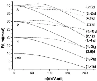
␯+ 1, where␯= 1 , 2 , 3 , . . . and the ground state is␯= 0. In the absence of the magnetic field 共B=0兲, the variation of the eigenenergy E共i,m兲, with the Rashba SOI parameter ␣, for

e0= 10 meV is shown in Fig. 1. When ␣ is zero, the two

coupled equations for spins up and down shown in Eq. 共2兲 are decoupled because of H±= 0 and H0± reduce to H0

⬘

共the Hamiltonian for the isotropic simple harmonic oscilla-tor兲 because B=0. Figure 1 shows that at ␣= 0 the ␯th excited state has ␯+ 1 doubly degenerate levels due to the

FIG. 1. Eigenenergy E共i,m兲 vs␣with B = 0 and e₀= 10 meV.

(5)

spins and each level has an oscillator energy of 共␯+ 1兲e0.

Each level of E共i,m兲 is labeled as 共i,m兲d or 共i,m兲u, where u and d are used to indicate the spin states up 共u兲 and down 共d兲. The spin up or down state is determined by examining the wave functions⌿1and⌿2in Eq.共2兲. A discussion of the

probability densities 共=⌿j *_⌿

j, j = 1 , 2兲 for the spins is

pre-sented later. The lowest 20 levels of E共i,m兲 are labeled as follows: for ␯= 0关共1,−1兲d,共1,0兲u兴; for ␯= 1关共1,1兲u, 共2,0兲d,共1,−2兲d,共2,−1兲u兴; for ␯= 2关共1,2兲u,共2,1兲d, 共3,−1兲d,共3,0兲u,共1,−3兲d,共2,−2兲u兴; for ␯= 3关共1,3兲u, 共2,2兲d,共3,1兲u,共4,0兲d,共3,−2兲d,共4,−1兲u,共1,−4兲d,共2,−3兲u兴. For ␣⬎0 all the energy levels are doubly degenerate for spins up and down; thus only the E共i,m兲’s with spin down 共i,m兲d are plotted in Fig. 1. The lowest energy level obtained from Eq.共9兲 is E共1,−1兲=9.969 86 meV, while E共1,−1兲 ap-proximated by Eq.共12兲 is 9.97 meV for␣= 10 meV nm. So long as B = 0 and ␣⬍15 meV nm, Eq. 共12兲 gives a good estimate for E共1,−1兲. With␣= 10 meV nm and e0= 10 meV, E共i,m兲 vs B is plotted in Fig. 2共a兲 for the lowest 20 levels.

When B = 0, there are ␯+ 1 doubly degenerate levels. When

B⬎0, all the degeneracies are lifted to yield 2共␯+ 1兲 levels

for ␯= 0 , 1 , 2 , 3 but the energy splittings are too small to be shown in Fig. 2共a兲. If we choose ␣= 50 meV nm and

e0= 10 meV, the E共i,m兲 vs B curves plotted in Fig. 2共b兲

show clearly that there are 20 different levels due to the

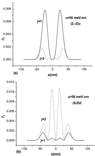
energy splitting. The probability densities are ␳j=兩⌿j兩2,

where j = 1 is for spin up and j = 2 is for spin down关see Eq. 共2兲兴 with␳1+␳2= 1. The probability densities as a function of x = r cos␪ with B = 1 T, e0= 10 meV and␣= 50 meV nm for

the eigenenergies E共2,−2兲 and E共4,0兲 are plotted in Figs. 3共a兲 and 3共b兲, respectively. In order to show both␳1and␳2,

␣ is intentionally chosen to be large. Figure 3共a兲 shows that

␳1 is the dominant component, and thus the共2,−2兲 state is

labeled with u 共spin up兲 with a polarization of P= +0.54, while Fig. 3共b兲 shows that ␳2 is the dominant component,

and thus the共4,0兲 state is labeled with d 共spin down兲 with a polarization of P = −0.49.

The energy splittings ⌬Ej as a function of B for

␣= 10 meV nm and e0= 10 meV are plotted in Fig. 4 with E共1,0兲−E共1,−1兲 labeled as ⌬E1, E共2,0兲−E共1,1兲 labeled as

⌬E2, and E共2,−1兲−E共1,−2兲 labeled as ⌬E3. Solid curves are

evaluated with g = −8 共including Zeeman splitting兲, while dashed curves are evaluated with g = 0 共excluding Zeeman splitting兲.

The energy splittings for the lowest two energy levels ⌬E1= E共1,0兲−E共1,−1兲 vs B for␣= 10, 30, 50 mev nm with e0= 10 meV are plotted in Fig. 4共a兲. Here we observe that

⌬E1 can be suppressed due to the Zeeman splitting with g = −8. Notice that⌬E1is small; even when B is 6 T,⌬E1is

FIG. 2. Eigenenergy E共i,m兲 vs B for e0= 10 meV with共a兲␣= 10 meV nm and共b兲␣= 50 meV nm.

FIG. 3. Probability densities ␳j共j=1,2兲 as a function of x with B=1 T,

␣= 50 meV nm, and e0= 10 meV for共a兲 the 共2,−1兲 state and 共b兲 the 共4,0兲 state. Solid curves for j = 1共spin up marked with u兲 and dotted curves for

j = 2共spin down marked with d兲.

(6)

only 0.05 meV. However,⌬E1can increase rapidly as␣

in-creases. Figure 4共b兲 shows that the energy splittings for the excited states⌬E2 and⌬E3 vs B. Both⌬E2 and⌬E3

calcu-lated with the Zeeman splitting differ significantly from⌬E2

and⌬E3calculated without the Zeeman splitting. The

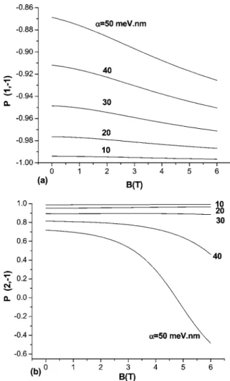
polar-ization P defined in Eq. 共10兲 versus B for ␣= 10, 30, 50 meV nm with e0= 10 meV is plotted in Fig. 5共a兲 for

the lowest state 共1,−1兲 and Fig. 5共b兲 for the excited state 共2,−1兲. Figure 5共a兲 shows that when␣is small the variation of P with B is negligible共⬇−0.99 spin down兲, but when␣is larger the variation of P with B becomes stronger. This rapid change in P with B is even more evident for the共2,−1兲 state as shown in Fig. 5共b兲. It is interesting to note that in Fig. 5共b兲 when B is larger than 4.8 T, the polarization P changes sign from positive to negative.

As an application of our numerical calculations for

E共i,m兲, we discuss how the Fermi energy Ef and the

mag-netization M of the quantum disk at 0 ° K vary with B for the case of e0= 10 meV with strong SOI␣= 50 meV nm for

vari-ous Ne’s. Let us assume that the total number of electrons in

the system is a constant, then Ne in Eq. 共13兲 indicates that Ef must vary with B in order to keep Neconstant. We use

30 E共i,m兲 levels to plot Fig. 6. Figure 6共a兲 shows that

共1兲 when Neis 2, Ef increases monotonically as B increases;

共2兲 when Ne is 4, Ef shows a small peak located at B⬇0.3 T because crossing occurs between the 关共2,0兲d and

共1,2兲d兴 states as depicted in Fig. 2共b兲; 共3兲 when Neis 6, Ef

shows two small peaks located at B⬇1.2 T and 1.65 T be-cause crossings occur between the 关共2,−1兲d and 共1,2兲d兴 states and between the关共2,−1兲u, 共2,1兲d兴 states, respectively, as depicted in Fig. 2共b兲; 共4兲 when Ne is 8, Ef shows three

small peaks located at B⬇0.3, 2.1, and 2.55 T. At 0 K, M in Eq. 共13兲 reduces to⳵Etot/⳵B, where Etotis the total electron

energy of the system. M as a function of B is plotted in Fig. 6共b兲 and shows oscillatory behavior. The more electrons in the disk, the more oscillations occur in M as a function of B. IV. CONCLUSION

We have calculated the electron energy levels for quan-tum disks with parabolic potential profiles in a magnetic field by solving a 2⫻2 single electron Hamiltonian for electron spins including the Rashba SOI. We showed that in the pres-ence of the spin-orbit interaction, the azimuthal quantum number m is no longer a good quantum number, and found that the doubly degenerate electron energy levels E共i,m兲 de-crease as ␣ increases and crossing occurs between energy levels. When the magnetic field B is turned on, the double degeneracy in the energy levels is removed, and the ␯th

FIG. 4. Energy splitting ⌬Ej as a function of B with e0= 10 meV for 共a兲 ⌬E1, ␣= 10, 30, and 50 meV nm, and for 共b兲 ⌬E2, ⌬E3 with

␣= 10 meV nm. Solid 共dotted兲 curves represent Zeeman splitting included 共excluded兲. 关⌬E1= E共1,0兲−E共1,−1兲, ⌬E2= E共2,0兲−E共1,1兲, and ⌬E3= E共2,−1兲−E共1,−2兲兴

FIG. 5. Polarization P as a function of B with e0= 10 meV and␣= 10, 20, 30, 40, and 50 meV nm for共a兲共1,−1兲 and 共b兲共2,−1兲 states.

(7)

excited state splits into 2共␯+ 1兲 levels. The spin states are determined by examining the wave functions for each corre-sponding eigenvalue E共i,m兲. The energy splitting ⌬Ej and

the polarization兩P兩 increase as␣and B increase. The Landé factor of the electron spin for InAs 共g=−8兲 can affect the value of ⌬Ej共B兲 significantly. The Fermi level versus B

shows oscillations because of the crossing behavior between states E共i,m兲’s. The magnetization versus B also shows os-cillatory behavior.

ACKNOWLEDGMENTS

One of the authors共W.C.C.兲 wishes to acknowledge the support by the National Science Council of the Republic of China under Contract No. NSC94-2112-M-009-013. Another author 共J.L.兲 would like to thank the support from the National Center for Theoretical Science during his visit to the Department of Electrophysics, National Chiao Tung University.

1_{A. Kuzmich and E. S. Polzik, Appl. Phys. Lett. 85, 5639}_共2000兲. 2_{A. Barenco, D. Deutch, and A. Ekert, Phys. Rev. Lett. 73, 4083}_共1995兲. 3_{D. P. DiVincenzo, Phys. Rev. A 51, 1015}_共1995兲.

4_{J.-P. Leburton, S. Nagaraja, P. Matagne, and R. M. Martin, Microelectron.} J. 34, 485共2003兲.

5_{J. H. Smet, R. A. Deutschmann, F. Ertl, W. Wegscheider, G. Abstreiter,} and K. von Klitzing, Nature共London兲 415, 281 共2002兲.

6_{E. I. Rashba, Fiz. Tverd. Tela} _{共Leningrad兲 2, 1224 共1960兲; 关Sov. Phys.} Solid State 2, 1109共1960兲兴; Y. A. Bychkov and E. I. Rashba, J. Phys. C

17, 6039共1984兲.

7_{J. C. Egues, G. Burkard, and D. Loss, Phys. Rev. Lett. 89, 176401}_共2002兲. 8_{E. I. Rashba and Al. L. Efros, Phys. Rev. Lett. 91, 126405}_共2003兲. 9_{J. Nitta, T. Akazaki, H. Takayanagin, and T. Enoki, Phys. Rev. Lett. 78,}

1335共1997兲.

10_{D. Grundler, Phys. Rev. Lett. 84, 6074}_共1999兲.

11_{F. E. Meijer, A. F. Morpurgo, T. M. Klapwijk, T. Koga, and J. Nitta, Phys.} Rev. B 70, 201307共2004兲.

12_{S. Datta and B. Das, Appl. Phys. Lett. 56, 885}_共1990兲. 13_{S. A. Tarasenko and N. S. Averkiev, JETP Lett. 75, 552}_共2002兲. 14_{X. F. Wang and P. Vasilopoulos, Phys. Rev. B 67, 085313}_共2003兲. 15_{G. Usaj and C. A. Balseiro, Phys. Rev. B 70, 041301R}_共2004兲. 16_{S. Debald and B. Kramer, Phys. Rev. B 71, 115322}_共2005兲. 17_{T. Chakraborty and P. Pietiläinen, Phys. Rev. B 71, 113305R}_共2005兲. 18_{P. Lucignano, B. Jouault, A. Tagliacozzo, and B. L. Altshuler, Phys. Rev.}

B 71, 121310R共2005兲.

19_{M. G. Pala, M. Governale, U. Zülicke, and G. Iannaccone, Phys. Rev. B}

71, 115306共2005兲.

20_{S. Bandyopadhyay and M. Cahay, Superlattices Microstruct. 32, 171} 共2002兲.

21_{W. H. Kuan, C. S. Tang, and W. Xu, J. Appl. Phys. 95, 6368}_共2004兲. 22_{T. Chakraborty and P. Pietläinen, Phys. Rev. B 71, 113305}_共2005兲. 23_{S. Debald and C. Emary, Phys. Rev. Lett. 94, 226803}_共2005兲. 24_{E. T. Jaynes and F. W. Cummings, Proc. IEEE 51, 89}_共1963兲.

25_{F. M. Hashimzade, A. M. Babayev, S. Cakmak, and S. Cakmaktepe,} Physica E共Amsterdam兲 25, 78 共2004兲.

26_{E. N. Bulgakov and A. F. Sadreev, JETP Lett. 73, 505}_共2001兲. 27_{S. Raymond et al., Phys. Rev. Lett. 92, 187402}_共2004兲. FIG. 6. 共a兲 The Fermi energy EF and 共b兲 magnetization M vs B for ␣

= 50 meV nm with e0= 10 meV.