Item 987654321/15186

全文

(1)中華民國國立成功大學資訊工程學系博士論文. 特徵對應之紋理貼圖技術 Texture Mapping on 3D Surface with Hard Constraints. 研究生：顏韶威. Student: Shao-Wei Yen. 指導教授：李同益博士. Advisor: Dr. Tong-Yee Lee. Department of Computer Science and Information Engineering, National Cheng Kung University, Tainan, Taiwan, R.O.C. Dissertation of Doctor of Philosophy June, 2009. 中華民國九十八年六月.

(2)

(3)

(4) 特徵對應之紋理貼圖技術作者：顏韶威. 指導教授：李同益教授. 中華民國國立成功大學資訊工程學系博士班. 摘要紋理貼圖是電腦繪圖上相當普遍的技術；藉由輸入的二維影像，紋理貼圖可以利用影像中豐富的資訊與細節來加以擬真三維網格模型。本論文包含了三個不同而有效的紋理貼圖演算法，這三個演算法的設計演進分別從無特徵對應的紋理貼圖技術至有特徵對應的紋理貼圖演算法。第一個演算法可應用於任意的三維表面，主要的目標是著重於無失真的貼圖座標計算，但不考慮使用者給定的特徵位置對應。為了於三維模型上進行紋理貼圖，我們提出了一個架構來參數化任意三維表面至二維平面上。我們的方法不需要固定的參數化邊界，而且貼圖座標可以利用線性稀疏矩陣系統來有效率的求得解答；所以這個系統的執行表現可以達到互動式的操作反應。第二個與第三個演算法為有特徵對應的紋理貼圖演算法。有特徵對應的紋理貼圖是一個在電腦圖學上重要而且相當具挑戰性的問題。第二個演算法的主要觀念是重複的切割參數化的平面，直到每個切割出來的子區域僅剩下一個特徵點為止。由於每個子區域只包含一個特徵點，所以特徵點的對齊問題已被大大的簡化，每個子區域只需單獨計算處理即可對齊所有的特徵點。在第三個特徵對應的紋理貼圖方法中，我們一開始於二維平面空間裡推導一個理論上強健地、無翻轉三角形的變形演算法；之後我們應用此變形方法到有特徵對應的紋. i.

(5) 理貼圖。這個演算法可以在視覺上擁有更好的繪圖呈現，而主要的關鍵在於本方法只需增加了少數的 Steiner vertices 在參數化後的三角網格模型上，即可滿足使用者的特徵對應需求。關鍵字: 紋理貼圖、參數化、貼圖變形量、聚集、虛擬點、翻轉、位置限制、變形、Steiner vertex. ii.

(6) Texture Mapping on 3D Surface with Hard Constraints Student: Shao-Wei Yen. Advisor: Dr. Tong-Yee Lee. Department of Computer Science and Information Engineering National Cheng Kung University, Tainan, Taiwan, R.O.C.. Abstract Texture mapping is a common and very useful technique in computer graphics. Texture mapping adds the detailed information of the user-specified image to the 3D models and represents the rendering result more vividly and realistically. This thesis contains three efficient algorithms from texture mapping on 3D surface without positional constraints to texture mapping with hard positional constraints. The first one is to achieve distortion-free texture mapping on arbitrary 3D surfaces without constraints. To texture 3D models, we propose a scheme to flatten 3D surfaces into a 2D parametric domain. Our method does not require the two-dimensional boundary of flattened surfaces to be stationary. The first parameterization scheme can be efficiently realized by a linear sparse matrix system and yields interactive performance. The second and third algorithms are texture mapping with hard positional constraints. Texture mapping with positional constraints is an important and challenging problem in computer graphics. The idea of second one is to partition the parametric map until each sub-region contains one feature points. Then we can easily handle each sub-region and complete the alignment of all feature points. In the third algorithm, we first present a theoretically robust, foldover-free 2D mesh. iii.

(7) warping algorithm. Then we apply this warping algorithm to texture mapping on 3D triangle meshes with hard positional constraints. The third algorithm can generate more pleasing visual representation, add fewer Steiner vertices on the 3D mesh embedding domain, and satisfy all user-specified constraints without foldovers. Keywords: texture mapping, parameterization, texture stretch, clustering, virtual points, foldover, positional constraints, warping, Steiner vertex. iv.

(8) Acknowledgements I sincerely thank to my advisor Tong-Yee Lee. His advice and guidance are constructive, his insightful suggestion and enthusiastic attitude inspire my positive interest in the field of computer graphics. I also thank to Prof. Yung-Nien Sun, his leadership and knowledge guide the visual system laboratory keep progressing. And thanks to all the members in the visual system laboratory NCKU. Finally, I sincerely give my gratitude to my family and my girlfriend, their support are invaluable.. v.

(9) Contents Chapter 1 Introduction .......................................................................................................... 1 1.1 Background and Objectives .................................................................................... 1 1.2 Contribution ............................................................................................................ 4 1.3 Organization ............................................................................................................ 5 Chapter 2 Related Work ........................................................................................................ 7 2.1 Parameterization without Constraints ..................................................................... 7 2.2 Parameterization with Constraints ........................................................................ 10 Chapter 3 General Texture Mapping on 3D Surfaces without Positional Constraints........ 13 3.1 Overview ............................................................................................................... 13 3.2 Methodology ......................................................................................................... 14 3.2.1 The Initial Setup ......................................................................................... 15 3.2.2 Reducing Distortion Using Clustering and Cutting ................................... 16 3.2.3 Virtual Points.............................................................................................. 20 3.2.4 Smoothing .................................................................................................. 22 3.3 Experimental Results............................................................................................. 23 Chapter 4 Constrained Texture Mapping using Partition Scheme ...................................... 28 4.1 Overview ............................................................................................................... 28. vi.

(10) 4.2 Parameterization with feature points..................................................................... 28 4.2.1 Initial parameterization .............................................................................. 29 4.2.2 Feature matching using a partitioning approach ........................................ 30 4.2.3 UV optimization ......................................................................................... 32 4.3 Results ................................................................................................................... 32 Chapter 5 Constrained Texture Mapping using Warping Scheme ...................................... 34 5.1 Overview ............................................................................................................... 34 5.2 Foldover-free 2D Triangle Mesh Warping ............................................................ 34 5.2.1 Definitions.................................................................................................. 35 5.2.2 Theoretical Analysis and Algorithm........................................................... 37 5.3 Texture Mapping with Hard Constraints ............................................................... 45 5.3.1 Overview and Definitions .......................................................................... 45 5.3.2 Constructing a Base Mesh.......................................................................... 47 5.3.3 Warping a Base Mesh................................................................................. 49 5.3.4 Smoothing the Embedding ......................................................................... 50 5.4 Experimental Results and Discussion ................................................................... 51 5.4.1 Results ........................................................................................................ 51 5.4.2 Discussion with Related Work ................................................................... 57 Chapter 6 Conclusion and Future Work .............................................................................. 60 vii.

(11) 6.1 Conclusion............................................................................................................. 60 6.2 Future Work........................................................................................................... 61 References ........................................................................................................................... 63 Vita ...................................................................................................................................... 69. viii.

(12) List of Tables Table 1: Comparison between cutting method and Gu et al. [13]....................... 27 Table 2: Mean texture stretch ratio statistics for five examples .......................... 27 Table 3. The statistics for the texture mapping samples. #Steiner (initial) and #Steiner (final) are the number of Steiner vertices before and after removing. ..................................................................................................................... 59. ix.

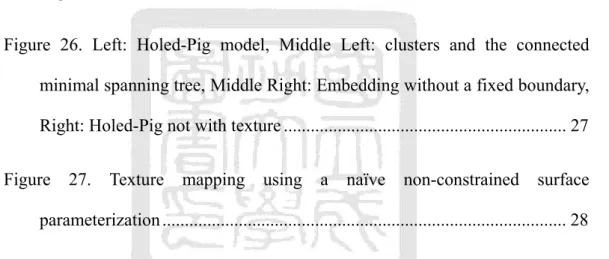
(13) List of Figures Figure 1. Left: Ball model, Middle Left: clusters and the connected minimal spanning tree, Middle Right: Embedding without a fixed boundary, Right: Ball with texture ............................................................................................ 2 Figure 2. Left: Knot model, Middle Left: clusters and the connected minimal spanning tree, Middle Right: Embedding without a fixed boundary, Right: Knot with texture........................................................................................... 2 Figure 3. Left: a 3D model, Middle: texture mapping without constraints, Right: texture mapping with constraints .................................................................. 3 Figure 4. Texture mapping with positional constraints using warping scheme .... 4 Figure 5. Mean value coordinates [8].................................................................... 7 Figure 6. Remeshing a triangle mesh (a) using barycentric (b), discrete harmonic (c), and mean value (d) (M. S. Floater and K. Hormann [9]) ....................... 8 Figure 7. Linear angle based parameterization [47].............................................. 9 Figure 8. The texture atlas and the mapping result from [23]............................. 10 Figure 9. A challenge case that [18] can not handle.............................................11 Figure 10. Inter-surface mapping of [33] ............................................................ 12 Figure 11. The results of (a) TextureMontage [48] and (b) FlexiStickers [41] ... 12 Figure 12. Flow chart of the proposed scheme ................................................... 15 Figure 13. (a): a torus model with one cut set (b): connected cut sets (c):. x.

(14) unconnected cut set ..................................................................................... 16 Figure 14. A bunny Model and its clustering result (solid white points are the center of the clusters) .................................................................................. 19 Figure 15. The vertices of outside circle is virtual points ................................... 21 Figure 16. The line is between a boundary vertex and the center of the embedding ................................................................................................... 21 Figure 17. Left: texture mapping without smoothing. Right: texture mapping with smoothing............................................................................................ 22 Figure 18. Left: a grid map of bounded square, Right: smoothing results of grid map .............................................................................................................. 22 Figure 19. Left: Rabbit model, Middle Left: clusters and the connected minimal spanning tree, Middle Right: Embedding without a fixed boundary, Right: Rabbit with texture ...................................................................................... 24 Figure 20. Left: Pig model, Middle Left: clusters and the connected minimal spanning tree, Middle right: Embedding without a fixed boundary, Right: Pig with texture ........................................................................................... 25 Figure 21. Left: Dinosaur model, Middle Left: clusters and the connected minimal spanning tree, Middle Right: Embedding without a fixed boundary, Right: Dinosaur with texture ....................................................................... 25 Figure 22. Left: Head model, Middle Left: clusters and the connected minimal spanning tree, Middle Right: Embedding without a fixed boundary, Right: Head with texture ........................................................................................ 25 xi.

(15) Figure 23. Left: Ball model, Middle Left: clusters and the connected minimal spanning tree, Middle Right: Embedding without a fixed boundary, Right: Ball with texture .......................................................................................... 26 Figure 24. Left: Knot model, Middle Left: clusters and the connected minimal spanning tree, Middle Right: Embedding without a fixed boundary, Right: Knot with texture......................................................................................... 26 Figure 25. Left: Two-holes model, Middle Left: clusters and the connected minimal spanning tree, Middle Right: Embedding without a fixed boundary, Right: Two-holes with texture..................................................................... 26 Figure 26. Left: Holed-Pig model, Middle Left: clusters and the connected minimal spanning tree, Middle Right: Embedding without a fixed boundary, Right: Holed-Pig not with texture ............................................................... 27 Figure. 27.. Texture. mapping. using. a. naïve. non-constrained. surface. parameterization .......................................................................................... 28 Figure 28. vj is the one-ring neighbor of vi for triangulation mesh...................... 29 Figure 29. (a) and (b): feature correspondence between a 3D model and a texture image; (c) and (d): the uv map of the mean value coordinates with and without virtual boundary ............................................................................. 29 Figure 30. Each partitioning step determines two separate groups of features in texture and uv domains ............................................................................... 30 Figure 31. The alignment of single feature f ....................................................... 31 Figure 32. Finding a partitioning path in u,v domain.......................................... 32 xii.

(16) Figure 33. The smoothing of uv map. (a) original texture (b) smoothed with a harmonic map (c) smoothed with L2 stretch metric ................................... 33 Figure 34. Texuring a man head with a bear image ............................................ 33 Figure 35. Texturing a monkey face with a lion image....................................... 33 Figure 36. P(v ) : the union of triangles adjacent to v , ∂P(v ) : the boundary of P(v ) , and Q (e) : the enclosing quadrilateral of e . ................................ 36 Figure 37. ∂P(v ) consists of red edges. When v moves to vα , each shaded triangle becomes degenerated, i.e., folded over........................................................ 36 Figure 38. (a) Eα(v) = {e}. When v moves to the open interval ( pi , vα ) ,. Q (e) becomes convex and e (i.e., p1 p 3 ) can be swapped. (b) edge e is swapped and v moves to vα ......................................................................... 38 Figure 39. (a) ∠p1 p 2 p 3 > π in Q( vp 2 ). (b) ∠p 3 vp1 ≥ π in Q( vp 2 ). (c) vp 2 is swapped and v moves to vα . ....................................................................... 39 Figure 40. Shaded triangles are degenerated when v moves to vα . (a) Eα(v) = { q 2 q 3 , q3 q 4 , q7 q8 }. The connected components of Eα(v) are C1 = { q 2 q 3 , q3 q 4 } and C2 = { q7 q8 }. Before v moves to vα , we can swap vq4 to remove Δvq 3 q 4 as shown in (b) and then swap vq3 to remove Δvq 2 q 3 as shown in (c)................................................................................................. 39 Figure 41. (a) vα is on a vertex u of Eα(v). u can find a direction um′ in (b). Then u can move to the interval (u, uα′ ) and v can move to vα in (c). ................... 41 Figure 42. (a)-(b) input triangle mesh M and 2D texture. (c) the planar embedding of M with virtual boundary. (d)-(f) warping algorithm is used to align xiii.

(17) constraints. (g) the resulting embedding is further smoothed. (h) Resulting textured model............................................................................................. 46 Figure 43. fi are feature vertices and red dotted lines are edges of G. A corresponding path (green) of f 3 f 4 was computed in (b). In (a) and (b), an edge v1v 2 of PM+ divides the enclosing boundary of f 1 f 3 into two sub-regions. A Steiner vertex (blue) is added and the corresponding path of f 1 f 3 is shown in light blue......................................................................... 47 Figure 44. mesh smoothing using (a) [18], (b) the metric φ (t ) , and (c) the weighted metric w ⋅ φ (t ) ............................................................................................. 50 Figure 45. Example of failure in Zöckler et al. [50]. The red nodes are feature vertices and the black nodes are the other mesh vertices encoded by the barycentric coordinates. The shaded triangle is flipped when the feature f1 continues moving ........................................................................................ 52 Figure 46. (a) feature vertex C is at the different side of path AB (b) path AB does not prevent C from moving since it can be swapped. (c) feature matching from (b). (d) the matching paths using [18]. (e) feature matching from (d). Note that the vertices inside each triangle patch are not shown in (b)-(e) for easy illustration. .......................................................................................... 53 Figure 47. (a) input mesh M. (b) input texture. (c) the embedding PM+ of M. (d) the initial paths(green) of base mesh BM+. (e) BM+ after feature matching. (f) texture mapping result after smoothing from (e). (g) the path matching using [18]. (h) texture mapping result of [18]....................................................... 53 Figure 48. (a) input mesh M. (b) input texture. (c) the embedding PM+ of M and the xiv.

(18) initial paths(green) of base mesh BM+. (d) initial base mesh BM+. (e) BM+ after feature matching. (f) texture mapping result after smoothing from (e). (g) the path matching using [18]. (h) texture mapping result of [18]. .................... 54 Figure 49. (a) input mesh M. (b) input texture. (c) the embedding PM+ of M and the initial paths(green) of base mesh BM+. (d) initial base mesh BM+. (e) BM+ after feature matching. (f) texture mapping result after smoothing from (e). (g) the path matching using [18]. (h) texture mapping result of [18]. .................... 55 Figure 50. More results. In (c) and (d), the embeddings are the final results after smoothing. ................................................................................................... 56 Figure 51. (a) a hairless head model with the texture image. (b) texture mapping results. (c) initial parametric map. (d) final embedding after mesh smoothing. ..................................................................................................................... 57 Figure 52. An Igea model and the texture mapping results................................. 59. xv.

(19) Chapter 1 Introduction 1.1. Background and Objectives. Texture mapping is one of the most important and common techniques in computer graphics. It brings rich information like color, normal, and surface displacement to enhance the reality of computer-generated 3D models by gluing a 2D image to the polygon surface. Texture mapping usually involves the computation of (u, v) texture coordinates. And the mesh planar parameterization is the most common way to determine the texture coordinates. The parameterization is basically a flattening process of a 3D disk-like surface. The assignment of texture coordinates from a good parameterization usually produces pleasure visual representation while a 2D image is texturing to the 3D model. And good parameterization also has low distortion. The distortion can have the variety of measurements such as angle, area, and length ratio between the 3D model and the parametric domain. In this thesis, we propose three different algorithms for the texture mapping on 3D models. They involves texture mapping without and with positional constraints in the following: First, we develop a system approach for texture mapping a 3D model without constraints and with low distortion. Generally, parameterization of a 3D surface usually has high distortion at the location of high curvature. To solve this issue, a clustering algorithm is introduced. The clustering method gathers the locations with high distortion from the 2D parametric domain. We connect these locations to form a cutting path that cuts the 3D model along high distortion edges. To further improve the quality of parameterization, we also propose a parameterization with free boundary by adding virtual points outside the. 1.

(20) original embedding in the parametric domain. At the final stage of this approach, we use the inverse warping of the 2D texture image to produce final optimal texture coordinates.. Figure 1. Left: Ball model, Middle Left: clusters and the connected minimal spanning tree, Middle Right: Embedding without a fixed boundary, Right: Ball with texture. Figure 2. Left: Knot model, Middle Left: clusters and the connected minimal spanning tree, Middle Right: Embedding without a fixed boundary, Right: Knot with texture Most of parameterization methods [5], [7], [8], [13], [14], [21], [26], [28], [29], [30], [32], [34], [36], [38], and [49] generate texture coordinates without positional constraints. Without constraints, the texture mapping of a 3D model with a specific texture image may sometimes look very strange as shown in Figure 3.. 2.

(21) Figure 3. Left: a 3D model, Middle: texture mapping without constraints, Right: texture mapping with constraints The second and the third algorithms of this thesis are about the texture mapping with hard constraints. That means some vertices of the 3D model should exactly satisfy the positional constraints on the parametric domain. The difficulty of this problem is the parameterization should satisfy the constraints with no foldovers and should not distort the parametric map too much while the constraints are assured. There are two approaches for texture mapping with constraints in this thesis. In the second algorithm, we consider the parameterization with positional constraints. The main concept of this approach is to partition the convex parametric domain until each sub-region contains only one feature point. After each sub-region is constructed, the target position of each feature point is also inside the correspondent sub-region. Then we can easily align each feature point by partitioning each sub-region into four triangle patches. This approach is foldover free and satisfies hard constraints. In the third algorithm, we first develop a warping algorithm without foldovers. The design of the proposed warping algorithm is based on a set of theoretical analysis, and the basic idea behind it is to avoid foldovers by the edge swap operators. Then we apply it to texture mapping with positional constraints. It is important that we uses path swap instead 3.

(22) of edge swap to avoid damaging the original connectivity of the 3D model. We also design a better stretch metric for measurement of parametric distortion. Our stretch metric has better visual perception than the state of the art texture mapping algorithm [18].. Figure 4. Texture mapping with positional constraints using warping scheme. 1.2. Contribution. This thesis contains three texture mapping algorithms. The first one is texture mapping using clustering method and has the following contributions: •. This method can flatten 3D surfaces efficiently without the fixed boundary on 2D parametric domain. Thus we present a faster and a lower texture stretch scheme for texture mapping on 3D surface.. •. To reduce texture stretch, we propose a clustering strategy to find a cutting path. We also apply virtual points and smoothing for further reduction of texture stretch. All stages of our algorithm can be realized efficiently to reach an interactive runtime performance.. •. In addition, the proposed method can handle both genus-0 and non-genus-0 models by providing an interactive cutting approach. The second and third approaches are about texture mapping with hard constraints. The. 4.

(23) contributions of the second one can be summarized as follows: •. The feature matching idea of this algorithm is a divide-and-conquer strategy. It mainly based on the recursive partitioning procedure in the parametric domain. Such strategy simplifies the feature alignment problem since each sub-region of partition contains only one feature point.. •. We develop a path-finding method to build a cutting path to cut the parametric map into two disjoint regions. We can then iteratively partition the parametric map by stretching the cutting path at each division. And the third approach creates a new warping scheme by edge swap operators to satisfy. the user-specified positional constraints. The contributions and novelty can be described as follows: •. For a given 2D mesh, we propose a theoretically robust and foldover-free warping algorithm to match the positional constraints.. •. We extend this new warping algorithm to handle texture mapping with hard constraints. This new constrained texture mapping can handle more challenging constraints with less danger of distortions. Furthermore, our method adds a fewer number of Steiner vertices on the 3D mesh embedding.. 1.3. Organization. The rest of this thesis is organized as the following. Chapter 2 discusses the related works from general parameterization without constraints to parameterization with positional constraints. Chapter 3 discusses texture mapping without hard constraints using the. 5.

(24) clustering-based cutting paths. Using this system, we can apply texture mapping to any model with low distortion. And the run-time of computation is also efficient. In Chapter 4, an algorithm about texture mapping with hard constraints is proposed. We use the idea by partitioning the parametric domain to satisfy the user-defined constraints. And in Chapter 5, a novel and robust warping scheme is proposed. We then apply it to the texture mapping with hard constraints. We also demonstrate some challenge examples to illustrate the robust property of this algorithm. Then we conclude the proposed algorithms in this thesis in Chapter 6.. 6.

(25) Chapter 2 Related Work 2.1. Parameterization without Constraints. There have been many texture mapping methods proposed [7], [13], [14], [26], [29], [38], and [49]. Most of them discuss the issue of surface parameterization. In general, the topology of 3D surface meshes are usually required to be the same with a disk, because the connectivity of 3D surface meshes will have no changes and can be mapped to a plane during the surface parameterization process. Tutte [40] introduces the barycentric map which guarantees the existence of a one-to-one mapping, i.e., foldover free, for parameterizing a model into the (u, v) domain. Maillot et al. [26] group the facets of the input mesh by their normals and attempt to reduce distortion by minimizing a norm of the Green-Lagrange deformation tensor. They also design an interactive tool to allow user to edit the atlases in the texture space. Eck et al. [5] minimize the harmonic energy to approximate the harmonic map and this method can be solved efficiently by a linear sparse matrix. Floater [8] develops the mean value coordinates to mimic the discrete harmonic map and this mapping is bijective.. Figure 5. Mean value coordinates [8]. 7.

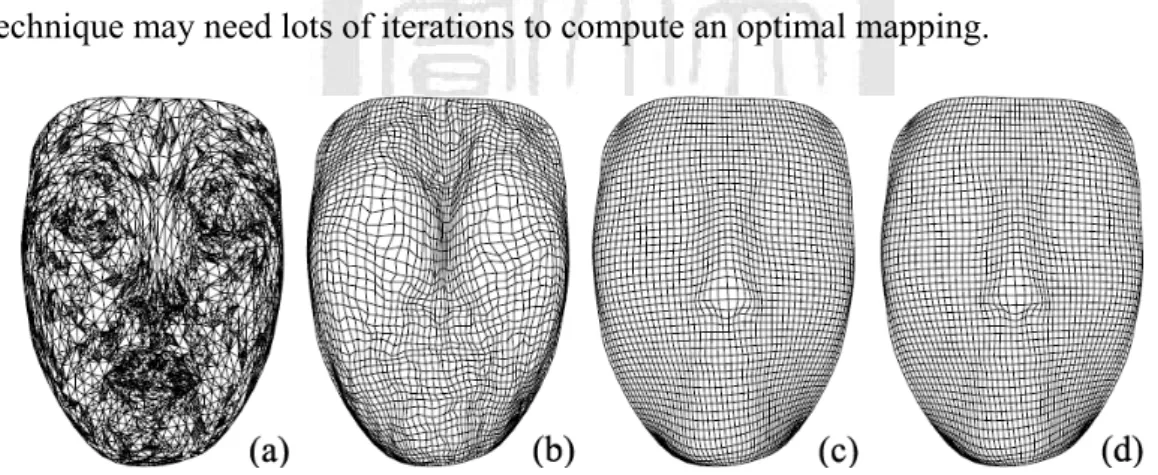
(26) [5] and [8] can be realized efficiently by solving a linear system, however, the boundary vertices are required to be on a convex 2D polygon. In [8], the convex boundary guarantees the property of bijective. Hormann and Greiner [14] derive a formula that measures the distortion of the parameterization and is also invariant for affine transformation. This method does not require the boundary vertices to be fixed on the convex 2D polygon. However, the optimization of solution is slow due to the non-linear mathematical property. Sander et al. [32] define a texture stretch metric for surface parameterization. Their texture stretch measures the local scale including the maximum and minimum stretch for each triangle face. This approach uses a relaxation approach similar to MIPS [14] to iteratively flatten 3D surfaces since the formula of the texture stretch is nonlinear. Their texture stretch metric produces better results than those of several previous methods [5], [14], and [26]. However, this technique may need lots of iterations to compute an optimal mapping.. Figure 6. Remeshing a triangle mesh (a) using barycentric (b), discrete harmonic (c), and mean value (d) (M. S. Floater and K. Hormann [9]) Sorkine et al. [38] introduce a bounded-distortion parameterization to guarantee that each triangle's distortion will strictly be below a user-defined threshold. This method does not need to map the surface into a convex region and automatically maps the boundary to the plane. For complicated 3D models, it would create many patches such that more 8.

(27) discontinuous arise in texture mapping results. Sheffer and Sturler [35] explicitly consider the angle of the triangle mesh for the parameterization in the 2D domain. This approach does not require the boundary to be fixed in the 2D domain. The solution should be realized by a constrained optimization since the formulas are nonlinear. Zayer et al. [47] simplify the nonlinear equation of [35] by the logarithm modification. Then the solution can be computed efficiently by the least square minimization.. Figure 7. Linear angle based parameterization [47] Zigelman et al. [49] map the 3D surface to a plane using a multi-dimensional scaling method that tries to preserve the geodesic distance criterion. This method does not ensure no self-intersection between the triangles and the computation cost is expensive because of the geodesic distance calculations. Lévy et al. [23] approximate the conformal maps in least square sense. This mapping approach does not need to fix boundary and the computation can be performed efficiently. However this approach may generate folded-over triangles after parameterization.. 9.

(28) Figure 8. The texture atlas and the mapping result from [23]. 2.2. Parameterization with Constraints. Several methods [2], [3], [6], [17], [18], [22], [24], [31], [33], [36], and [48] have addressed the problem of parameterization under constraints, and several applications are explored including morphing, compatible parameterization, remeshing, and constrained texture mapping. Desbrun et al. [3] and Lévy [22] solve constraints using Lagrange multipliers and a least square system, respectively. However, both methods do not guarantee the bijective embedding. On the other hand, Lee et al. [20] use RBF to warp embedding for aligning features. However, this method may also create foldovers. Eckstein et al. [6] use a constrained simplification to align the constraints and reconstruct simplified vertices without foldovers by adding Steiner vertices. Fujimura et al. [10] present a 2D image warping method with several constraints. Their approaches repeatedly use the Delaunay triangulation and edge swaps to avoid foldovers. The examples presented in [6] and [10] are simple, so it is not clear how these methods are able to handle more complicated constraints. In addition, Zöckler et al. [50] also use [10] to handle feature constraints in 3D morphing. However, the authors mention that this approach can potentially create foldovers. 10.

(29) when the positions of the corresponding features are very distinct between the source and the target embeddings. Kraevoy et al. [18] describe a state-of-the-art matchmaker algorithm for solving constraints in texture mapping. However, this algorithm may fail because it does not consider consistent neighbor ordering as mentioned in [33].. Figure 9. A challenge case that [18] can not handle Many methods for surface parameterization with constraints have been introduced to embed a 3D surface onto a simpler intermediate domain. Alexa [2] suggests a computationally intensive, relaxation-based approach to align feature vertices between two spherical parameterizations. This algorithm can potentially fail for a large number of features. Later, Lin et al. [25] use edge swaps to solve this problem on spherical embeddings. However, the edge swaps can damage the geometric surface. Praun et al. [31] consistently parameterize a set of genus-0 meshes into a user-specified simplicial complex. However, this approach potentially produces swirling paths, thereby increasing the distortion. Later, Schreiner et al. [33] and Kraevoy et al. [17] extend [18] and [31] to consistently parameterize models with the same genus. Recently, Lee et al. [19] propose a method to consistently parameterize models with different genus on the spherical domain. In this method, the CSG operation potentially damages the surface, in particular, for areas near holes.. 11.

(30) Figure 10. Inter-surface mapping of [33] Zhou et al. [48] build a mesh texturing framework to edit the texture coordinates with several input 2D images. They also develop the texture inpainting technique to fill the mesh triangles without texture coordinates. The inpainting method basically can be realized by solving the Poisson equation.. (a). (b). Figure 11. The results of (a) TextureMontage [48] and (b) FlexiStickers [41] Tzur and Tal [41] consider the photography effects for the texture mapping with positional constraints. This approach estimates the local camera parameter at each mesh vertex and computes the texture coordinates by the optimization of all camera parameters.. 12.

(31) Chapter 3 General Texture Mapping on 3D Surfaces without Positional Constraints 3.1. Overview. Texture mapping is one of the most important techniques in computer graphics. It can enhance the reality of computer-generated 3D models. The most common way to texture 3D surfaces is to map the surface into an isomorphic planar representation. This operation is called surface parameterization or surface flattening. This planar representation is called embedding. Except for simple surfaces, such as cylinders, the surface parameterization always creates surface distortions in the 2D parametric domain. If we directly apply this 2D parameterization to the texture mapping, the texture image mapped onto a 3D surface is also distorted. It is a well-known differential geometry theorem that no isometric parameterization is in the plane for a general surface patch [1]. Hence, there is no easy way to parameterize a general 3D surface over a 2D domain without introducing distortion. In this chapter, the proposed method attempts to minimize the distortion in surface parameterization and to produce a distortion-free texture mapping on arbitrary 3D surfaces. Among the previous works, the proposed scheme of this chapter is most related to [13] and [29]. Piponi et al. [29] cut the closed surface and then use the cut seams as the boundaries for parameterization. They also blend the seams to reduce the discontinuity effect. This method may need lots of user-interactions to define the boundaries to the 2D plane. In contrast to [29], our proposed method would avoid iterations using a standard numerical method to quickly solve the linear system. Gu et al. [13] propose a method for cutting through high distortion area in the parametric domain. They use an iteration. 13.

(32) procedure that finds only one path to cut at a time until the distortion is below some prescribed threshold value. In contrast to this method, our method can cut over all high distortion regions at the same time using a clustering strategy. In addition, there have been many clustering approaches proposed in computer graphics research. Kalvin and Taylor [15] merge faces into face clusters to achieve the mesh simplification. Willmott et al. [45] propose a hierarchical face-clustering algorithm that provides an efficient radiosity simulation. Sander et al. [32] apply the merge operation to partition meshes into charts to their progressive mesh parameterization.. 3.2. Methodology. Generally, parameterization techniques can be classified into two types: 1) fixed boundaries in the parametric domain and 2) non-fixed boundaries. The methods with fixed boundaries often produce large distortions because the boundary shapes of the original 3D models are very different from those of their flattened surfaces in the 2D domain. However, the methods without fixed boundary as mentioned in section 3.1 often need costly computation to get the final embedding. Therefore, the main contribution of this framework can be summarized in the following. 1.. The proposed method can flatten 3D surfaces efficiently without the fixed boundary on 2D parametric domain. Thus we present a faster and a lower texture stretch scheme for texture mapping on 3D surface.. 2.. To reduce texture stretch, we propose a clustering strategy to find a cutting path. We also apply virtual points and smoothing for further reduction of texture stretch. All stages of our algorithm can be realized efficiently to reach an interactive performance.. 14.

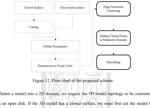
(33) 3.2.1. The Initial Setup. Figure 12 is the flow chart of the proposed scheme. We will explain in detail for the last three steps in later sections.. Figure 12. Flow chart of the proposed scheme To flatten a model into a 2D domain, we require the 3D model topology to be consistent with an open disk. If the 3D model has a closed surface, we must first cut the model to make the topology equivalent to an open disk. The user can interactively perform the cut procedure in our system. For models with genus greater than 1, we use some guide rules to cut all of them to a disk-like surface described as follows. For a torus with genus 1, which has one hole, a valid cut exists and consists of two closed paths like Figure 13(a). The two cut paths form the primitive cut set Cset for one 1 2 hole. For a model with genus 2 like Figure 13(b), we need two cut sets Cset and C set to. cut the surface. Once the two cut sets do not connect to each other, we add a path with no self-intersection to link the two sets. The surface with genus 2 can then be cut to a topological disk (see Figure 13(c)). By applying the same rule, a model with genus g must 15.

(34) 1 2 g first find g primitive cut sets Cset , C set ,..., C set and then paths are added to link all of them.. 1 Cset. 2 Cset. 2 Cset. 1 Cset. Figure 13. (a): a torus model with one cut set (b): connected cut sets (c): unconnected cut set After cutting a 3D model to a disk-like surface, we utilize a relaxation-based scheme from our previous work [20] to parameterize the 3D model into a 2D circular embedding. This surface parameterization can be solved using a sparse linear system. The relaxation equation is shown in (1). To simulate a spring-mass system we select w as the inverse of the edge length in 3D. Later in Section 3.2.3, we will explain the choice of the spring-mass system.. ∑ (w p ) = (1 − λ ) p + λ ∑ w ki. ' i. p. j =1 ki. i. j =1. j. j. (1). j. Where w: weight, λ: the speed of relaxation, and pj: 1-ring neighboring vertices of pi. 3.2.2. Reducing Distortion Using Clustering and Cutting. After the surface is parameterized into a circular embedding using the relaxation-based scheme, we usually find many vertices clustered in some areas of the embedding. These clustered areas are very possible to have higher parametric distortions. Gu et al. [13]. 16.

(35) suggest using cutting to reduce the distortion. Their parameterization approach iteratively finds regions of maximal distortion and connects the regions to the boundary using a path. However, this is very computationally expensive to repetitively execute parameterization and find each region with maximal distortion. In contrast, the proposed method does not require repetitive surface parameterization. We propose a clustering algorithm to find a cutting path going through the distorted areas. We then connect the cutting path to the boundary, cut the model and then execute the surface parameterization. Our clustering scheme is described in the following:. Clustering Algorithm 1.. Determine the vertices that would be joined to the computation of clustering algorithm. In our implementation, we calculate texture stretch L [32] of all vertices. If its texture stretch value is larger than the mean of all vertices, it would be added into a queue for clustering calculation. The texture stretch L can be defined in the following equation:. L(T ) =. (Γ. 2. + γ 2 )/ 2. Where Γ and γ represent the largest and smallest scale value while mapping a unit length from parametric domain to 3D surface domain, and T is a triangle of the mesh. 2.. Define a Guassian function GR that indicates the effective region of a cluster. GR (C − Pi ) = e. − C − Pi. C: vertex uv position on the parametric domain Pi: the position of i-th cluster's center. 17. 2. / R2.

(36) R: the cluster radius 3.. Initialize the first cluster. We choose the vertex with the maximum texture stretch value to be the center of the first cluster.. 4.. Calculate the centers of the other clusters new = arg j max( N (C j ; P1 ,..., PM , j = 1...n )) if N (C new ; P1 ,..., PM ) ≥ ε then PM +1 ← C new. Pi: clusters which have already been determined Cj: (u, v) position of the vertex j. ε: defined value for the termination of repeat loop The definition of function N is below: N (C j ; P1 ,..., PM ) = ∏k =1 [1 − GR (C − Pk )] M. Where the N function can be thought as the probability that vertex Cj is not belonging to other clusters P1,...,PM. From the above procedure, we determine all cluster centers. For each loop, the proposed clustering algorithm will determine the vertex that is the most irrelevant to the other clusters. If the function N value is less than the user-defined threshold ε, the clustering procedure would be terminated. Figure 14 shows an example of clustering and three centers are found.. 18.

(37) Figure 14. A bunny Model and its clustering result (solid white points are the center of the clusters). Minimal Spanning Tree Cutting After executing clustering algorithm, we need to get a path to connect all clusters and connect this path to the boundary in the embedding. For this purpose, we find a tree to connect these cluster centers. In our implementation, we adopt the standard Kruskal's minimal spanning tree algorithm. To assign the weight of a graph edge, we combine both the edge length and the texture stretch together. We attempt to find a minimal spanning tree that is over high distortion areas and has the minimal path length. The cutting path is founded using the following steps: 1.. For each pair of clusters, we compute the shortest path. The edge weight is set using the following equation. Edge Weight = 3D length + 1/(texture stretch). 2.. We then obtain a complete graph for connecting all clusters.. 3.. Calculate the minimal spanning tree of this complete graph.. 19.

(38) 3.2.3. Virtual Points. Once the cutting path is found, we cut the model and re-parameterize the model to a circular embedding again. At this stage, the boundary of the embedding is still fixed. In this section, we will add virtual points to pull the boundary of this circular embedding and to adaptively modify the boundary for reducing distortion. The circular embedding in our system is a simulation of the spring-mass system. Each edge of a 3D model is placed with a spring. The potential energy of a spring is equal to. E=. 1 2 Kx . K is the spring constant and x is the length of the spring. In our setup, K is 2. equal to the inverse of its corresponding 3D edge length. Then the total energy of the whole mesh is Etotal =. 1 K ij ( f (vi ) − f ( v j )) 2 2 ( vi ,v j )∈Edge. ∑. (2). , where f(v) is the uv position in the 2D parametric domain. If the system reaches stable equilibrium, the total energy Etatal would be minimized. Then the minimization of the total energy can be realized using a linear system [12]. In the outside of the circular embedding, for each boundary vertex, we put a corresponding vertex called virtual point along the direction from the center of the circle to the boundary vertex. See an example in Figure 15. We add a virtual spring between a boundary vertex and a virtual point. The spring constant of each virtual point is in the proportion to the inverse of the 3D length the distance of the shortest path from a boundary vertex to the center. The virtual springs then pull each boundary vertex outward. With adding these extra virtual points, we have the flexibility to re-define the boundary positions and can potentially reduce the distortion of parameterization. 20.

(39) For calculating the spring constants of boundaries, we may directly apply the Dijkstra's single source shortest path algorithm to compute the 3D surface length. Because the path computation is limited on triangle edges, this method may not always produce good and smooth results (Figure 16: left). For this problem, we can subdivide the 3D mesh to increase the accuracy of the 3D path length, but it is computationally expensive. Alternatively, we find each path directly from the embedding by a line connects the center to each boundary vertex (see an example in Figure 16: right). We then find line intersections and compute their corresponding 3D positions. In this manner, we can obtain an approximately shortest path in 3D. Finally, similar to [20], we can organize this spring-based system as a sparse linear system and we can solve it efficiently.. Figure 15. The vertices of outside circle is virtual points. Figure 16. The line is between a boundary vertex and the center of the embedding. 21.

(40) 3.2.4. Smoothing. Smoothing is the last step of our procedure. The main smoothing concept involves warping the texture used for texture mapping. The mapping distortion can then be further improved. Figure 17 illustrates the effects of smoothing for texture mapping. In the current implementation, we do not actually warp the texture. Alternatively, we further smooth the embedding by the method in [36]. However, we adopt texture stretch [32] to be our distortion ratio instead of the edge ratio of 2D edge length and 3D edge length in [36].. Figure 17. Left: texture mapping without smoothing. Right: texture mapping with smoothing The smoothing procedure is described briefly as follows: 1.. Create a bounded square B for the flattened map, and make a Cartesian grid G like Figure 18. Consequently, we can easily warp the texture map by the grid map G.. Figure 18. Left: a grid map of bounded square, Right: smoothing results of grid map 2.. For each grid point N i , compute the texture stretch Li. The Li is the texture stretch for. 22.

(41) the triangle encloses the grid point. 3.. For each grid edge e = ( N a , N b ), calculate its distortion l (e ) =. La + Lb . If the grid 2. point N a (or N b ) is outside the flatten map, we assign the La (or Lb ) to the average texture stretch on whole model. 4.. For each grid point Ni, compute its position Pi iteratively. 1 Pj e =( N i , N j ) l ( e ) Pi = 1 ∑ l ( e) e=( N i , N j ). ∑. Where Nj is the neighbor grid points of Ni. The system is similar to parameterization relaxation scheme, so we can also solve the sparse linear system efficiently. 5.. 3.3. Warp the flattened map by the smoothing texture map (grid map G).. Experimental Results. In this section, we first compare our cutting strategy and the cutting method in Gu et al. [13]. We compute eight different examples shown in Figure 19-Figure 26. And the least three models have topology with genus 1 or genus 2. The statistical results are shown in Table 1. Table 1 gives the stretch ratio and rum time for our method and [13]. The stretch ratio is derived from [32], and it means the scaling which maps a unit length from the 2D parametric domain to 3D surface. Such ratio is usually used to evaluate the quality of parameterization and the optimal stretch ratio is equal to one. In experimental comparison with [13], our improved stretch ratio in Table 1 varies from +7% to +42 % except for Figure 20, i.e., -1%. Furthermore, the computation overhead of [13] requires much more. 23.

(42) time than our method. We demonstrate the same eight examples to verify the proposed scheme. In these examples, we show 1) original model, 2) circular embedding and cutting path from the proposed clustering scheme, 3) embedding after pulling by virtual points, and finally 4) model with texture after smoothing. To better visualize the cutting, we color the embedding. The region with a warm color has larger distortion than that of the region with a cool color. From these figures, the clustering centers are always located in the regions with a warm color. Furthermore, the paths also go through the warm color regions. We show the quantity information in Table 2 for these eight examples. In this table, we also measure the quality of texture mapping using mean texture stretch ratio [32]. Table 2 shows the stretch ratio in four stages. The first stage (row 3) is about initial parameterization of the input model before using the proposed cutting algorithm. Stage 2 (row 4) is about the parameterization of fixed boundary after cutting, and then we further reduce the distortion by adding virtual points at stage 3 (row 5). Finally, stage 4 (row 6) shows the result of stage 3 can also be improved by our smoothing technique. Each step of the proposed method is executed in few seconds on a PC with Pentium III 1GHz and 256 MB RAM. Therefore, we can interactively perform texture mapping on arbitrary 3D surfaces. The user can also optionally bypass some step of the proposed method if the current results are good enough. For example, we can bypass the smoothing or even the cutting if satisfactory results are obtained without these steps.. Figure 19. Left: Rabbit model, Middle Left: clusters and the connected minimal spanning. 24.

(43) tree, Middle Right: Embedding without a fixed boundary, Right: Rabbit with texture. Figure 20. Left: Pig model, Middle Left: clusters and the connected minimal spanning tree, Middle right: Embedding without a fixed boundary, Right: Pig with texture. Figure 21. Left: Dinosaur model, Middle Left: clusters and the connected minimal spanning tree, Middle Right: Embedding without a fixed boundary, Right: Dinosaur with texture. Figure 22. Left: Head model, Middle Left: clusters and the connected minimal spanning tree, Middle Right: Embedding without a fixed boundary, Right: Head with texture. 25.

(44) Figure 23. Left: Ball model, Middle Left: clusters and the connected minimal spanning tree, Middle Right: Embedding without a fixed boundary, Right: Ball with texture. Figure 24. Left: Knot model, Middle Left: clusters and the connected minimal spanning tree, Middle Right: Embedding without a fixed boundary, Right: Knot with texture. Figure 25. Left: Two-holes model, Middle Left: clusters and the connected minimal spanning tree, Middle Right: Embedding without a fixed boundary, Right: Two-holes with texture. 26.

(45) Figure 26. Left: Holed-Pig model, Middle Left: clusters and the connected minimal spanning tree, Middle Right: Embedding without a fixed boundary, Right: Holed-Pig not with texture Table 1: Comparison between cutting method and Gu et al. [13] Model. Rabbit. Pig. Dinosaur. Head. Ball. Knot. Two-holes. Holed-Pig. # of vertices. 263. 3584. 2917. 1954. 1760. 1920. 2522. 3865. # of triangles. 522. 7164. 5660. 3904. 3516. 3840. 5048. 7372. 1.352. 1.712. 1.936. 1.632. 1.237. 2.346. 2.526. 2.264. 1.256. 1.731. 1.12. 1.285. 1.096. 1.837. 1.603. 1.516. 7.1%. -1.1%. 42.1%. 21.3%. 11.4%. 21.7%. 36.5%. 33.0%. 19 s. 372 s. 327 s. 243 s. 139 s. 251 s. 302 s. 403 s. 2s. 13 s. 10 s. 7s. 6s. 7s. 9s. 14 s. Texture stretch (S1) after cut (Gu et al. [13]) Texture stretch (S2) after cut (our method) improved stretch ratio ((S1-S2)/S1)% Run time for cut and flattening (Gu et al. [13]) run time for cut and flattening (our method). Table 2: Mean texture stretch ratio statistics for five examples Model. Rabbit. Pig. Dinosaur. Head. Ball. Knot. Two-holes Holed-Pig. # of vertices. 296. 3684. 2917. 1954. 1760. 1920. 2522. 3865. # of triangles. 522. 7164. 5660. 3904. 3516. 3840. 5048. 7372. Stretch ratio before clustering. 25.101. 112.353. 18.557. 3.504. 8.711. 6.231. 4.519. 67.765. 1.707. 2.539. 2.833. 2.451. 1.353. 4.871. 3.107. 3.124. 1.314. 2.031. 1.851. 1.514. 1.231. 1.951. 1.823. 1.833. 1.256. 1.731. 1.12. 1.285. 1.096. 1.837. 1.603. 1.516. Stretch ratio after clustering (without pulling by virtual points) Stretch ratio after clustering (with pulling by virtual points) Stretch ratio after smoothing. 27.

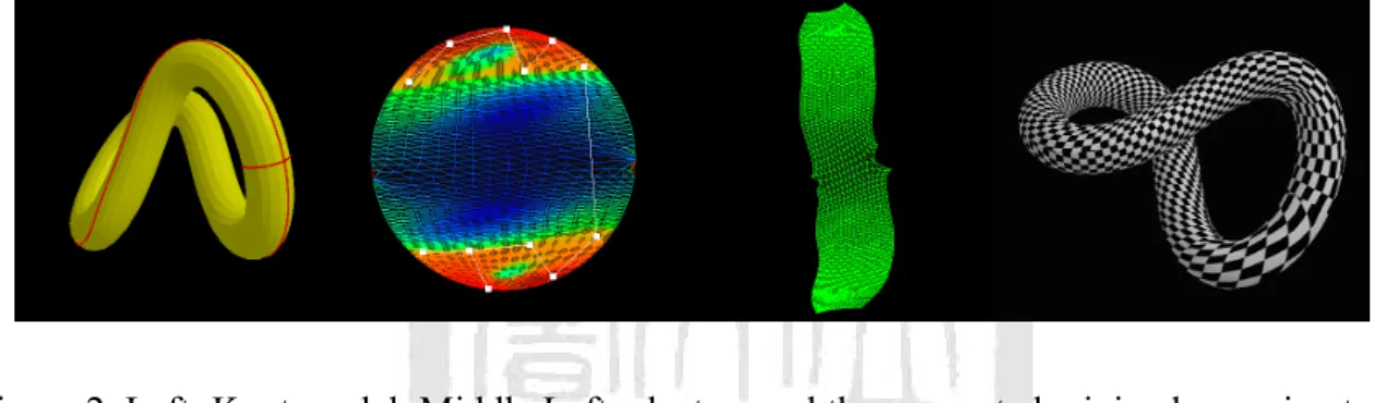
(46) Chapter 4 Constrained Texture Mapping using Partition Scheme 4.1. Overview. In computer graphics, surface parameterization is a common solution to the texture mapping problem. Parameterization commonly maps 3D meshes to a 2D domain that defines the (u, v) texture coordinates in parameterization domain. There is no isometric parameterization to map a general surface patch to a plane [1], and consequently many previous methods [7], [13], [14], [26], [29], [38], and [49] have been proposed to minimize various kind of distortion for achieving an acceptable visual effect. Most of them do not take feature matching into account. They only provide general solutions to texture mapping without constraints. However, without the correspondence of features, a 3D model with texture coordinates would look strange as shown in Figure 27. For example, the eyes on both texture and model do not match. Therefore, we need to find a method to deal with this constraint issue.. Figure 27. Texture mapping using a naïve non-constrained surface parameterization. 4.2. Parameterization with feature points. In this chapter, we develop a novel approach to texture mapping with constraints. Initially, a 28.

(47) user only needs to specify several feature correspondences between the model and the texture and then the algorithm would automatically do anything without user-interaction.. 4.2.1. Initial parameterization. We concentrate the feature-correspondence problem in this chapter. The topology of the input 3D mesh is homeomorphic to a disk. If objects are not belonging to this type, it is easy to use extra cutting to form an open disk-like surface, i.e., surface with a boundary [13]. Then, we can use any parameterization method mentioned in the related work. At the current implementation, we adopt the mean value coordinates [8] with a convex boundary in uv domain (see Figure 28 and Figure 29(c)). Figure 28 shows the weights of the mean value coordinates for each vertex of the model. If the feature points are specified on the border of models, a virtual boundary (Figure 29 (d)) can be added to the outside of the parameterized surface boundary to keep all features in the interior of the uv map. This arrangement can facilitate our method described in next section.. Figure 28. vj is the one-ring neighbor of vi for triangulation mesh. (a). (b). (c). (d). Figure 29. (a) and (b): feature correspondence between a 3D model and a texture image; (c). 29.

(48) and (d): the uv map of the mean value coordinates with and without virtual boundary start. Lt G1. G2. end. Texture. (a). P. P SP2. SP2. SP1. SP1. uv map (b). uv map (c). Figure 30. Each partitioning step determines two separate groups of features in texture and uv domains. 4.2.2. Feature matching using a partitioning approach. This section is the core of the algorithm in this chapter. The matching idea is mainly based on the procedure of the recursive partitioning in uv domain. In our setup, all computation of the matching stage is performed between the uv map and the texture. After initial parameterization, each vertex of the 3D model has an initial (u, v) coordinate. But the feature vertices don’t be matched with corresponding positions on the texture. We wrap the feature vertices to their desired positions by the partitioning approach.. Partitioning For each partitioning step, we can group the feature vertices into two disjoint sets as follows. First, feature vertices are sorted by the u (or v) coordinate on the texture domain and then the median um (or vm) is computed. Let the line segment Lt: x=um (or y=vm) be the partitioning line on the texture domain to separate the feature vertices into two groups G1 and G2 (see Figure 30(a)). Then we perform the path finding algorithm to find a path P to isolate the counterparts of G1 and G2 in the uv domain (Figure 30(b)). A path P has the same starting 30.

(49) and ending positions as those of the line Lt. Then, after partitioning by a path P, we can have two disjoint sub-patches SP1 and SP2 in the uv domain. In the next step, we align the path P with the line Lt, i.e., straightening the path P, and then re-parameterize the sub-patches SP1 and SP2 (see Figure 30(c)). A partitioning step ends. We will iteratively above partitioning tasks on the uv map until each patch contains only one feature point, say f. Finally, we will align each feature f in uv domain with its counterpart f ′ in the texture domain by a quad-partitioning of each patch as shown in Figure 31. For this purpose, we move a vertex f to a new position f ′ , i.e., correct corresponding position in texture domain. Then, we straighten all paths connecting f and four corners and re-parameterize these four sub-patches.. QP1. QP1 QP4. f QP2. f. QP4. QP2. f'. f'. QP3 QP3 (a). (b). Figure 31. The alignment of single feature f. Finding a partitioning path in uv domain First, we apply a constrained Delaunay triangulation to the uv map considering the feature vertices, S, and E (Figure 32(b)). Both S and E are the starting and ending points for a partitioning path. Second, we compute the minimal spanning trees (MST) for the group G1 and G2 (Figure 32(c)), respectively. If a MST does not exist, we will apply 1-to-4 subdivision on this triangulation map to have additional paths for finding MSTs. After finding MSTs, we find all edges, i.e., marked by X, in which one of the end points belongs to G1 and the other belongs to G2. When connecting the middle points of these edges, we can form a connected path P like Figure 32(d). Finally, the starting and ending points of P 31.

(50) connect to S and E by the shortest paths L1 and L2 to determine the final partitioning path. This partitioning path divides features into two disjoint groups in uv domain. S. S. S. 1. 3. 1. G1. 2. 2. G2. G1. 4. L1. MST 2. MST 1. 3. S. x x x. G2. G1. 4. E. E. (a) texture. (b) uv map. x xP G2 x L2. E. E. (c). (d). Figure 32. Finding a partitioning path in u,v domain. 4.2.3. UV optimization. After matching features, the uv map is distorted to some extent. The uv optimization is a process to improve the uv map as the smoothing stage in [18]. It is an iterative version of parameterization. It moves each vertex except for features within the range of one ring at each iteration to gradually minimize the distortion of uv map. We use the L2 stretch metric [32] instead of the harmonic map in [18]. In our experiment, the L2 stretch metric generally produces better results than the harmonic map (Figure 33).. 4.3. Results. We demonstrate some texture mapping results using the proposed method. Figure 33 gives the comparison between harmonic map and L2 stretch metric for the smoothing the uv map. In Figure 33, (c) yields better visual effect than (b). In Figure 34, the positions of corresponding features for an old man and a bear image are very different. The proposed method produces a not bad result. Note that in this example, we specify the features on the. 32.

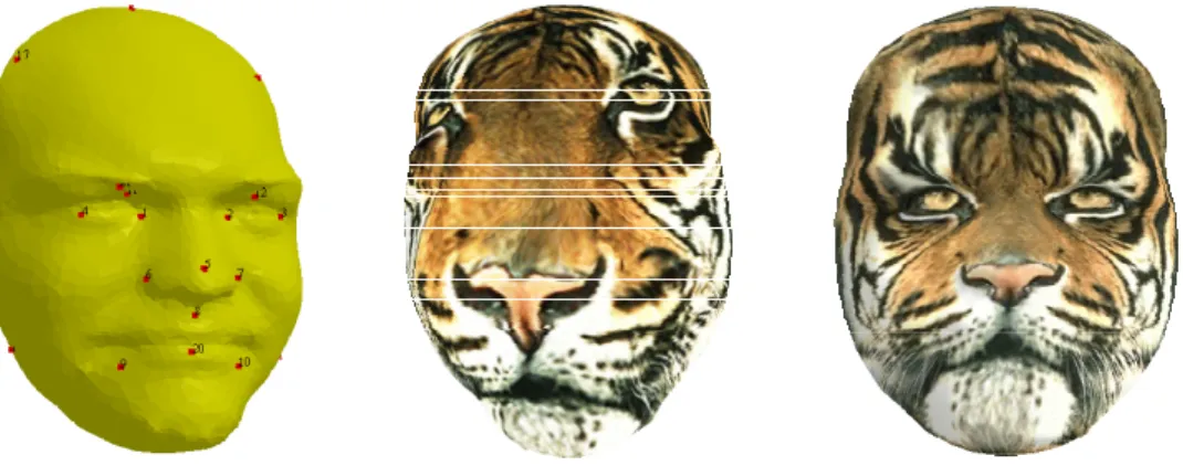
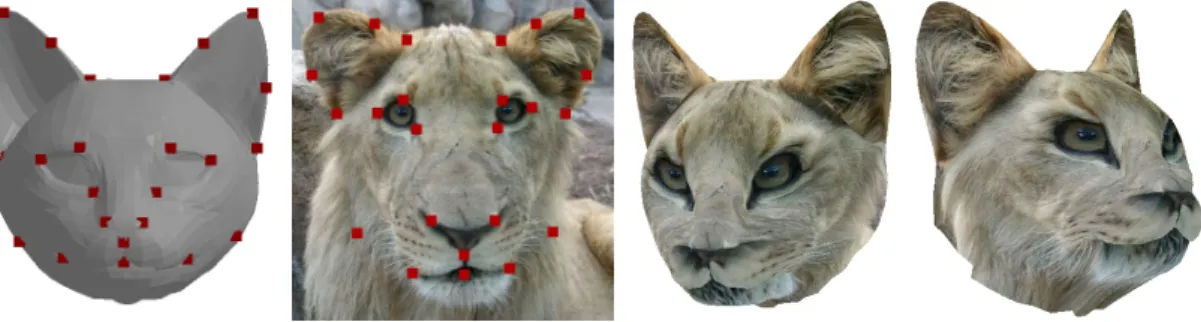
(51) border of texture image, therefore we need to add virtual boundary for the uv map. Finally, we show another interesting example in Figure 35. In this case, we do not require virtual boundary. We perform the experiments on a PC with Pentium IV 2.4 GHz and 512 MB RAM. On the average, it takes a minute to finish a texture mapping for these examples.. (a). (b). (c). Figure 33. The smoothing of uv map. (a) original texture (b) smoothed with a harmonic map (c) smoothed with L2 stretch metric. Figure 34. Texuring a man head with a bear image. Figure 35. Texturing a monkey face with a lion image. 33.

(52) Chapter 5 Constrained Texture Mapping using Warping Scheme 5.1. Overview. Texture mapping technique usually assigns (u, v) texture image coordinates to 3D mesh vertices. This assignment can be computed using mesh planar parameterization. Many other methods [3], [5], [6], [7], [14], [18], [22], [23], [26], [32], [38], and [48] have also been proposed. A more challenging problem is to compute this assignment with a special correspondence between the mesh geometry and the texture. This problem is called constrained texture mapping [3], [6], [18], [22], and [48]. The hard constraint states that the feature vertices on the parametric domain are exactly aligned to the user-specified positions. The rest of the chapter is organized as follows. We first present a foldover-free 2D mesh warping algorithm in Section 5.2, and then introduce our application to the constrained texture mapping in Section 5.3. Section 5.4 demonstrates the experimental results and gives discussion.. 5.2. Foldover-free 2D Triangle Mesh Warping. In this section, we will present a foldover-free 2D mesh warping method to satisfy positional constraints. This method uses edge swap operations to prevent triangles from folding over. The basic idea behind the proposed method is simple and well-known. However, we will show that the edge swaps must be properly arranged, otherwise, they cannot solve foldovers. To the best of our knowledge, this is the first theoretically robust algorithm for solving. 34.

(53) foldovers which uses edge swaps only. Our approach, meanwhile, can detect foldovers in advance and determine where the edge swaps should be executed to resolve potential triangle foldovers.. 5.2.1. Definitions. We consider a topologically disk-like 2D triangular mesh T with a convex boundary. The following notations are used to describe our warping algorithm. v : an interior vertex of T.. t e : an edge of T, and let e denote a line containing e. P(v ) : the union of triangles adjacent to v (see Figure 36). ∂P(v ) : the boundary (edges) of P(v ) . Q (e) : the quadrilateral formed by the two adjacent triangles sharing an edge e . Q (e) is convex if none of its internal angles is greater than π . An edge e can be swapped if Q (e) is convex. v~ : a positional constraint for v to align, and v~ is inside triangular mesh T. vm : a moving direction defined as a ray starting from v and passing through v~ , i.e., v m = vv~ . vα :. the invalid point defined as following equation. vα = arg min vp p∈K. t where K = {x | x is the intersection of vm and e , ∀e ∈ ∂P(v ) }.. 35. (1).

(54) t Eα (v ) : an edge set defined as Eα (v ) = {e | e ∈ ∂P(v ) , and e contains vα }. Our foldover-free warping algorithm gradually moves v along vm to align v~ . If vv~ ≥ vvα , we need to move v to vα first by appropriate edge-swaps and then continue. moving it to v~ gradually. The mesh therefore becomes warped. Figure 37 shows three different possibilities of vα : (a) vα is on Eα (v ) , except the vertices of Eα (v ) , (b) vα is not on Eα (v ) and (c) vα is on any vertex of Eα (v ) . We will show that v can move to vα without creating foldovers under the conditions of (a) and (b). If vα is on any vertex of Eα (v ) , we will also show that this special case can be resolved such that v can continue moving to vα along vm .. v. e. ∂P (v ). P (v ). Q (e). Figure 36. P(v ) : the union of triangles adjacent to v , ∂P(v ) : the boundary of P(v ) , and. Q (e) : the enclosing quadrilateral of e .. v. e. vα. e vm. v. v. vα e2 vm. (a) E α (v ) = {e}. (b) E α (v ) = {e}. e1. vα v m. (c) E α (v ) = { e1 , e2 }. Figure 37. ∂P(v ) consists of red edges. When v moves to vα , each shaded triangle becomes degenerated, i.e., folded over.. 36.

(55) 5.2.2. Theoretical Analysis and Algorithm. In this section, the following theoretical analysis is given, and the results of analysis are used to derive our foldover-free warping algorithm.. Theoretical Analysis Lemma 1. If |Eα(v)| = 1 and vα is on Eα(v), v can move to vα along vm without flipping triangles after an edge swap operation. Proof. vα is not on any vertex of Eα because |Eα(v)| = 1. Let Eα(v) = {e}. Then we show that e can be swapped before v moves to vα along vm . If Q(e) is convex, then e can be swapped. If Q(e) is not convex, the following statements show that e can still be swapped. In Figure 38(a), let e = p1 p3 and vp1 p 2 p3 be the quadrilateral Q(e). Both interior angles ∠p3 vp1 and ∠p1 p 2 p3 in Q(e) are less than π since they are the internal angles of triangles in 2D. triangular mesh T. Without loss of generality, let ∠p2 p3 v in Q(e) be greater than or equal to. π. Then the vertex p2 is in the shaded blue region defined by the intersection of two half-planes. These two half-planes are formed by p1 p3 and p3 v , respectively, as shown in Figure 38(a). The intersection point pi of two lines p2 p3 and vvα is on the half-closed interval [v, vα ) . If v moves to the open interval ( pi , vα ) , ∠p 2 p3 v is less than π. Then the edge e can be swapped. Since |Eα(v)| = 1, only the triangle Δvp1 p3 containing e is degenerated when v moves to vα, as shown in Figure 38(a). After e is swapped, the possibly degenerated triangle Δvp1 p3 is removed and Δvp1 p2 , as well as Δvp 2 p3 are created. Thereafter, Δvp1 p2 and Δvp 2 p3 are not flipped as v moves to vα, as shown in Figure 38(b). Our result follows.. 37.

(56) p1. p1. p1. vα. e. vα p3. v. pi. v. p3. p2. p2. (a). v. p3 p2. (b). Figure 38. (a) Eα(v) = {e}. When v moves to the open interval ( pi , vα ) , Q (e) becomes convex and e (i.e., p1 p 3 ) can be swapped. (b) edge e is swapped and v moves to vα . Lemma 2. If |Eα(v)| = 1 and vα is not on Eα(v), v can move to vα along vm without flipping triangles after an edge swap operation. Proof. Let Eα(v) = { p1 p2 }. vα is on p1 p2 , but not on p1 p2 . Without loss of generality, we assume that p2 is farther than p1 from vα . Let p3 be a vertex adjacent to both v and p2 such that vp1 p2 p3 is Q( vp2 ) as shown in Figure 39(a) and (b). The ∠p1 p2 p3 in Q( vp2 ) is not equal to π since |Eα(v)| = 1. Let p j be the intersection of vm and p2 p3 . If ∠p1 p2 p3 in Q( vp2 ) is greater than π , vα is farther than p j from v as shown in Figure 39(a). This is a contradiction to the definition of vα . Then we know that the vertex p2 is convex for. Q( vp2 ). Next we show that the edge vp2 can be swapped before v moves to vα . If the Q( vp2 ) is not convex, we will show that vp2 can be still swapped. The ∠vp1 p 2 and ∠p2 p3v in Q( vp2 ) are less than π since they are the internal angles of triangles in 2D triangular mesh T, and ∠p1 p2 p3 in Q( vp2 ) is also less than π because p2 is convex for Q( vp2 ). Then let ∠p3vp1 ≥ π in Q( vp2 ) as shown in Figure 39(b). The intersection point pi of vm and. 38.

(57) p1 p3 is on the half-closed interval [v, vα ) since ∠p3vp1 ≥ π . If v moves to the open interval ( pi , vα ) , ∠p3 vp1 < π . Then edge vp2 can be swapped. Since |Eα(v)| = 1, only the triangle Δvp1 p2 containing p1 p2 is degenerated when v moves to vα as shown in Figure 39(b). After vp2 is swapped, the possibly degenerated triangle Δvp1 p 2 is removed and Δvp1 p3 as well as Δp1 p2 p3 are created. Thereafter, Δvp1 p3 and. Δp1 p2 p3 are not flipped as v moves to vα . Our result follows.. p3. p2. p1. vm. p2. vα. vm. p1. vm. p2. p1. vα. v. pi. pj. v. v. p3. (a). p3. (b). (c). Figure 39. (a) ∠p1 p 2 p 3 > π in Q( vp 2 ). (b) ∠p 3 vp1 ≥ π in Q( vp 2 ). (c) vp2 is swapped and v moves to vα . q6 q7. q5. v. q7. q5. v. q8. q8. q1. q6. q6. vm. vα. q2. (a). q3. q4. q1. q7. q5. v. q8. vm. vα. q2. (b). q3. q4. q1. vm. vα. q2. q3. q4. (c). Figure 40. Shaded triangles are degenerated when v moves to vα . (a) Eα(v) = { q 2 q 3 , q3 q 4 , q7 q8 }. The connected components of Eα(v) are C1 = { q 2 q 3 , q3 q 4 } and C2 =. 39.

(58) { q7 q8 }. Before v moves to vα , we can swap vq4 to remove Δvq 3 q 4 as shown in (b) and then swap vq3 to remove Δvq 2 q 3 as shown in (c). Lemma 3. If |Eα(v)| ≥ 1 and vα is not on Eα(v), v can move to vα along vm without flipping. triangles after a set of edge swap operations. Proof. There are one or more connected components in Eα(v) as shown in Figure 40. For each connected component C of Eα(v), we will show that the adjacent triangle of each edge in C can be removed before v moves to vα , and then no triangles are flipped when v moves to. vα . We prove this by induction on |C| in the following. Basis Step: |C| = 1, let C = { qa qb } and follow the similar procedure of Lemma 2, i.e., let qa qb be p1 p2 as shown in Figure 39. We can find that the triangle Δvqa qb containing qa qb can be removed, and that triangles created by the swap of vqb are not degenerated when v moves to vα .. Inductive Step: We assume the statement is true while |C| = k. Now consider |C| = k + 1 . First, all edges of C are collinear since C ⊆ Eα and C is connected. Let qs qt ∈ C. Without loss of generality, qs qt is the farthest element of C from vα , and qt is farther than qs from vα . If we follow the similar procedure as that used in Lemma 2, i.e., let qs qt be p1 p2 as shown in Figure 39. The triangle Δvq s qt containing qs qt can be removed, and the new triangles created by edge swap of vqt are not degenerated when v moves to vα , and then |C| = k. Using the induction hypothesis, the adjacent triangle of each edge in C can be removed as shown in Figure 40. Our result follows.. 40.

(59) u′m. vm v. u(vα ). u′m. u′α. vm u(vα ). v. u′α. vm. u v. Figure 41. (a) vα is on a vertex u of Eα(v). u can find a direction um′ in (b). Then u can move to the interval (u, uα′ ) and v can move to vα in (c). Lemma 4. If |Eα(v)| ≥ 1 and vα is on Eα(v), but not on the vertices of Eα(v), v can move to vα along vm without flipping triangles after a set of edge swap operations. Proof. We will show that the adjacent triangle of each edge in Eα(v) can be removed before v moves to vα , and that no triangles are flipped when v moves to vα . We classify the edges of. Eα(v) into two sets B1, and B2 . (a) B1 = { qi q j | qi q j ∈ Eα(v) and vα is on qi q j }. Then |B1| = 1 because vα can be on one edge of Eα(v) at most. Let B1 = { qm qn }, we can follow the similar procedure as that used in Lemma 1, i.e., let qm qn be the edge e as shown in Figure 38. Then we can find that qm qn can be swapped to remove the triangle Δvqm qn , and that the new triangles created by the edge swap of qm qn are not degenerated when v moves to vα . (b) B2 = { qi q j | qi q j ∈ Eα(v) and vα is not on qi q j }. By following the similar procedure of Lemma 3, the adjacent triangle of each edge in B2 can be removed and the new triangles are not degenerated when v moves to vα . Our result follows. Lemma 5. If vα is on a vertex u of Eα(v), v can move to vα along vm without flipping. 41.

(60) triangles. Proof. We first show that u can be temporarily moved, such that u is not on the direction of. vm . We create a moving direction um′ for u by randomly picking a direction that is not the same as vm and − vm as shown in Figure 41(a). Then u can find a temporary invalid point. uα′ by um′ . If u moves to the open interval (u, uα′ ) , u is not on the direction of vm and no triangles are flipped. Then by Lemma 3 or Lemma 4, v can continue moving to vα as shown in Figure 41(c). Our result follows. In addition, Figure 41(c) shows that u can also move back to vα along − um′ to restore its original position by Lemma 3 or Lemma 4 after v leaves vα along vm . We can state the following theorem from Lemma 3, Lemma 4, and Lemma 5. Theorem 1. v can move to the invalid point vα along vm without flipping triangles.. Foldover-free Warping Algorithm Now, we will describe a foldover-free 2D mesh warping algorithm in MeshWarp() based on the above analysis. Iteratively, this algorithm moves each vertex v along vm to v~ . If v is required to move to vα , the algorithm executes edge swaps to remove possibly degenerated triangles. Then v moves to vα using MoveToInvalidPoint(v). The procedure. MoveToInvalidPoint() is derived from Lemma 3, Lemma 4, and Lemma 5. Note that the StepSpeed in MeshWarp() is a user-defined constant to control the warping speed and MinimalStep(T) returns the minimal distance between each vv~ for all un-aligned vertices. In our experiment, if the StepSpeed constant is set too large, the number of edge swaps would. 42.

(61) become bigger and the large distortion would occur in base mesh. From our experimental experience, the value 0.1 is a good constant for the StepSpeed.. 43.

(62) 44.