Elsevier Editorial System(tm) for Expert Systems With Applications
Manuscript Draft
Manuscript Number:
Title: An Improved Data Mining Approach Using Predictive Itemsets Article Type: Full Length Article
Keywords: data mining, association rule, predictive itemset, data dependency, predicting minimum support
Corresponding Author: Professor Tzung-Pei Hong, PhD
Corresponding Author's Institution: National University of Kaohsiung First Author: Tzung-Pei Hong, PhD
Order of Authors: Tzung-Pei Hong, PhD; Chyan-Yuan Horng; Chih-Hung Wu; Shyue-Liang Wang
An Improved Data Mining Approach Using Predictive Itemsets
Tzung-Pei Hong1*, Chyan-Yuan Horng2, Chih-Hung Wu3, Shyue-Liang Wang41Department of Electrical Engineering, National University of Kaohsiung Kaohsiung, 811, Taiwan, R.O.C.
2Institute of Information Engineering, I-Shou University Kaohsiung, 840, Taiwan, R.O.C.
3Department of Information Management, Shu-Te University Kaohsiung, 824, Taiwan, R.O.C.
4Department of Computer Science, New York Institute of Technology New York, USA
ABSTRACT
In this paper, we present a mining algorithm to improve the efficiency of finding large itemsets. Based on the concept of prediction proposed in the (n, p) algorithm, our method considers the data dependency in the given transactions to predict promising and non-promising candidate itemsets. Our method estimates for each level a different support threshold that is derived from a data dependency parameter and determines whether an item should be included in a promising candidate itemset directly. In this way, we maintain the efficiency of finding large itemsets by reducing the number of scanning the input dataset and the number candidate items. Experimental results show our method has a better efficiency than the apriori and the (n, p) algorithms when the minimum support value is small.
Keywords: data mining, association rule, predictive itemset, data dependency, predicting minimum support.
--- * Corresponding author Manuscript
1. Introduction
Years of effort in data mining have produced a variety of efficient techniques. Depending on the types of datasets processed, mining approaches may be classified as working on transaction datasets, temporal datasets, relational datasets, or multimedia datasets, among others. On the other hand, depending on the classes of knowledge derived, mining approaches may be classified as finding association rules, classification rules, clustering rules, or sequential patterns [2], etc. Among these techniques, finding association rules from transaction datasets is usually an essential task [1][3][5][10][12][17][19][22][23][24].
Many algorithms for mining association rules from transactions are proposed, most of which are executed in level-wise processes. That is, itemsets containing single items are processed first, then itemsets with two items are processed. The process was repeated, continuously adding one more item each time, until some criteria are met. The famous apriori mining algorithm was proposed by Agrawal et al. [4][5]. The apriori iterates two phases, the phase of candidate generation and the phase of verification. Possible large itemsets are produced in the first phase and verified in the second phase by scanning the input dataset. Since itemsets are processed level by level and datasets had to be scanned in each level, the verification phase thus dominates the performance. Han et al. then proposed the Frequent-Pattern-tree (FP-tree) structure for efficiently mining association rules without
generation of candidate itemsets [13]. The FP-tree was used to compress a database into a tree structure which stored only large items. Several other algorithms based on the FP-tree structure have also been proposed. For example, Qiu et al. proposed the QFP-growth mining approach to mine association rules [20]. Zaiane and Mohammad proposed the COFI-tree structure to replace the conditional FP-tree [25]. Ezeife constructed a generalized FP-tree, which stored all the large and non-large items, for incremental mining without rescanning databases [10]. Koh et al. adjusted FP trees also based on two support thresholds [15], but with a more complex adjusting procedure and spending more computation time than the one proposed in this paper.
In [9], Denwattana and Getta proposed an algorithm (referred to as the (n, p) algorithm) to reduce the numbers of scanning input datasets for finding large itemsets. The (n, p) algorithm also iterates two phases, the phase of prediction and the phase of verification. Unlike the apriori, the (n, p) algorithm predicts large itemsets for p levels in the first phase and verifies all these p-level itemsets in the second phase. A heuristic estimation method is presented to predict the possibly large itemsets. If the prediction was valid, then the approach is efficient in finding the actually large itemsets.
In this paper, we propose a mining algorithm to improve the efficiency of finding large itemsets. Our approach is based on the concept of prediction presented in the (n, p) algorithm and considers the data dependency among transactions. As the (n, p) algorithm does, our
method iterates the same two phases but uses a new estimation method to predict promising and non-promising candidate itemsets flexibly. The estimation mechanism computes for each level a different support threshold derived from a data dependency parameter and determines whether an item should be included in a promising candidate itemset directly by the support values of items. Since we reduce the number of candidate itemsets to be verified by the new estimation mechanism and the number of scanning of the input dataset by the concept of prediction of the (n, p) algorithm, the performance of finding large itemsets can be improved. The rest of this paper is organized as follows. Section 2 presents the related works of finding large itemsets. The apriori algorithm and the (n, p) algorithm are reviewed. In Section 3, we describe our motivation and the theoretical foundation of our method. Detailed description of our algorithm is given in Section 4 together with a simple example. Experimental results and the comparison on the performance of the apriori, the (n, p) algorithm, and our method are shown in Section 5. Conclusions are given in Section 6.
2. Related Works
One application of data mining is to induce association rules from transaction data, such that the presence of certain items in a transaction will imply the presence of certain other items. Below we briefly reviewed the apriori and the (n, p) algorithm.
2.1. The Apriori Algorithm
Agrawal et al [1][3][5] proposes a famous mining algorithm, the apriori, based on the concept of large itemsets to find association rules in transaction data. The apriori iterates two phases, the phase of candidate generation and the phase of verification, at each level. At the i-th level, i>1, itemsets consisting of i-items are processed. In candidate generation, all possible large i-itemsets are produced by combining the unrepeated elements of (i-1)-itemsets. In the verification phase, the input dataset is scanned and if the number of an i-itemset appearing in the transactions is larger than a pre-defined threshold (called the minimum support, or minsup), the itemset is considered as large. After that, these two phases iterate for (i+1)-level until all large itemsets are found.
Suppose that we have a dataset containing 6 transactions, as shown in Table 1, which has two features, transaction identification (ID) and transaction description (Items). There are eight items in the dataset. Assume that minsup=30%. The transaction dataset is first scanned to count the candidate 1-itemsets. Since the counts of the items a(4), b(5), c(6), d(3), and e(4) are larger than 6*30%=1.8, they are thus put into the set of large 1-itemsets. Candidate 2-itemsets are then formed from these large 1-itemsets by taking any two items in the large 1-itemsets and counting if their occurrences are large than or equal to 1.8. Therefore, ab, ac, ae, bc, bd, be, cd, ce, and de then form the set of large 2-itemsets. In a similar way, abc, abe, ace, bce, bcd, bde, and cde form the set of large 3-itemsets, abce and bcde form the set of
large 4-itemsets.
Table 1. A sample dataset of transactions ID Items 1 a b c 2 b c d e f 3 a b c e g 4 a c d 5 b c d e 6 a b c e
2.2. Denwattana and Getta’s Approach
In [9], the (n, p) algorithm tries to reduce the number of scanning datasets and improves the efficiency of finding large itemsets by “guessing” what items should be considered. The approach partitions candidate itemsets into two parts: positive candidate itemsets and negative candidate itemsets, where the former contains itemsets guessed to be large and the later contains itemsets guessed to be small. Initially, the (n, p) algorithm scans the dataset to find large itemsets of 1-items. Two parameters, called n-element transaction threshold tt and
frequency threshold tf, are used to judge whether an item could compose a positive candidate
itemset. According to the n-element transaction threshold tt, only the transactions with item
numbers (lengths) less than or equal to tt are considered. The frequency of each item
appearing in transactions with j items, j ≤ tt,, is computed. If the appearing frequency of an
item is larger than or equal to tf, the item could be used to compose a positive candidate
In the prediction process, positive candidate 2-itemsets C , each of which has its two items 2+ satisfying the above criteria, is formed. The remaining candidate 2-itemsets not in C form 2+
−
2 C . +
3
C and C3− are then formed from only C2+ in a similar way. The positive candidate 2-itemsets which are subsets of the itemsets in +
3
C are then removed from C . The same 2+ process was repeated until p levels of positive and negative candidate itemsets are formed. After that, the verification process check whether the itemsets in the positive candidate itemsets are actually large and the itemsets in the negative candidate itemsets are actually small by scanning the dataset once. The itemsets incorrectly guessed are then expanded and processed by scanning the dataset again.
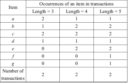
Consider the dataset shown in Table 1 again. Suppose that minsup=30% and the n-element transaction threshold tt=5 and (n, p)=(5, 3). The numbers of occurrences of each
Table 2. The number of occurrences of each item in transactions of different lengths
Assume the frequency threshold tf =80%. The occurrence number of each item in
transactions with 3 items must be larger than or equal to 1.6 (2*80%) for this item to be considered as positive. Thus, items a and c are positive. Similarly, b, c, and e are positive for transactions with 4 items, and b, c, and e are positive for transactions with 5 items. The items which can be used to compose positive candidate itemsets are thus the union {a, b, c, e} of the above three sets . We obtain C ={bc, be, ab, ce, ac, ae}, and 2+ C ={bd ,bf, bg, cd, cf, cg, 2− de, ef, eg, ad, af, ag, df, dg, fg}. Then, +
3
C and −
3
C are formed from +
2 C as +
3
C ={bce, abc, abe, ace}, and −
3
C =φ. C4+ and C are formed from 4− C3+ as C4+={abce}, and C4−=φ. The elements in +
2
C which are subsets of those in +
3
C are removed. Thus, we obtain +
2
C =φ. Similarly, the itemsets in +
3
C which are subsets of those in C4+ are removed. Therefore,
+
3
C =φ.
Occurrences of an item in transactions Item
Length = 3 Length = 4 Length = 5
a 2 1 1 b 1 2 2 c 2 2 2 d 1 1 1 e 0 2 2 f 0 0 1 g 0 0 1 Number of transactions 2 2 2
In the verification process, the dataset is scanned to check all the itemsets in +
j
C and
−
j
C , j=2,3,4. After the scan, the set of large itemsets in positive candidate sets is {abce}. The
set of small itemsets in negative candidate sets is {bf, bg, cf, cg, ef, eg, ad, af, ag, df, dg, fg}. The itemsets de, cd, and bd in −
2
C are incorrectly predicted. The incorrectly predicted
itemsets are further processed. The subsets of incorrectly predicted itemsets in positive candidate sets are first generated. These subsets are then pruned using the large itemsets already known. Since +
4
C is correctly predicted, the result is φ. The supersets of incorrectly
predicted itemsets in negative candidate sets are also generated as {bde, cd, cde, bcde}. The dataset is then scanned again to check these itemsets. Therefore, the itemset {bcd, bde, cde, bcde} is large in the second scan. All the large itemsets are then collected as:
L2={bd, cd, de, ae, ac, ce, ab, be, bc}
L3={cde, bde, bcd, ace, abe, abc, bce}
L4={bcde, abce}
The same process goes on for finding L5 to L7. C5 is first generated from L4 as {abcde}
and checked to be large in the same manner. After all the large itemsets are found, the association rules can then be derived from them.
3. Motivation
3.1. Observation
The apriori algorithm is straightforward and simple but needs to repeatedly scan the dataset while finding the large itemsets. There have been many approaches proposed to reduce the number of scanning datasets. The (n, p) algorithm is one of such approaches. It scans the input dataset once in the beginning and twice in each verification process. Since p levels of transactions are processed in an iteration, the number of scanning datasets is less than that in the apriori. In the above example, the apriori scans the dataset 10 times; while the (n, p) algorithm scans 5 times. In [9], it is claimed that the number of scanning the dataset can be reduced with proper parameters n and p.
Unfortunately, in some cases, the overall performance of the (n, p) algorithm is defected because of the verification process. In +
i
C and Ci−, i ≥2, all itemsets with lower supports are rejected by +
i
C and are collected into Ci−. When generating Ci++1 and Ci−+1, all elements in
+
i
C and Ci− are taken into account, respectively. If there are a large number of itemsets with supports lower than the pre-defined minsup and are included in −
i
C , the (n, p) algorithm also
has to compute all combinations of such itemsets and deletes them all in the verification process. This affects the overall performance of the (n, p) algorithm. On the other hand, in using the apriori, only the itemsets with supports higher than minsup are considered. For example, the (n, p) algorithm guesses that 200 out of 1000 2-itemsets are large and included in +
2
C and 800 items are in C2−; 70% elements in C2+ and 99% elements in C2− are not large enough. It takes about (800×99%)2(k -1) computations in generating −
k
and removes most elements in −
k
C in the verification phase. In the apriori, if 200×120%
2-itemsets are actually large (the (n, p) algorithm may make a wrong guess), only (200×120%)2 computations are needed in generating +
3
C and much less than (200×120%)2
are left after verifying their supports by scanning the dataset. Though the number of scanning the dataset in the (n, p) algorithm is less than that in the apriori, the overall performance of the (n, p) algorithm may be not good enough. Experimental results are available in Section 5. Therefore, the performance of the (n, p) algorithm can be further improved. One direction of improvement is to employ better data structures, so that the generation of +
+1 i
C and Ci−+1 can be done in a more efficient manner, such as [6][7][15][18][26]. The other direction is filtering out the itemsets with lower supports and reduce the number of elements to be included in +
i
C
and −
i
C . This paper adopts the later approach from a point of view of probability.
3.2. Theoretical Foundation
Usually, items must have greater support values for being covered in large itemsets with more items from a probabilistic viewpoint. For example, if minsup is 30%, then an item with its support just greater than 30% is a large 1-itemset. Both items in a 2-itemset must, however, have their supports a little larger than 0.3 for this 2-itemset to be large with a high probability. At one extreme, if total dependency relations exist in the transactions, an appearance of one item will certainly imply the appearance of another. In this case, the support thresholds for an
item to appear in large itemsets with different items are the same. At the other extreme, if the items are totally independent, then the support thresholds for an item to appear in large itemsets with different items should be set at different values. In this case, the support threshold for an item to appear in a large itemset with r items can be easily derived below.
Since all the r items in a large r-itemset must be 1-large itemsets, all the supports of the r items must be larger than or equal to the predefined minsup α. Since the items are assumed totally independent, the support of the r-itemset is s1× s2× …× sr, where si is the actual
support of the i-th item in the itemset. If this r-itemset is large, its support must be larger than or equal to α. Thus:
s1× s2× …× sr ≥α.
If the predictive support threshold for an item to appear in a large r-itemset is αr, then:
s1× s2× …× sr ≥αr×αr× …×αr ≥α.
Thus:
α
α
r ≥r and αr≥α1/r.
Therefore, if the items are totally independent, the support threshold of an item should be expected to be α1/r for being included in a large r-itemset. Since the transactions are seldom totally dependent or totally independent, a data dependency parameter w, ranging between 0 and 1, is then used to calculate the predictive support threshold of an item for appearing in a large r-itemset as wα+(1-w)α1/r. A larger w value represents a stronger item relationship
existing in transactions. w=1 means total dependency for transaction items and w=0 means total independency. The proposed approach thus uses different predictive support thresholds for each item to be included in promising itemsets with different numbers of items.
4. Our Method
4.1. Our Algorithm
The proposed mining algorithm aims at efficiently finding any p levels of large itemsets by scanning a dataset twice except for the first level. The support of each item from the first dataset scan is directly judged to predict whether an item will appear in an itemset. The proposed method uses a higher predicting minsup for each item to be included in a promising itemset of more items. Itemsets with different numbers of items then have different predicting minsups for an item. A predicting minsupt is calculated as a weighted average of the possible minsups for totally dependent data and for totally independent data. A data dependency parameter, ranging between 0 and 1, is used as the weight.
A mining process similar to that proposed in [9] can then be adopted to find the p levels of large itemsets. A dataset is first scanned to get the support of each item. If the support of an item is larger than or equal to the predefined minsup value, it is put in large 1-itemsets L1.
After large 1-itemsets have been found, any more p levels of large itemsets can be obtained by scanning a dataset twice. Candidate 2-itemsets (C2) are formed by combination of the
items in large 1-itemsets. In the meantime, the predicting minsup for an item to be included in large 2-itemsets is estimated according to the given data dependency parameter. If the support of an item in L1 is smaller than the predicting minsup, any candidate 2-itemset including this
item will not be large with a high possibility. On the contrary, any candidate 2-itemset with supports of all items larger than or equal to the predicting minsup will have a high possibility of being large. The candidate 2-itemset can then be partitioned into two parts: +
2
C and C2−, according to whether the supports of all the items in an itemset are larger than or equal to the predicting minsup.
After promising candidate 2-itemsets ( +
2
C ) are generated, candidate 3-itemsets (C3) are
formed by the combining them. Similar to the process for finding candidate 2-itemsets, a new predicting minsup for each item to be included in promising 3-itemsets is calculated. Candidate 3-itemsets can then be partitioned into two parts: +
3
C and C3− by comparing the supports of the items included in C3 with the predicting minsup. The same procedure is
repeated until the p levels of itemsets are processed. Therefore, no dataset scan except for the first level has been done until now. A dataset is then scanned to get the actually large itemsets in the promising candidate itemsets and in the non-promising candidate itemsets. The itemsets incorrectly predicted in the p levels are further processed by scanning the dataset once more. Therefore, a total of two dataset scans are needed in getting the p level large itemsets. After that, another processing phase of p levels is done. This processing is repeated
until no large itemsets are found in a phase. Let ci be the number of occurrence of each item
ai appearing in the input dataset of transactions and the support (αi) of each item ai be ci /n.
INPUT: A set of n transactions with m items, the minsup α, a dependency parameter w, and a level number p.
OUTPUT: Large itmesets.
STEP 1: Check whether the support αi of each item ai is larger than or equal to α. If αi≥α, put ai in
the set of large 1-itemsets L1.
STEP 2: Set r=1, where r is the number of items in itemsets currently being processed. STEP 3: Set r’=1, where r’ is the number of items at an end of the last iteration. STEP 4: Set Pr = Lr, where Pr is the items predicted to be included in r-itemsets. STEP 5: Generate the candidate set Cr+1 from Lr in a way similar to that in the apriori. STEP 6: Set r=r+1.
STEP 7: Check whether the support αi of each item ai in Pr-1 is larger than or equal to the predicting
minsup α’=wα+(1-w)α1/r to be included in Pr. If αi≥α’, put ai in Pr.
STEP 8: Form the promising candidate itemsets C by choosing from Cr+ r the itemsets with each
item existing in Pr.
STEP 9: Set the non-promising candidate itemsets Cr− =Cr−Cr+.
STEP 10: Set r=r+1.
STEP 11: Generate the candidate set Cr from Cr+−1 in the way as the apriori does.
STEP 12: Check whether the support αi of each item ai in Pr-1 is larger than or equal to the predicting
minsup α’=wα+(1-w)α1/r. If α
i≥α’, put ai in Pr.
STEP 13: Set the non-promising candidate itemsets Cr−=Cr−Cr+.
STEP 14: Remove the itemsets in Cr+−1, which are subsets of any itemset in C . r+
STEP 15: Repeat STEP 10 to STEP 14 until r = r’ + p.
STEP 16: Scan the dataset to check whether the promising candidate itemsets, Cr+'+1 to Cr+ are actually large and whether the non-promising candidate itemsets, Cr−'+1 to Cr− are actually small. Put the actually large itemsets in the corresponding sets Lr’+1 to Lr.
STEP 17: Find all the proper subsets with r’+1 to i items for each itemset which is not large in C , r’ i+ +1 ≤i ≤r; keep the proper subsets which are not among existing large itemsets; donate them
as NC+.
STEP 18: Find all the proper supersets with i to r items for each itemset which is large in C , r’ +1 i− ≤
i ≤ r; the supersets must also have all their sub-itemsets of r’ items existing in Lr’ and cannot
include any sub-itemset in the non-large itemsets in C and i+ C checked in STEP 16; i−
donate them as NC-.
STEP 19: Scan the dataset to check whether the itemsets in NC+ and NC- are large; add the large
itemsets to the corresponding sets Lr’+1 to Lr.
STEP 20: If Lr is not null, r’= r’ + p and go to STEP 4 for another iteration; otherwise do STEP 21. STEP 21: Add the non-redundant subsets of large itemsets to the corresponding sets L2 to Lr.
4.2. An Example
In this section, the dataset in Table 1 is used to describe our method. Assume that minsup α= 30% and w=0.5 in this example. The following processes are performed.
STEP 1: The support of each item is compared with the minsup α. Since the supports of {a}, {b}, {c}, {d}, and {e} are larger than or equal to 0.30, they are put in L1.
STEP 2: r=1. STEP 3: r’= 1.
STEP 4: P1is the same as L1, which is {a, b, c, d, e}.
STEP 5: The candidate set C2 is formed from L1 as C2 = {ae, be, ce, de, ad, bd, cd, ac, bc,
ab}.
STEP 6: r = r + 1 = 2.
STEP 7: The predicting minsup value for each item α’=0.5×0.30+(1-0.5)×0.301/2=0.424. The support of each item in P1 is then compared with 0.424. Since the supports
of {a}, {b}, {c}, {d}, and {e} are larger than 0.424, P2is {a, b, c, d, e}.
STEP 8: The itemsets in C2 with each item existing in P2 are chosen to form promising
candidate itemsets +
2
STEP 9: The non-promising candidate itemsets −
2
C is found as C = 2− C -2 C = 2+ φ.
STEP 10: r = r + 1 = 3.
STEP 11: The candidate set C3 is formed from C as C2+ 3 = {abe, ace, ade, bce, bde, cde, abd, acd, bcd, abc}.
STEP 12: The predicting minsup α’=0.5×0.30+(1-0.5)×0.301/3=0.485. The support of each item in P2 is then compared with 0.485. Since the supports of {a}, {b}, {c}, {d}
and {e} are larger than 0.485, P3 is {a, b, c, d, e }. Thus, we have C3+= C3.
STEP 13: The non-promising candidate itemsets C3− is found as C3− = C3-C3+ = φ.
STEP 14: Since all itemsets in +
2
C are subsets of itemsets in +
3
C , they are removed from
+
2 C =φ.
STEP 15: Since r (=3) < r’ + p (=4), STEP 10 to STEP 14 are repeated. r = 3+1 = 4. The candidate set C4 is then formed from C3+ as C4 = {abce, abde, acde, bcde, abcd}. The predicting minsup value α’=0.5×0.30+(1-0.5)×0.301/4=0.520. The support of each item in P3 is then compared with 0.520. Since the supports of
{a}, {b}, {c}, and {e} are larger than 0.520, P4 is {a, b, c, e}. C4+ is thus formed as C4+ = {abce}. The non-promising candidate itemsets C4− is found as
−
4
C = C4- +
4
C = {abde, acde, bcde, abcd}. The itemsets in +
3
C which are subsets of itemsets in +
4
C are removed from +
3
C . Thus, we obtain +
3
C ={ade, bde, cde, abd, acd, bcd}.
STEP 16: The dataset is scanned to check whether the promising candidate itemsets of C2+ to C4+ are actually large and whether the non-promising candidate itemsets of
−
2
C to −
4
C are actually small. The itemsets ad in +
2
C , ade, abd, acd in +
3 C , and bcde in −
4
C are incorrectly predicted. By deleting ad, ade, abd, and acd from
+
2
C and C3+, the rest of elements in C2+, C3+, and C4+ are put into L2, L3, and L4, respectively. Also, bcde is put into L4.
STEP 17: The proper subsets of the itemsets incorrectly predicted in Ci+ are generated. Since {ad, ade, abd, acd} is incorrectly predicted in this example, its proper subsets not in existing large itemsets is {ad}. Thus NC+ = {ad}.
STEP 18: The proper supersets of the itemsets incorrectly predicted in −
i
C are generated. Since only {bcde} is incorrectly predicted in this example, its proper supersets with 3 items and not in existing large itemsets is φ. Thus NC-=φ.
STEP 19: The dataset is scanned to find the large itemsets from NC+ and NC-. Since {ad}
is not large by verifying the dataset, the large itemsets L2 to L4 are then found as
L2={ab, bc, ac, cd, bd, de, ce, be, ae}, L3={abc, bcd, cde, bde, bce, ace, abe},
and L4={bcde, abce}.
STEP 20: Since L4 is not null, the next iteration is executed. STEP 4 to STEP 19 are then
repeated for L5 to L7. Then, we have C5 = {abcde} and L5 = L6=L7 = φ.
corresponding sets L2 to L4. The final large itemsets L2 to L4 are then found as
follows:
L2={ab, bc, ac, cd, bd, de, ce, be, ae},
L3={abc, bcd, cde, bde, bce, ace, abe}
L4={bcde, abce}
5. Experiments and Results
In order to demonstrate the performance of our method, several experiments are performed. All the three methods, the apriori, the (n, p) algorithm, and our method, are implemented in Java using the same data structure and representation. The experiments are performed on a personal computer with a Pentium-IV 2.0 GHz CPU and Windows™. We collect different types of datasets using the data generator provided by [14]. The following parameters indicate the contents of the dataset.
z nt: the number of transactions in dataset
z lt: average transaction length in the dataset
z ni: the number of items in the dataset
z np: the number of patterns found in the dataset
z lp: average length of pattern
z cp: correlation between consecutive patterns
z f: average confidence in a rule z vc: variation in the confidence
used in generating a dataset D.
5.1. Experiment I
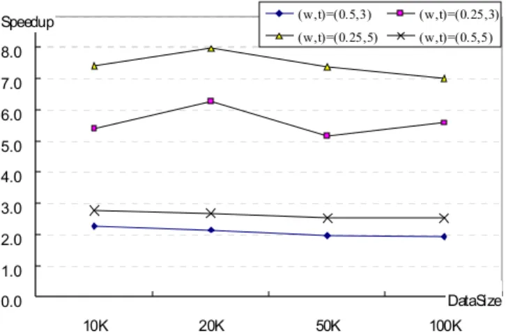
First of all, we test if our algorithm performs better than the apriori does. The dataset D1
is generated with the parameters (D1, nt, 10, 25, 1000, 4, 0.15, 0.25, 0.1). We perform the two
programs with different sizes, nt=10K, 20K, 50K, 100K, of datasets and compare the
performance by speedup which is computed as (tp-to/to), where tp is the running time of the
apriori and to is the running time of ours. In this experiment, the minsup is set at 15% and
different combinations of the data dependency parameter w and transaction threshold t are tested. The experimental result is shown in Figure 2. It seems that our method is scalable and provides a better computational performance than the apriori with a lower w.
0.0 1.0 2.0 3.0 4.0 5.0 6.0 7.0 8.0 9.0 10K 20K 50K 100K DataSize Speedup (w,t)=(0.5,3) (w,t)=(0.25,3) (w,t)=(0.25,5) (w,t)=(0.5,5)
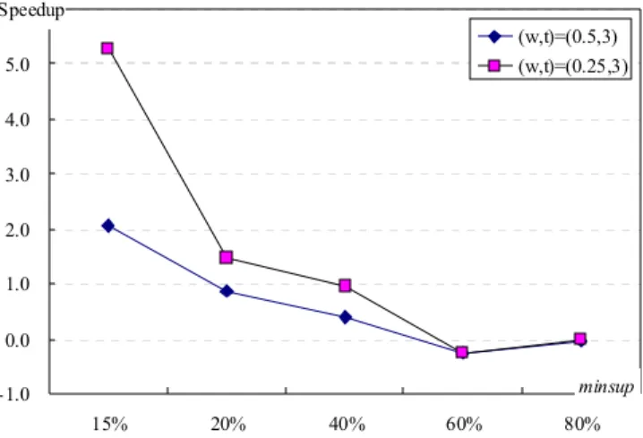
5.2. Experiment II
Next, the dataset D1 is used to test the performance of our method with different values
of minsup. We set nt=10000. The speedup is illustrated in Figure 3. Like the (n, p) algorithm,
our algorithm has a better performance when minsup is low. This is because that the apriori exactly filters out itemsets with supports lower than minsup in each stage and reduces the number of elements to be considered in generating candidate itemsets. In the (n, p) algorithm and ours, we have to guess what itemsets should be considered in the prediction phase and then to verify the predicted ones. The generation of proper subsets and supersets after the verification phase takes a considerable time.
-1.0 0.0 1.0 2.0 3.0 4.0 5.0 6.0 15% 20% 40% 60% 80% minsup Speedup (w,t)=(0.5,3) (w,t)=(0.25,3)
Figure 3. Speedup in experimental result II with different minsup
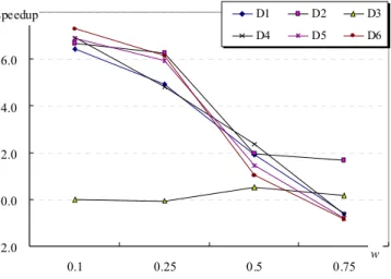
5.3. Experiment III
According to experiments I and II, we find that the performance of our method is sensitive with respect to the contents of the datasets, i.e, the relationships among data in the
datasets. We generated 5 different datasets, D2, D3, D4, D5, D6 by the changing cp and f and
remaining the rest parameters the same as that in D1. The parameters (cp, f) in D2, D3, D4, D5,
and D6 are given as (0.05, 0.75), (0.05, 0.25), (0.15, 0.75), (0.25, 0.75), and (0.25, 0.25),
respectively. Figure 4 presents the results with 10000 data in each dataset.
-2.0 0.0 2.0 4.0 6.0 8.0 0.1 0.25 0.5 0.75 w speedup D1 D2 D3 D4 D5 D6
Figure 4. Experimental result on different datasets
The data dependency parameter w seems to have an effect on the performance of the proposed algorithm, but not on the final large itemsets. A larger w value represents a stronger item relationship existing in transaction datasets. If the relationships of data items in transactions have been known to be very strong, w may be set at a value close to 1. If the relationships of data items in transactions have been known to be independent, w may be set at a value close to 0. If the relationships of data items in transactions are unknown, w may be set at 0.5.
respectively. Assume w=0 and minsup=30%, we obtain L1= {a, b, c, d, e} and +
2
C ={ae, be, ce, ac, bc, ab},
+ 3 C = + 4 C = φ, − 2 C = {cd, bd, ad, de}, − 3
C = {bce, ace, abe, abc},
−
4 C =φ.
The itemsets that are incorrectly predicted are cd, bd, de, bce, ace, abe, and abc. L3 and
L4 are generated from the supersets of NC-={cd, bd, de} and NC-={bce, ace, abe, abc},
respectively. If w = 1, we obtain L1= {a, b, c, d, e} and + 2 C = + 3 C =φ, + 4
C = {abce, abde, acde, bcde, abcd},
− 2 C = − 3 C = − 4 C =φ,
The itemsets that are incorrectly predicted are abde, acde, and abcd. L2 and L3 are
generated from the subsets of NC+={abde, acde, abcd}. In both cases, many computations are spent in combining the items from NC+(NC-). Generally, w = 0.5 has a better performance than w = 0 or w = 1.
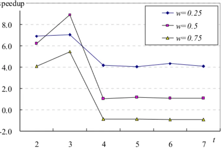
5.4. Experiment IV
performance. The dataset D2 is used to test. It seems that the best performance appear when 3
levels are considered in an iteration. Also, it is found that the data in D2 are of low
dependency (cp=0.05). This is because that the generation of Ci++1 from Ci+ is of O(m2) computational complexity, where m is the number of elements in +
i
C . The more levels of transactions are considered in an iteration the larger n may be obtained.
-2.0 0.0 2.0 4.0 6.0 8.0 10.0 2 3 4 5 6 7 t speedup w=0.25 w=0.5 w=0.75
Figure 5. Experimental result on different levels of transactions
6. Discussions and Conclusions
From the experimental results, different values of data dependency will cause the same large itemsets, but different predictive effects. When w=1, the non-promising candidate sets are predicted very well, but the promising candidate sets are predicted badly; and vice versa for w=0. By default, we set w=0.5. If the data dependency relationships in transactions can be well utilized, our method can improve the overall performance of finding large itemsets.
generating + +1 i
C from +
i
C . When there are many items in the dataset, e.g., 25 items in D1~D6, and more levels of transactions to be considered, more computation is needed in both
algorithms. However, our method provides a more accurate approach for predicting itemsets and obtains a better performance than the (n, p) algorithm, especially when p>2.
In this paper, we have presented a mining algorithm that combines the advantages of the apriori and the (n, p) algorithm in finding large itemsets. As the (n, p) algorithm does, our algorithm reduces the number of scanning datasets for finding p levels of large itemsets. A new parameter that considers data dependency is included in our method for early filtering out the itemsets that are possibly of lower supports and thus improves the computational efficiency.
We also conclude that the three algorithms can compete with each other and gain the best performance on different types of datasets. There need more studies on how to tune the parameters, such as n, p, and transaction threshold in the (n, p) algorithm and w, t in ours, before the mining task is performed.
Acknowledgement
The authors would also like to thank Mr. Tsung-Te in the department of information management, Shu-Te University, Taiwan, for his help in conducting the experiments.
References
[1] R. Agrawal and R. Srikant, “Fast algorithm for mining association rules,” The International Conference on Very Large Data Bases, pp. 487-499, 1994.
[2] R. Agrawal and R. Srikant, “Mining sequential patterns,” The Eleventh IEEE International Conference on Data Engineering, pp. 3-14, 1995.
[3] R. Agrawal, R. Srikant and Q. Vu, “Mining association rules with item constraints,” The Third International Conference on Knowledge Discovery in Datasets and Data Mining, pp. 67-73, Newport Beach, California, 1997.
[4] R. Agrawal, T. Imielinksi and A. Swami, “Dataset mining: a performance perspective,” IEEE Transactions on Knowledge and Data Engineering, Vol. 5, No. 6, pp. 914-925, 1993.
[5] R. Agrawal, T. Imielinksi and A. Swami, “Mining association rules between sets of items in large dataset,“ The ACM SIGMOD Conference, pp. 207-216, Washington DC, USA, 1993.
[6] A. Bykowski and C. Rigotti, “A condensed representation to find frequent patterns,” The 12th ACM SIGACT-SIGMOD-SIGART Symposium on Principles of Database Systems, Santa Barbara, California, USA, 2001.
[7] Y. Bastide, R. Taouil, N. Pasquier, G. Stumme and L. Lakhal,. “Mining frequent patterns with counting inference,” ACM SIGKDD Explorations, Vol. 2, No. 2, pp. 66 -75,
2000.
[8] M.S. Chen, J. Han and P.S. Yu, “Data mining: an overview from a dataset perspective,” IEEE Transactions on Knowledge and Data Engineering, Vol. 8, No. 6, pp. 866-883, 1996.
[9] N. Denwattana and J. R. Getta, “A parameterised algorithm for mining association rules,” The Twelfth Australasian Dataset Conference, pp. 45-51, 2001.
[10] C. I. Ezeife, “Mining Incremental association rules with generalized FP-tree,” The 15th Conference of the Canadian Society for Computational Studies of Intelligence on Advances in Artificial Intelligence, pp. 147-160, 2002.
[11] T. Fukuda, Y. Morimoto, S. Morishita and T. Tokuyama, “Mining optimized association rules for numeric attributes,” The ACM SIGACT-SIGMOD-SIGART Symposium on Principles of Dataset Systems, pp. 182-191, 1996.
[12] J. Han and Y. Fu, “Discovery of multiple-level association rules from large dataset,” The Twenty-first International Conference on Very Large Data Bases, pp. 420-431, Zurich, Switzerland, 1995.
[13] J. Han, J. Pei and Y. Yin, “Mining frequent patterns without candidate generation,” The 2000 ACM SIGMOD International Conference on Management of Data, pp. 1-12, 2000. [14] IBM, The Intelligent Information Systems Research (Quest) Group,
[15] J. L. Koh and S. F. Shieh, “An efficient approach for maintaining association rules based on adjusting FP-tree structures,” The Ninth International Conference on Database Systems for Advanced Applications, pp. 417-424, 2004.
[16] M. Kryszkiewicz and M. Gajek, “Why to apply generalized disjunction-free generators representation of frequent patterns?” The 13th International Symposium International Symposium on Methodologies for Intelligent Systems, Lyon, France, pp. 382-392, 2002. [17] H. Mannila, H. Toivonen, and A.I. Verkamo, “Efficient algorithm for discovering
association rules,” The AAAI Workshop on Knowledge Discovery in Datasets, pp. 181-192, 1994.
[18] J. Pei, J. Han and R. Mao, “CLOSET: an efficient algorithm for mining frequent closed itemsets,” The 2000 ACM SIGMOD DMKD‘00, Dallas, TX, USA, 2000.
[19] J.S. Park, M.S. Chen, P.S. Yu, “Using a hash-based method with transaction trimming for mining association rules,” IEEE Transactions on Knowledge and Data Engineering, Vol. 9, No. 5, pp. 812-825, 1997.
[20] Y. Qiu, Y. J. Lan and Q. S. Xie, “An improved algorithm of mining from FP- tree,” The Third International Conference on Machine Learning and Cybernetics, pp. 26-29, 2004. [21] L. Shen, H. Shen and L. Cheng, “New algorithms for efficient mining of association
rules,” The Seventh Symposium on the Frontiers of Massively Parallel Computation, pp. 234-241, 1999.
[22] R. Srikant and R. Agrawal, “Mining generalized association rules,” The Twenty-first International Conference on Very Large Data Bases, pp. 407-419, Zurich, Switzerland, 1995.
[23] R. Srikant and R. Agrawal, “Mining quantitative association rules in large relational tables,” The 1996 ACM SIGMOD International Conference on Management of Data, pp. 1-12, Montreal, Canada, 1996.
[24] M. Wojciechowski and M. Zakrzewicz, “Dataset filtering techniques in constraint-based frequent pattern mining,” Pattern Detection and Discovery, London, UK, 2002.
[25] O. R. Zaiane and E. H. Mohammed, “COFI-tree mining: A new approach to pattern growth with reduced candidacy generation,” The IEEE International Conference on Data Mining, 2003.
[26] M. J. Zaki and C. J. Hsiao, “CHARM: an efficient algorithm for closed itemset mining,” The Second SIAM International Conference on Data Mining, Arlington, 2002.