助聽器上的低功耗迴音消除器之設計與實現

全文

(1)國立交通大學電機學院 IC 設計產業研發碩士班碩士論文. 助聽器上的低功耗迴音消除器之設計與實現 Ultra low power design for acoustic feedback cancellation in hearing aids. 研究生：石博文指導教授：張添烜. 教授. 中華民國九十七年一月.

(2) 助聽器上的低功耗迴音消除器之設計與實現 Ultra low power design for acoustic feedback cancellation in hearing aids. 研究生：石博文. Student：Bo-Wen Shi. 指導教授：張添烜. Advisor：Tian-Sheuan Chang. 國立交通大學電機學院 IC 設計產業研發碩士班碩士論文. A Thesis Submitted to College of Electrical and Computer Engineering National Chiao Tung University in partial Fulfillment of the Requirements for the Degree of Master in. Industrial Technology R & D Master Program on IC Design January 2008 Hsinchu, Taiwan, Republic of China. 中華民國九十七年一月.

(3) 助聽器上的低功耗迴音消除器之設計與實現學生：石博文. 指導教授：張添烜博士. 國立交通大學電機學院產業研發碩士班摘. 要. 對助聽器的使用者而言，助聽器本身會有惱人的迴音干擾出現，且具有電池容量不大和使用者長時間使用的需求。而一般研製在助聽器上的低功耗迴音消除器的設計，都是採用基本的 LMS 或 DLMS 演算法去實現。而主要的低功耗設計方法都還是著重於架構或是電路之上。基於上述的LMS based演算法，我們將會在更新係數值和濾波行為上使用了乘法運算而導致結構體複雜度始終無法降低。有鑑於此，本論文發展一新式演算法，P2SPT(Partial & Progressive Signed Power-of-Two)演算法，同時也調整了設計上的結構，而得到遠比目前所知方法還低的功耗情況。 P. P2SPT演算法的發展是為了大幅降低使用上的運算複雜度。所以我們利用了人耳對噪音干擾的適應性，以降低迴音到人耳可接受的程度，而不追求完全消除迴音的情況下，來達到超低功耗的目的。此演算法運用了 sign-sign 演算法和有條件下的 periodic partial update 演算法作為更新的觸發，再將更新係數做 Progressive 的編碼後去驅動濾波器係數。同時針對濾波器運算，我們採用三個 2 的冪次組合成係數。所以功耗自然會比以乘法器為元件的傳統 LMS-based 演算法要來的低得多。. i.

(4) 對應的架構設計上，配合我們製程條件為漏電情形嚴重的 90 奈米製程和我們本身運用了P2SPT演算法之後而簡化結構，再加上希望用register file 來取代資料大量移動的shifter register。本論文針對助聽器的低速運轉設計，搭配功耗分析結果，動用了最大折疊架構來更精簡面積及功耗。總結而言，由本論文發展的P2SPT演算法和不同於一般迴音消除器的結構設計，我們將可達到所得單一運算功耗為先前最好設計的 1.7%，整體只需 22.26u watt、8.1 K (gate count)，並且消除迴音效果良好的低功耗迴音消除器。 P. ii.

(5) Ultra low power design for acoustic feedback cancellation in hearing aids. Student : B. W. Shi. Advisor : T. S. Chang. Industrial Technology R & D Master Program of Electrical and Computer Engineering College National Chiao Tung University. ABSTRACT This thesis present a ultra low power design for acoustic feedback cancellation for hearing aids. Unlike traditional designs only focusing on the architecture and circuit level, the presented design exploits the characteristics of hearing aids applications to simplify the algorithm and its associated architecture. The presented algorithm adopts a partial and progressive signed-power-of-two algorithm. This algorithm simplifies the update step with partial update process and sign only algorithm. Furthermore, we use three power-of-two digits to progressively construct the filter coefficients. The resulted architecture exploits the low operating frequency of hearing aids such that a fully folded architecture is adopted with low power SRAM. The final implementation with TSMC0.13um only needs 8.16K gate count and 22.26uW power consumption.. iii.

(6) 誌. 謝. 對於張老師的指導，不論是處世或是行事方面，不才都深感受益良多。也誌謝實驗室的同學和學長，同時在此感激各位朋友的鼎力相助。而在個人方面，一直感念於心的則是家人和身旁的她的支持，他們的加油是我很重要的精神依靠。. 最後，在下帶著十二萬分的敬意感謝著許許多多的咖啡豆、爵士樂以及我那愛鬧脾氣的電腦，沒有你們，也就沒有這篇論文了。. 石博文. iv.

(7) Contents CHINESE ABSTRACT…………………………………………………..…….I ENGLISH ABSTRACT ……………………………………………..…….... III ACKNOWLEDGEMENT ...…………………….………………….………...V CONTENTS .…………………………………………………..……………....V LIST OF FIGURES.. ………………………………………………………..VII LIST OF TABLES…………………………………………………………......X CHAPTER 1 INTRODUCTION.................................................................................................... 1 1.1. MOTIVATION ........................................................................................................................................ 1. 1.2 BACKGROUND OF AEC LOW POWER DESIGN IN HEARING AIDS .................................................................. 2 1.2.1 Overview of AEC in hearing aids ........................................................................................................ 3 1.2.2 Related work......................................................................................................................................... 9 1.3 THESIS ORGANIZATION.............................................................................................................................. 11. CHAPTER 2 P2SPT ALGORITHM DEVELOPING ................................................... 12 2.1 BACKGROUND OF P2SPT ALGORITHM ...................................................................................................... 12 P. 2.1.1 Sign-Sign Algorithm description ....................................................................................................... 12 2.1.2 Power-of-Two window coefficient algorithm description ................................................................. 13 2.1.3 2-Staged Periodic Partial Update algorithm description .................................................................. 15 2.1.4 Progressive Update algorithm description......................................................................................... 16 2.2 P2SPT ALGORITHM DESCRIPTION ............................................................................................................. 17 P. CHAPTER 3 ACOUSTIC FEEDBACK MODEL CONSTRUCTION & SIMULATED RESULTS ................................................................................................................... 22 3.1 MODEL CONSTRUCTION ............................................................................................................................ 22 3.1.1 Model introduction............................................................................................................................. 22 3.1.2 Example for Model's Operation ........................................................................................................ 30 3.2 SIMULATED RESULTS ................................................................................................................................. 35 3.2.1 Simulate model Specification ............................................................................................................ 35 3.2.2 Algorithms compared ......................................................................................................................... 37. CHAPTER 4 ARCHITECTURE DESIGNS & POWER REPORTS ............... 65 4.1 ARCHITECTURE DESIGNS ........................................................................................................................... 65. v.

(8) 4.1.1 Architecture design’s description ..................................................................................................... 65 4.1.2 Design’s Architecture ......................................................................................................................... 71 4.2 POWER REPORTS........................................................................................................................................ 78 4.2.1 Design's Power Report....................................................................................................................... 79 4.2.2 Compared with related works ............................................................................................................ 81. CHAPTER 5 CONCLUSIONS & FUTURE WORKS ................................................ 84 BIBLIOGRAPHY ................................................................................................................................... 85. vi.

(9) List of Figures FIG 1. FUTURE TRENDS OF HEARING AID MARKET ..................................................................................................... 1 FIG 2. ACOUSTIC FEEDBACK IN A HEARING AID INSIDE OF A HUMAN EAR ................................................................. 2 FIG 3. BODY TYPE OF HEARING AIDS ......................................................................................................................... 4 FIG 4. EYEGLASS TYPE OF HEARING AIDS .................................................................................................................. 5 FIG 5. BEHIND-THE-EAR TYPE OF HEARING AIDS ....................................................................................................... 6 FIG 6. IN-THE-EAR TYPE OF HEARING AIDS ................................................................................................................ 7 FIG 7. DIAGRAM OF HEARING AIDS SYSTEM .............................................................................................................. 8 FIG 8. DIAGRAM OF LMS ALGORITHM .................................................................................................................... 10 FIG 9. TRANSFER CHARACTERISTIC OF A QUANTIZER WITH 3 BITS AND. = 0.......................................................... 17. FIG 10.. POWER OF TWO WINDOW COEFFICIENT ................................................................................................ 19. FIG 11.. P2SPT ALGORITHM WINDOW COEFFICIENTS ........................................................................................ 26. FIG 12.. DIAGRAM OF ACOUSTIC FEEDBACK MODEL ........................................................................................ 28. FIG 13.. ACOUSTIC FEEDBACK PATH IN THE EAR ................................................................................................ 29. FIG 14.. TESTING PLATFORM OF DUMMY HEAD. FIG 15.. FREQUENCY RESPONSE OF ACOUSTIC FEEDBACK CHANNEL ................................................................. 31. FIG 16.. FREQUENCY RESPONSE OF OUR ECHO CHANNEL .................................................................................. 32. FIG 17.. FIR OF OUR ECHO CHANNEL ................................................................................................................ 33. FIG 18.. SKETCH OF HUMAN EARS .................................................................................................................... 34. FIG 19.. DIAGRAM OF FORWARD PATH............................................................................................................... 35. FIG 20.. DIAGRAM OF ECHO CANCELLER .......................................................................................................... 35. FIG 21.. WAVEFORM OF THE ORIGINAL SIGNAL ................................................................................................. 36. FIG 22.. WAVEFORM OF THE ECHO CANCELLER OUTPUT SIGNAL ....................................................................... 37. FIG 23.. WAVEFORM OF THE SYSTEM OUTPUT SIGNAL....................................................................................... 37. FIG 24.. WAVEFORM OF THE SYSTEM OUTPUT SIGNAL WITHOUT ECHO CANCELLER .......................................... 38. FIG 25.. MSE (WITH ECHO CANCELLER) OF SYSTEM OUTPUT TO ORIGINAL INPUT ............................................ 39. FIG 26.. MSE (WITHOUT ECHO CANCELLER) OF SYSTEM OUTPUT TO ORIGINAL INPUT ...................................... 39. FIG 27.. MODEL OF SIMULATION. FIG 28.. LEARNING CURVES OF FOUR ALGORITHMS ........................................................................................... 43. FIG 29.. LMS ALGORITHM’S PERFORMANCE..................................................................................................... 45. FIG 30.. DLMS ALGORITHM’S PERFORMANCE .................................................................................................. 45. FIG 31.. NLMS ALGORITHM’S PERFORMANCE .................................................................................................. 46. FIG 32.. P2SPT ALGORITHM’S PERFORMANCE .................................................................................................. 46. FIG 33.. NO ECHO CANCELLER’S PERFORMANCE ............................................................................................... 47. ................................................................................................. 30. ....................................................................................................................... 40. vii.

(10) FIG 34.. (A) ORIGINAL INPUT WAVE. THE SPECTROGRAMS OF (B) ORIGINAL INPUT (C) SYSTEM OUTPUT. WITHOUT ECHO CANCELLER (D) P2SPT SYSTEM OUTPUT ............................................................................. 48. FIG 35.. THE SPECTROGRAMS OF (A) NLMS SYSTEM OUTPUT (B) LMS SYSTEM OUTPUT (C) DLMS SYSTEM. OUTPUT (D) P2SPT SYSTEM OUTPUT............................................................................................................. 49. FIG 36.. WAVEFORM OF MAN’S ORIGINAL SIGNAL ............................................................................................. 51. FIG 37.. WAVEFORM OF MAN’S ECHO CANCELLER OUTPUT SIGNAL................................................................... 51. FIG 38.. WAVEFORM OF MAN’S SYSTEM OUTPUT SIGNAL .................................................................................. 52. FIG 39.. WAVEFORM OF MAN’S SYSTEM OUTPUT SIGNAL WITHOUT ECHO CANCELLER ...................................... 52. FIG 40.. MSE (WITH ECHO CANCELLER) OF MAN’S TESTING ............................................................................. 53. FIG 41.. MSE (WITHOUT ECHO CANCELLER) OF MAN’S TESTING ...................................................................... 53. FIG 42.. SPECTROGRAMS OF MAN’S ORIGINAL SIGNAL ..................................................................................... 49. FIG 43.. SPECTROGRAMS OF MAN’S SYSTEM OUTPUT SIGNAL ........................................................................... 49. FIG 44.. SPECTROGRAMS OF MAN’S SYSTEM OUTPUT SIGNAL WITHOUT ECHO CANCELLER ............................... 49. FIG 45.. WAVEFORM OF WOMAN’S ORIGINAL SIGNAL ....................................................................................... 50. FIG 46.. WAVEFORM OF WOMAN’S ECHO CANCELLER OUTPUT SIGNAL ............................................................. 50. FIG 47.. WAVEFORM OF WOMAN’S SYSTEM OUTPUT SIGNAL ............................................................................. 51. FIG 48.. WAVEFORM OF WOMAN’S SYSTEM OUTPUT SIGNAL WITHOUT ECHO CANCELLER ................................. 51. FIG 49.. MSE (WITH ECHO CANCELLER) OF WOMAN’S TESTING........................................................................ 57. FIG 50.. MSE (WITHOUT ECHO CANCELLER) OF WOMAN’S TESTING ................................................................. 57. FIG 51.. SPECTROGRAMS OF WOMAN’S ORIGINAL SIGNAL ................................................................................ 58. FIG 52.. SPECTROGRAMS OF WOMAN’S SYSTEM OUTPUT SIGNAL ...................................................................... 58. FIG 53.. SPECTROGRAMS OF WOMAN’S SYSTEM OUTPUT SIGNAL WITHOUT ECHO CANCELLER ......................... 58. FIG 54.. WAVEFORM OF BOY’S ORIGINAL SIGNAL ............................................................................................. 59. FIG 55.. WAVEFORM OF BOY’S ECHO CANCELLER OUTPUT SIGNAL ................................................................... 59. FIG 56.. WAVEFORM OF BOY’S SYSTEM OUTPUT SIGNAL ................................................................................... 55. FIG 57.. WAVEFORM OF BOY’S SYSTEM OUTPUT SIGNAL WITHOUT ECHO CANCELLER....................................... 55. FIG 58.. MSE (WITH ECHO CANCELLER) OF BOY’S TESTING.............................................................................. 56. FIG 59.. MSE (WITHOUT ECHO CANCELLER) OF BOY’S TESTING ....................................................................... 56. FIG 60.. SPECTROGRAMS OF BOY’S ORIGINAL SIGNAL ...................................................................................... 57. FIG 61.. SPECTROGRAMS OF BOY’S SYSTEM OUTPUT SIGNAL ............................................................................ 57. FIG 62.. SPECTROGRAMS OF BOY’S SYSTEM OUTPUT SIGNAL WITHOUT ECHO CANCELLER ............................... 57. FIG 63.. WAVEFORM OF GIRL’S ORIGINAL SIGNAL ............................................................................................. 58. FIG 64.. WAVEFORM OF GIRL’S ECHO CANCELLER OUTPUT SIGNAL ................................................................... 58. FIG 65.. WAVEFORM OF GIRL’S SYSTEM OUTPUT SIGNAL .................................................................................. 59. FIG 66.. WAVEFORM OF GIRL’S SYSTEM OUTPUT SIGNAL WITHOUT ECHO CANCELLER ...................................... 59. FIG 67.. MSE (WITH ECHO CANCELLER) OF GIRL’S TESTING ............................................................................. 60. FIG 68.. MSE (WITHOUT ECHO CANCELLER) OF GIRL’S TESTING....................................................................... 60. FIG 69.. SPECTROGRAMS OF GIRL’S ORIGINAL SIGNAL ..................................................................................... 61. FIG 70.. SPECTROGRAMS OF GIRL’S SYSTEM OUTPUT SIGNAL ........................................................................... 61 viii.

(11) FIG 71.. SPECTROGRAMS OF GIRL’S SYSTEM OUTPUT SIGNAL WITHOUT ECHO CANCELLER ............................... 61. FIG 72.. ORIGINAL LONG VOICE’S SIGNAL ......................................................................................................... 68. FIG 73.. LONG VOICE’S SYSTEM OUTPUT SIGNAL .............................................................................................. 69. FIG 74.. KEY POINT FOR USING FOLDING SKILL ................................................................................................. 66. FIG 75.. DIAGRAM OF SHIFTER REGISTERS ........................................................................................................ 67. FIG 76.. DIAGRAM OF REGISTER FILE ................................................................................................................ 68. FIG 77.. ESTIMATION OF FOLDING TO POWER CONSUMPTION............................................................................. 71. AS WE CAN SEE IN FIG. 77 ESTIMATION OF FOLDING TO POWER CONSUMPTION, WE WILL HAVE MINIMIZED POWER CONSUMPTION WHEN WE FOLDING 32 TIMES OF OUR DESIGN........................................................................ 71. BASED ON THIS RESULT, WE WILL DESIGN OUR ARCHITECTURE FOR FOLDING 32 TIMES. WE WILL SHOW OUR REAL ARCHITECTURE DESIGN IN NEXT SECTION, SECTION 4.1.2 DESIGN’S ARCHITECTURE.................................... 71. FIG 78.. DIAGRAM OF DESIGN’S ARCHITECTURE ............................................................................................... 77. FIG 79.. ARCHITECTURE OF CONTROL UNIT ....................................................................................................... 78. FIG 80.. ARCHITECTURE OF PARTIAL UNIT ......................................................................................................... 79. FIG 81.. ARCHITECTURE OF TAP UNIT ................................................................................................................ 80. FIG 82.. DIAGRAM OF REGISTER FILE START UNIT ............................................................................................. 76. FIG 83.. ARCHITECTURE OF REGISTER FILE START UNIT. FIG 84.. ARCHITECTURE OF ECHO CANCELLER .................................................................................................. 78. FIG 85.. POWER CONSUMPTION OF TSMC_013 AND UMC_90 ......................................................................... 79. FIG 86.. DESIGN’S LAYOUT ............................................................................................................................... 80. FIG 87.. PERCENTAGE OF UNIT’S POWER CONSUMPTION ................................................................................... 81. FIG 88.. COMPARISON OF ENERGY PER OPERATION ............................................................................................ 88. .................................................................................... 77. ix.

(12) List of Tables TABLE 1.. INFORMATION OF SIMULATION MODEL ................................................................................................. 36. TABLE 2.. THE PERFORMANCE OF ALGORITHMS ................................................................................................... 47. TABLE 3.. PERFORMANCE OF VOICE TESTING ....................................................................................................... 47. TABLE 4.. MSE OF FORWARD PATH DELAYS CHANGED ......................................................................................... 68. TABLE 5.. DEFINES OF REGISTERS PART’S POWER CONSUMPTION ......................................................................... 74. TABLE 6.. DEFINES OF REGISTERS PART’S POWER INFORMATION .......................................................................... 75. TABLE 7.. CLEAR CALCULATION OF FOLDING TO POWER ESTIMATION .................................................................. 75. TABLE 8.. DATA OF ECHO CANCELLER’S REPORT .................................................................................................. 85. TABLE 9.. DATA OF ECHO CANCELLER’S REPORT .................................................................................................. 86. TABLE 10.. T. T. TABLE OF COMPARED WITH RELATED WORKS .................................................................................. 87. x.

(13) Chapter 1 Introduction 1.1 Motivation. In these years, hearing aids become more and more widely used. In Fig. 1[1], we can find out the future trends of increased requirement for hearing aids. Total Market (Millions Users). 35.8. 36 35. 35. 34.5 34. 34. 33.6 33.1. 33 32.3 32. 32.7. 31.9 31.5. 31 30 29. 2006. 2007. 2008. Fig 1.. 2009. 2010. 2011. 2012. 2013. 2014. 2015. Future trends of hearing aids market. In hearing aids, especially In-The-Ear (ITE) hearing aids, it is needed to design for low power issue. Further, acoustics echo cancellation (AEC) is a major concern in ITE hearing aids, where echo noise is particularly annoying for user. We will introduce the fundamental problem of acoustic echo noise as follows.. 1.

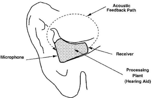
(14) The echo noise is acoustics feedback noise from oneself receiver to the microphone. We show the echo noise interference path in Fig. 2 [2] as follows.. Fig 2.. Acoustic feedback in a hearing aid inside of a human ear. The aforementioned issues motivate us to develop an echo canceller with low power consumption. For that reason, this thesis will focus on the low power design of echo canceller in hearing aids.. 1.2 Background of low power AEC design in hearing aids In this section, our background and basis will be presented here. First of all, we start to introduce overview of AEC (Acoustics Echo Cancellation) in hearing aids. Following section 2.1, section 2.2 will begin to introduce related works to you. 2.

(15) 1.2.1 Overview of AEC in hearing aids In section 1.2.1, three parts are included. 1. Types of hearing aids. 2. Echo canceller introduced in hearing aids. 3. LMS algorithm.. 1. Types of hearing aids For the appearance, we have four types of hearing aids [3]. ¾ ¾ ¾ ¾. Body type Eyeglass type Behind-the-Ear type(BTE) In-the-Ear type(ITE). Different types of hearing aids have different acoustic feedback. If hearing aids have no interference of the echo noise, the acoustic feedback canceller will not be needed anymore. Based on that, the appearance of hearing aids is very important to this thesis. Now that we introduce four types of hearing aids as follows:. Body type: The body type of hearing aids is shown in Fig. 3.. 3.

(16) Fig 3.. Body type of hearing aids. The body type shows us that the microphone, Processor and battery are not in the ear. Only the receiver is into the user’s ear. In this structure, acoustic feedback noise will not exist. Because of the path from receiver to microphone is too long, the echo noise effect is too weak. Nevertheless, this type is not convenience to use. This structure is too huge for user’s view. By this reason we know, we will go on next type right now, the eyeglass type.. Eyeglass type: The eyeglass type of hearing aids is shown in Fig. 4.. 4.

(17) Fig 4.. Eyeglass type of hearing aids. The eyeglass type shows us that microphone, receiver, Processor, and battery are all on the glasses. In this structure, acoustic feedback noise will not exist. That is because the path from receiver to microphone is too long. For that reason, the echo noise effect is weak too. This type is also not convenience to use.. Users will feel glasses too heavy to carry. People like smaller type as below, the behind-the-ear type and the in-the-ear type.. Behind-the-Ear type: The behind-the-ear type of hearing aids is shown in Fig. 5.. 5.

(18) Fig 5.. behind-the-ear type of hearing aids. The BTE type shows us that microphone, processor and battery are all behind the ear and only receiver will be in the ear. In this structure, acoustic feedback noise will begin to exist; the path from the receiver to the microphone is quite near, but echo noise effect is not very serious. In-the-ear type is the type we considered in this thesis. We will introduce this type in next page.. In-the-Ear type: In-the-ear type is shown in Fig. 6.. 6.

(19) Fig 6.. in-the-ear type of hearing aids. In-the-ear type shows us that microphone, processor, battery and receiver are all in the ear. That will be smaller, more convenience and more pleasing to appearance, but will have a very serious echo noise to interference user’s ear. ITE (in-the-ear) hearing aid needed echo canceller to eliminate the noise from its own receiver. In this thesis, we assume our hearing aids will be ITE hearing aids. Therefore, the echo noise feedback path will exist.. 2. Echo canceller introduced in hearing aids Fig. 7 show the diagram of hearing aids system to introduce the echo canceller [4].. 7.

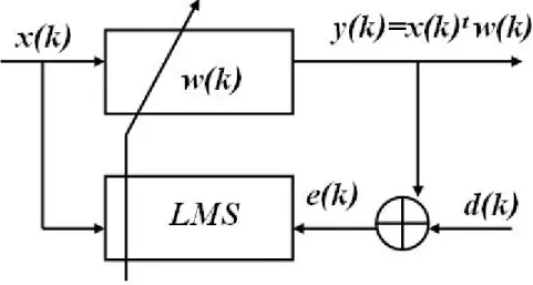
(20) Fig 7.. Diagram of hearing aids system. For hearing aids, the echo feedback noise is not welcomed. For that reason, we want to “filter” the echo noise. Besides, the echo channel is changed with time. Therefore, the filter is needed the characteristic of “adaptive”. Thus, the echo canceller is an adaptive filter [5]. Since our main issue is low power design for echo canceller, not all adaptive filter algorithms will be introduced. Other algorithms like NLMS [7], DLMS [8] will not be introduced in this thesis.. 3. LMS algorithm Fig 8 shows the diagram of LMS algorithm.. 8.

(21) Define: u: stepsize. (1.2.1). Fig 8.. d(k): desire signal e(k): error signal x(k): input signal vector w(k): window coefficient vector. Diagram of LMS algorithm. 1.2.2 Related works. In recent years, low-power designs for echo canceller in hearing aids usually focus on the architecture or circuit design. In this section, we will introduce those related work.. 9.

(22) 1.. Implementation of pipelined LMS adaptive filter for low-power VLSI applications [9].. The key idea of this design is using power minimization technique, likes Pipelining, Parallel Processing, and Relaxed Look Ahead to have lower frequency. For that reason, this filter can reduce the voltage, and power consumption. However, its problem is using pipelined LMS algorithm. That means 2 Multiplication for one operation of update & FIR part. Thus, its architecture complexity will be increased greatly (Large area, more switching activity for one operation). 2.. A Low power adaptive filter using dynamic reduced 2’s-complement representation [10].. This design proposed the use of a reduced 2’s complement signal representation to conditionally disable the internal signal transitions in the most-significant-bits of a data path. The key idea is to generate the signal representation dynamically according to the signal magnitude. The drawback of this approach is its high complexity due to LMS algorithm. It needs 2 Multiplication for one operation of update & FIR part. 3.. Ultra-low power DLMS adaptive filter for hearing aid applications[11].. This echo canceller presents an ultra-low-power, DLMS adaptive filter operating in the subthreshold region for hearing aid applications. In the architecture level, there are using a parallel architecture with pseudo nMOS (for leakage problem) logic style. The drawback of this approach is its high complexity due to DLMS algorithm.It needs 2 Multiplication for one operation of update & FIR part.. 10.

(23) 1.3 Thesis Organization First, we start to focus on our new P2SPT (Partial & Progressive Signed Power-of-Two) algorithm in Chapter 2. After demonstrating the P2SPT algorithm, we construct the acoustic feedback model to analyze and verify this new update algorithm’s performance. Therefore, we will introduce this model and show the Simulated Results in chapter 3. Then, in chapter 4, architecture designs and power reports will be presented. In the end, conclusion and future work will be given in Chapter 5.. 11.

(24) Chapter 2 Partial & Progressive Signed Power-of-Two (P2SPT) Algorithm Developing In this chapter, we will introduce the Partial & Progressive Signed Power-of-Two (P2SPT) algorithm. This algorithm is developed for simplest hardware complexity of echo canceller. The low hardware complexity will give us the low internal signal transition and the low area cost. With those two benefits, we will achieve our goal of low power. P2SPT algorithm is assembled by basic LMS algorithm, Sign-Sign algorithm [13], Power-of-Two window coefficient algorithm [14], 2-Staged Periodic Partial Update algorithm [15] and Progressive Update algorithm. We will introduce those algorithms in section 2.1 Background of P2SPT Algorithm. After section 2.1, we also have the clearly description in our P2SPT algorithm in section 2.2.. 2.1 Background of P2SPT Algorithm The well-know LMS algorithm is introduced in chapter 1. For that reason, we only describe others algorithms one by one in this section. Algorithms as follows: ¾ ¾ ¾ ¾. (2.1.1) Sign-Sign algorithm. (2.1.2) Power-of-Two window coefficient algorithm. (2.1.3) 2-Staged Periodic Partial Update algorithm. (2.1.4) Progressive Update algorithm.. 2.1.1 Sign-Sign Algorithm The computational complexity of the LMS algorithm is mainly due to multiplications performed in the coefficient updating and in the calculation of 12.

(25) the adaptive filter output. Because we want to minimize hardware complexity, the multiplications of the calculation have to be reduced. In this section, we focus on the hardware complexity of updating function part. We use the Sign-Sign algorithm to design the simplest updating function part. The coefficient updating in sign-sign algorithm is given by:. (2.1.4) The Sign-sign algorithm is the limit of quantized-data algorithm. We will have the simplest updating hardware cost, if we choose to use this algorithm. In function (2.1.4), we using function sgn(b) to change our two inputs. But only considering the Sign-sign algorithm will have the speed problem for updating function part. For example, the every one iteration will give us one Progressive unit step. Therefore, we will need last 1000 times iteration, if our updating coefficient is form 0 to 1000. For this reason, we will need the Progressive Update algorithm to improve speed of our echo canceller.. 2.1.2 Power-of-Two window coefficient algorithm It is well known that the complexity of a digital filter can be reduced by expressing its coefficients as sums of powers-of-two* (PT) terms [18]. The resulting filter requires no multiplier for coefficient multiplications and enjoys a saving in silicon area when implemented in VLSI [19]. Considering our requirement, we will have to use the Power-of-Two window coefficient algorithm in our echo canceller. Parameter vector defined and Power-of-Two window coefficient algorithm as shows as follows:. (2.1.8). (2.1.9). 13.

(26) for j:1…l. (2.1.10). (2.1.11) Where w(k+1) is as same as LMS algorithm defined, the base vector and the update vector are parameter vector by user’s requirement. We can unfold the function (2.1.10) to illustrate the base we defined.. (2.1.12) Following function (2.1.12), we can define the “base” is 2-base (i). For example, we will have three bases to use, if we choose the parameter b is equal to three. In Fig. 9, we assume there have 4 bases 2-3, 2-5, 2-7 and 2-9, and our update parameter only allows 0, 1, 2, and 4 to drive bases form all 0 to all 4. In this case, we can show all window coefficients in Fig. 9.. 0.7. 0.6. 0.5. 0.4. 0.3. 0.2. 0.1. 0. 0. 50. Fig 9.. 100. 150. 200. power of two window coefficient. 14. 250. 300.

(27) Using Power-of-Two to design the FIR part will lose coefficients precision and those coefficients will be nonlinear. Therefore, we must carefully to choose the “base” in Power-of-Two window coefficient algorithm.. 2.1.3 2-Staged Periodic Partial Update algorithm description Partial updating of the LMS adaptive filter has been proposed to reduce computational costs and power consumption [23]. For this reason, the partial update will be a part of our updating function. Our 2-Staged Periodic Partial Update algorithm is based on the Periodic partial update LMS algorithm [24] [25] [26]. Therefore, we will introduce this algorithm as follows.. 1. Periodic partial update LMS algorithm The most prevalent type in the literature of selective update scheme is referred to as the periodic partial update LMS algorithm. To reduce computation needed during the update part of the adaptive filter by a factor of N, the periodic partial update LMS algorithm updates all the filter coefficients every N iterations instead of every iteration. In addition, the coefficient updates for this algorithm are regular, as only one coefficient is changed at one iteration. With this concept, the coefficient update is given by:. (2.1.13). Where ⎣⎢⋅⎥⎦ denotes the truncation operation, k mod N denotes iteration k. 15.

(28) modulo N . By considering N iterations of the updates in function (2.1.13), it can be shown that this algorithm is equivalent to the following N-fold coefficient vector update:. (2.1.14) It describes a modified version of the LMS adaptive algorithm that uses every N-th instantaneous gradient to update the filter coefficients.. 2. 2-Staged Periodic partial update LMS algorithm Following Periodic partial update LMS algorithm, the 2-Staged Periodic partial update LMS algorithm is proposed. In fact, we just try to add one condition to change the update period of partial update. The 2-staged periodic partial update LMS algorithm as shows as follows:. (2.1.15). (2.1.16) In consequence, we double the period of partial update when our condition will be true. We use this 2-stage to control the partial update frequency. Therefore, we can have high frequency update when we have to match the echo channel, and have low update frequency if there are not necessary for our echo canceller.. 2.1.4 Progressive Update algorithm description. 16.

(29) Following section 2.1.1 to section 2.1.3, we can figure out the sign-sign algorithm means our update trigger will use the sign of input vector and the sign of error signal, the power-of-two window coefficient algorithm told us which the window coefficients only support power-of-two coefficients in the FIR part. In addition, we have 2-staged partial updating to reduce the computational cost. Besides, the most important part we are not discussed. Our encoder, it is to receive the update information and to transform this information to real window coefficients that we just need. Consequently, the encoder needs to have simplest hardware cost and also have enough updating speed to catch echo noise. Considering this two reason, we present this Progressive Update algorithm here. The Progressive Update algorithm as shows as follows:. (2.1.17). (2.1.18) We define the parameter coeff is a coefficient for this example. Next, we encode this parameter to produce the Vector p of b elements. Finally, we use those elements in the vector p to drive the “base” of FIR part. The example as shows follows:. (2.1.19) In section 2.2, we propose P2SPT algorithm after those basic algorithms integration.. 2.2 P2SPT Algorithm description. 17.

(30) In this thesis, we use the Partial & Progressive Signed Power-of-Two (P SPT) algorithm to design our echo canceller. Therefore, we present this algorithm here. First of all, we will define parameters for this algorithm. What is more, functions in this algorithm will be introduced on next page. Moreover, we will describe our P2SPT algorithm to you in the end. In the first, parameters and vectors as defines as follows: 2. 18.

(31) Bound function is shown as follows. We will use this function to limit the counter coefficient vector for our hardware design.. (2.2.1). Sign function is shown as follows; this function will be defined to process the vector X.. (2.2.2). Binary function is shown as follows; we have to define this function for care about the zero-state occurred.. (2.2.3). Partial function is shown as follows; the update trigger will impact our window coefficients when the partial function is allowed.. (2.2.4). 19.

(32) Following parameters and functions we defined, the P2SPT algorithm is presented here. Just like the traditional LMS algorithm, function (2.2.5) and (2.2.6) will produce the error signal en.. (2.2.5). (2.2.6. Than, we fresh and decompose our counter coefficient vector cn.. (2.2.7. (2.2.8). We will have new window coefficients in next iteration, when the updated operation is finished by the progressive coefficient matrix P(k,i) drive the base.. (2.2.9). Considering our Architecture design, we support window coefficients as shows as Fig. 11 P2SPT algorithm window coefficients in next page.. 20.

(33) In Fig. 10, we have 3 bases, and our update parameter only allows 0, 1, 2, and 4 to drive our bases form all 0 to all 4. In this case, window coefficients will be showed in Fig. 10.. 0.6. 0.4. 0.2. 0. -0.2. -0.4. -0.6. -60. -40. Fig 10.. -20. 0. 20. 40. 60. P2SPT algorithm window coefficients P. In order to have the minimum power consumption of echo canceller, we have developed this algorithm to obtain our goal of simplest architecture cost. In next chapter Acoustic Feedback Model Construction & Simulated Results, we will introduce the acoustic feedback model and simulate this algorithm to verify its performance. Accordingly, we will prove our algorithm’s performance as same as others, and based on our algorithm we can construct to simplest architecture.. 21.

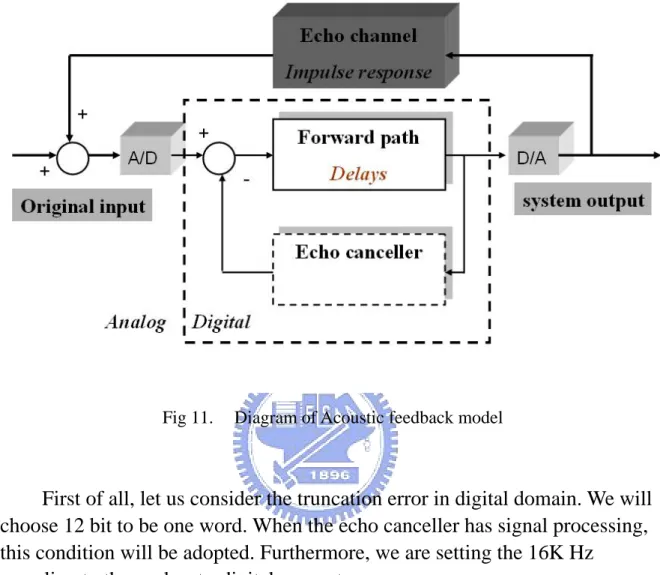
(34) Chapter 3 Acoustic Feedback Model Construction & Simulated Results In chapter 3 we will build a system model for realized acoustic feedback characteristics and help us to adjust the design of echo canceller. Moreover, we will also verify our P2SPT algorithm’s performance by this model. In section 3.1, we will start to construct our acoustic feedback model. For explain the operation of our model, a simple example will be presented in the end of this section. Following section 3.1, the section 3.2 will shows the simulated results for you.. 3.1 Model Construction. We will present section 3.1.1 model introduction to introduce our acoustic feedback model. Accordingly section 3.1.1, the example for model operation is showed in section 3.1.2.. 3.1.1 Model introduction Our model can be separated out of three parts in Fig. 12; the echo channel, the forward path and the echo canceller. There also have a two domain need to consider, the analog domain and the digital domain. We describe this model in next page.. We show Fig. 11 Diagram of Acoustic feedback model as follows.. 22.

(35) Fig 11.. Diagram of Acoustic feedback model. First of all, let us consider the truncation error in digital domain. We will choose 12 bit to be one word. When the echo canceller has signal processing, this condition will be adopted. Furthermore, we are setting the 16K Hz sampling to the analog-to-digital converter.. In Fig. 11, the model we built is including three parts. 1. Echo channel. 2. Forward path. 3. Echo canceller.. Now let us give a clear explanation for those three main parts as follows.. 1. Echo channel 23.

(36) According 1.2.1 Overview of AEC in hearing aids, we know ITE hearing aids will have echo noise exist. Therefore, we show the path of acoustic feedback in Fig. 12 [2].. Fig 12.. acoustic feedback path in the ear. In Fig. 12, we can find out the feedback channel. In consequence, the acoustic feedback channel means all the noise come from the receiver. For this reason, we can say “the path” is a response from the receiver’s signal. The acoustic feedback channel modeling [27] [28] [29], usually using the dummy head to describe the characteristic of echo path. For example, we according to the data form [30] and show you how to catch the characteristic of acoustic feedback path. First of all, the testing platform of dummy head will be setup already. Than, using the Sweep Stimulus method and the White Noise method to trigger the echo channel. Actually, we can also to say that it is tried to find out the impulse response in the time domain or the frequency response in the frequency domain. We show testing platform of the dummy head in Fig. 13.. 24.

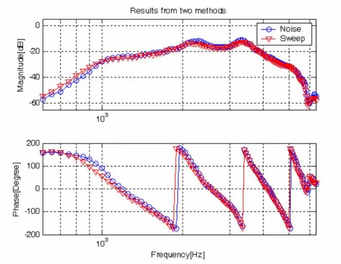
(37) Fig 13.. testing platform of dummy head. Legend for Fig. 13: (1) B&K head and torso simulator type 4128C (2) B&K right ear simulator type 4158C (3) Pinna simulator (4) ITE hearing instrument shell with a microphone and receiver (5) Knowles EA-1843 microphone (6) Knowles BK-1604 receiver (7) Acoustical feedback path (8) Interface between microphone and ADC (9) Interface between DAC and receiver (10) EZ-KIT LITE ADSP 2189M Evaluation Board, including a codec AD73322 and a DSP 2189. Based on this platform, we can describe the frequency response of Acoustic feedback channel like Fig. 14. 25.

(38) Fig 14.. frequency response of Acoustic feedback channel. In Fig. 14, there means Sweep Stimulus method and White Noise method will have the same result. We can find out the similarly response. According to this result, we can identity frequency response of acoustic feedback channel is just like Fig. 14. We can describe frequency response of our echo channel in Fig. 16. We show frequency response of our echo channel in Fig. 15.. 26.

(39) magnitude -10 -15 -20. dB. -25 -30 -35 -40 -45 -50. 3. 10. freq, Hz phase 4 3. radians. 2 1 0 -1 -2 -3. 3. 10. freq, Hz. Fig 15.. frequency response of our echo channel. In order to simulate echo noise effect, we need to do “convolution”. When system output signal feedback to microphone by echo path, the real echo noise is the convolution by output signal and echo channel. In a word, we will simulate our model in time domain. Consequently, we will need this echo channel impulse response.The echo channel will be changed to the 100 taps Finite Impulse Response (FIR). The result is on Fig. 16. Fig. 16 shows the Finite-Impulse-Response (FIR) of our model’s echo channel.. 27.

(40) 0.03. 0.02. 0.01. 0. -0.01. -0.02. -0.03. 0. 10. 20. 30. Fig 16.. 40. 50. 60. 70. 80. 90. 100. FIR of our echo channel. On other hand, the real echo feedback path is not steady. It will change with time. According to information from [31], we can list some characteristics for the echo feedback path in next page. The variation is depending on user’s physiological structure of ear and head in the feedback path of ITE hearing aids. Fig.17 will show the ear is a complicated structure.. 28.

(41) Fig 17.. Sketch of human ears. According to data we know, the variation statistics in the feedback path as shows as follows: ¾ The feedback path will have a ten percent of variation in the amplitude. ¾ The feedback path will change of 3~5ms.. Consider the variation of feedback echo path. We assume our echo channel will be changed by every 5ms, and the value of echo will have 10% variation with gauss random probability. Moreover, we also have two iteration delays variation of the echo channel with gauss random probability.. 2. Forward path This part is to simulate other function of hearing aids. In fact, forward path will include like compression part and band filters. But in this thesis, we only consider the effect of echo canceller. Therefore, we will use delays to 29.

(42) replace all functions in the forward path. In another word, the forward path just delays the input signal. This result will let us easy to know the performance of echo canceller by Mean-Square-Error (MSE) or human’s ear verification. Besides, the forward path delays we choose are 50 iteration delays. Fig. 18 shows Diagram of forward path.. Fig 18.. Diagram of forward path. 3. Echo canceller Echo canceller part can be any echo canceller we like, if the echo canceller is adaptive filter form. Therefore, we draw the diagram of dotted line. Furthermore, we will use a basic adaptive echo canceller (LMS filter) to show our model’s operation, and use our algorithm to prove the performance in section 3.2. Fig. 19 shows Diagram of echo canceller.. Fig 19.. Diagram of echo canceller. 3.1.2 Example for Model’s Operation We will describe our model’s operation by an example. The model will be introduced in section 3.1.1. Therefore, the echo canceller is a LMS filter and work on the 12 bits and 16 KHz sampling rate. 30.

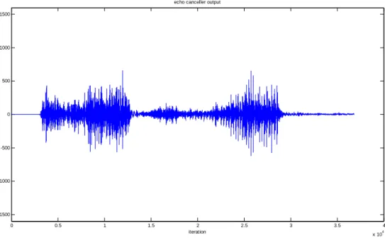
(43) First of all, we assume that the original signal is like Fig. 20. The Y-axis is from -0.8 to 0.8 and X-axis from 0 to 40000 (unit: iterations). This signal is the voice by man. The signal length as longs as one second. original input 0.8. 0.6. 0.4. 0.2. 0. -0.2. -0.4. -0.6. -0.8. 0. 0.5. 1. Fig 20.. 1.5. 2 iteration. 2.5. 3. 3.5. 4 4. x 10. Waveform of the original signal. This operation of our model is input this original signal into the forward path, there means delay by 50 iterations than the signal will output to be the system output. In consequence, this system output will start feedback to interfere original signal by echo path. Furthermore, the echo canceller will use this system output to make the echo canceller’s output. Those results will show in the Fig. 21 Waveform of the echo canceller output signal and Fig. 22Waveform of the system output signal.. Fig. 21 shows us the echo canceller output signal.. 31.

(44) echo canceller output 1500. 1000. 500. 0. -500. -1000. -1500 0. 0.5. 1. Fig 21.. 1.5. 2 iteration. 2.5. 3. 3.5. 4 4. x 10. Waveform of the echo canceller output signal. In Fig. 22, the system output signal with echo canceller is presented. Because echo canceller’s output will cancel real echo noise in our model, this output signal is to be similar with original voice. system output 0.8. 0.6. 0.4. 0.2. 0. -0.2. -0.4. -0.6. -0.8. 0. 0.5. 1. Fig 22.. 1.5. 2 iteration. 2.5. 3. 3.5. 4 4. x 10. Waveform of the system output signal. Now, if we turn off this echo canceller. The system output will be look 32.

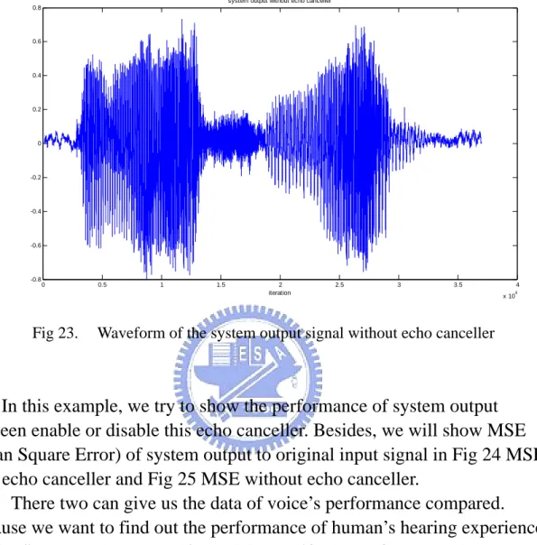
(45) like Fig. 23. In this case, the sound of this signal will bring a bleep that we called echo noise. system output without echo canceller 0.8. 0.6. 0.4. 0.2. 0. -0.2. -0.4. -0.6. -0.8. 0. Fig 23.. 0.5. 1. 1.5. 2 iteration. 2.5. 3. 3.5. 4 4. x 10. Waveform of the system output signal without echo canceller. In this example, we try to show the performance of system output between enable or disable this echo canceller. Besides, we will show MSE (Mean Square Error) of system output to original input signal in Fig 24 MSE with echo canceller and Fig 25 MSE without echo canceller. There two can give us the data of voice’s performance compared. Because we want to find out the performance of human’s hearing experience, not the filter speed. We use this model to verify the performance that we want to know like this example. Consequently, we will use the same data like this example to show you that our algorithm’s performance and others in next section. Moreover, we will show the (Signal Noise Ratio) SNR and the voice’s Spectrogram to prove that our algorithm has the same performance to other LMS-based algorithms.Fig 24 shows the MSE (with echo canceller) of system output to original input.. 33.

(46) MSE. 0.2. 0.15. 0.1. 0.05. 0. 0. Fig 24.. 0.5. 1. 1.5. 2 iteration. 2.5. 3. 3.5. 4 4. x 10. MSE (with echo canceller) of system output to original input. Fig 25 shows the MSE (without echo canceller) of system output to original input. We can see the difference between Fig. 24 and Fig. 25, if we try to compare these two figures. MSE without echo canceller. 0.2. 0.15. 0.1. 0.05. 0. 0. Fig 25.. 0.5. 1. 1.5. 2 iteration. 2.5. 3. 3.5. 4. MSE (without echo canceller) of system output to original input. 34. 4. x 10.

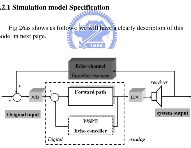
(47) 3.2 Simulated Results In this section, we will simulate our P2SPT algorithm on the MATLAB. According to section 3.1, our model’s Specification will be ordered in section 3.2.1. In section 3.2.2, we will compare our algorithm with other well-know LMS-based algorithms. In section 3.2.3, we will show the performance on human’s voice test. We will poof our algorithm has good performance as same as other algorithms in the performance of echo cancellation. Besides, we will have simplest architecture in our hardware design that we need.. 3.2.1 Simulation model Specification Fig 26as shows as follows; we will have a clearly description of this model in next page.. Fig 26.. model of simulation. 35.

(48) In Fig 26, we will have two domain and four main units in our model. First, we define sample rate will be 16 KHz, as same as our hardware specification. In the next, we start to discuss those two domains. Our design will work on the digital domain. Therefore, we will have the truncation error problem that we have to consider about. In addition, the unwelcome really echo noise is an analog signal. Considering this reason, when the signal is processed in the digital domain we will transform our signal to 12 bit precision. Considering four main units in Fig 26, we describe the forward path first. In reality, the forward path means the compression and other functions in the hearing aid. But we are only considering the echo cancellation in this thesis. For this reason, we just assume our forward path is 50 iteration delays. In the echo canceller unit, we design this echo canceller using the P2SPT algorithm. Moreover, we describe this unit as same as our hardware design. In consequence, we can verify our hardware design of compared the output signal for this simulation model and our real design. Echo channel is a matrix. This matrix saves the echo impulse response which introduced in section 3.1. Furthermore, we change this channel with every 3ms on the variation condition that also introduced in section 3.1 too. In the last part, the receiver effect will be considered. In practice, our receiver will amplify the system output. Accordingly, we have to assume the worst case in our echo model. We will have to amplify our system output to 12db.In next page, we form that information of this model in table 1 information of simulation model.. Table 1 information of simulation model shows simulation model’s information as follows: table 1.. information of simulation model. Specification. Description.. Digital sample rate. 16K (Hz). Digital Bit number. 12 (bit). forward path. 50 delays (iterations) 36.

(49) Echo canceller Echo channel. P2SPT ( using our algorithm) Also can change to other algorithms. Matrix (1x100) Channel change every 3ms. (Variation with Gauss random) 90% ~ 110% of amplitude. -1 and 1 delay iteration will plus to channel.. Receiver effect. Our system output Amplify to 12db.. In next section, we will start compare our algorithm with other well-know LMS based algorithms in this model. Actually, we are not proved that our algorithm is faster or more accurately than others. The result we want to show you that is our algorithm has the same performance in human’s hearing experience. As we can know, our user will feel nothing of echo noise when they wear the hearing aid, if the feedback echo noise is under the allowed range [32]. For that reason, we can have the simplest hardware design for low power issue and our user also not interfere by echo noise.. 3.2.2 Algorithms compared In this section, we will prove our algorithm’s performance will be as same as other algorithm’s performance in echo cancellation of the model we introduced in section 3.2.1. In Fig. 27 learning curves of four algorithms, we will show the LMS, DLMS, NLMS and our P2SPT algorithm’s learning curve.. 37.

(50) Learning Cruve 0.08 P2SPT NLMS DLMS LMS. 0.07. 0.06. MSE (linear scale). 0.05. 0.04. 0.03. 0.02. 0.01. 0. 200. 400. 600. Fig 27.. 800. 1000 1200 number of iterations. 1400. 1600. 1800. 2000. learning curves of four algorithms. Our input signal is a random white noise signal between 1 and -1. Moreover, we also put in 10% noise to the input signal. All algorithms will have 32 taps and LMS algorithm’s step-size is 0.1, DLMS algorithm’s step-size is 0.1 too. Considering the model we built, the channel of we learning is the echo channel that we introduced in section 3.1. in Fig 27, if we compare speed of these algorithms, we have the order from fast to slow will be: NLMS > P2SPT > LMS > DLMS.. If we compare precision of these algorithms, we can find out the order from batter to bad precision will be: NLMS > LMS > DLMS > P2SPT.. In fact, we want to compare the performance of “echo canceller’s algorithms”, not the filter speed or precision. Therefore, we will use the model (introduced in section 3.2.1) to verify all of algorithm’s performance of echo cancellation. 38.

(51) Consequently, to compare the speed or the precision of those filters can not really find out the result we want. Only to compare those algorithms by real voice’s signal and have real echo noise occurred, the result will mean real performance of echo cancellation. First of all, we will show the LMS algorithm. Next, we will have the DLMS algorithm and the NLMS algorithm. Finally, we will show our P2SPT algorithm’s performance and the performance of not using echo canceller to you.. LMS algorithm: In next page, we will have the information of four types in Fig 29 LMS algorithm’s performance. We have the original input signal in lower left-hand corner, and system output in lower right-hand corner. In upper left, we have the echo canceller output. In upper right, we show the MSE of original input and system output. Accordingly, Fig. 29 Fig 30, Fig. 31 and Fig. 32 are following this order. Besides, we will show the MSE result of those algorithms in the end. Fig. 28 as shows as follows: echo canceller output. Mean squared error for system output & original input. 3000. 0.07. 2000. 0.06 0.05. 1000. 0.04 0 0.03 -1000. 0.02. -2000 -3000. 0.01. 0. 0.5. 1. 1.5. 2. 2.5. 3. 3.5. 0. 4. 0. 0.5. 1. 1.5. 2. 2.5. 3. 3.5. 4. x 10. original input. system output. 0.6. 0.6. 0.4. 0.4. 0.2. 0.2. 0. 0. -0.2. -0.2. -0.4. -0.4. -0.6. -0.6. -0.8. 0. 0.5. 1. 1.5. 2. 4 4. x 10. 2.5. 3. 3.5. -0.8. 4. 0. 0.5. 1. 1.5. 4. Fig 28.. 2. 2.5. 3. 3.5. 4 4. x 10. x 10. LMS algorithm’s performance. 39.

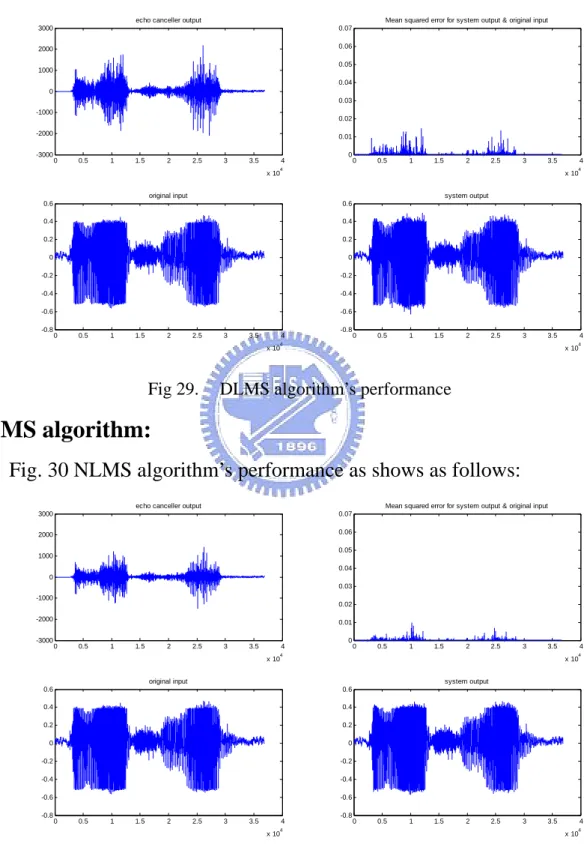
(52) DLMS algorithm: Fig. 29 as shows as follows, our delay parameter is four iterations. echo canceller output. Mean squared error for system output & original input. 3000. 0.07. 2000. 0.06 0.05. 1000. 0.04 0 0.03 -1000. 0.02. -2000 -3000. 0.01. 0. 0.5. 1. 1.5. 2. 2.5. 3. 3.5. 0. 4. 0. 0.5. 1. 1.5. 2. 2.5. 3. 3.5. 4. x 10. original input. system output. 0.6. 0.6. 0.4. 0.4. 0.2. 0.2. 0. 0. -0.2. -0.2. -0.4. -0.4. -0.6. -0.6. -0.8. 0. 0.5. 1. 1.5. 2. 4 4. x 10. 2.5. 3. 3.5. -0.8. 4. 0. 0.5. 1. 1.5. 2. 2.5. 3. 3.5. 4. Fig 29.. 4 4. x 10. x 10. DLMS algorithm’s performance. NLMS algorithm: Fig. 30 NLMS algorithm’s performance as shows as follows: echo canceller output. Mean squared error for system output & original input. 3000. 0.07. 2000. 0.06 0.05. 1000. 0.04 0 0.03 -1000. 0.02. -2000 -3000. 0.01. 0. 0.5. 1. 1.5. 2. 2.5. 3. 3.5. 0. 4. 0. 0.5. 1. 1.5. 2. 2.5. 3. 3.5. 4. x 10. original input. system output. 0.6. 0.6. 0.4. 0.4. 0.2. 0.2. 0. 0. -0.2. -0.2. -0.4. -0.4. -0.6. -0.6. -0.8. 0. 0.5. 1. 1.5. 2. 4 4. x 10. 2.5. 3. 3.5. -0.8. 4. 0. 0.5. 1. 1.5. 4. Fig 30.. 2. 2.5. 3. 3.5. 4 4. x 10. x 10. NLMS algorithm’s performance. 40.

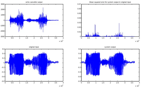
(53) P2SPT algorithm: P. Fig. 31 P2SPT algorithm’s performance as shows as follows: echo canceller output. Mean squared error for system output & original input. 3000. 0.07. 2000. 0.06 0.05. 1000. 0.04 0 0.03 -1000. 0.02. -2000 -3000. 0.01. 0. 0.5. 1. 1.5. 2. 2.5. 3. 3.5. 0. 4. 0. 0.5. 1. 1.5. 2. 2.5. 3. 3.5. 4. x 10. original input. system output. 0.6. 0.6. 0.4. 0.4. 0.2. 0.2. 0. 0. -0.2. -0.2. -0.4. -0.4. -0.6. -0.6. -0.8. 0. 0.5. 1. 1.5. 2. 4 4. x 10. 2.5. 3. 3.5. -0.8. 4. 0. 0.5. 1. 1.5. 2. 2.5. 3. 3.5. 4. Fig 31.. 4 4. x 10. x 10. P2SPT algorithm’s performance. Using no echo canceller: Fig. 32 no echo canceller’s performance as shows as follows: echo canceller output. Mean squared error for system output & original input. 3000. 0.07. 2000. 0.06 0.05. 1000. 0.04 0 0.03 -1000. 0.02. -2000 -3000. 0.01. 0. 0.5. 1. 1.5. 2. 2.5. 3. 3.5. 0. 4. 0. 0.5. 1. 1.5. 2. 2.5. 3. 3.5. 4. x 10. original input. system output. 0.6. 0.6. 0.4. 0.4. 0.2. 0.2. 0. 0. -0.2. -0.2. -0.4. -0.4. -0.6. -0.6. -0.8. 0. 0.5. 1. 1.5. 2. 4 4. x 10. 2.5. 3. 3.5. -0.8. 4. 0. 0.5. 1. 1.5. 4. Fig 32.. 2. 2.5. 3. 3.5. 4 4. x 10. x 10. no echo canceller’s performance. 41.

(54) We use table 2 MSE of algorithms to show the performance of those algorithms. table 2.. the performance of algorithms. Algorithm Type. NLMS. LMS. DLMS. P2SPT. Using NO canceller. MSE (unit: 10^-4) SNR (db). 0.2297. 0.421. 0.4174. 1.93. 13.36. 32.79. 30.16. 30.19. 23.55. 15.14. P. Our algorithm’s performance look likes not better than others. But in the users hear, all of algorithms can cancel the echo except using no echo canceller. In fact, human’s hearing feel nothing when the echo noise under the allowed range [32]. We will use the spectrogram graphs to prove this point in next page.. Spectrograms comparison: We have the original input wave in upper left-hand corner, and the spectrograms of original input in upper right -hand corner. In lower left, we have the spectrograms of system output without echo canceller. In lower right, we show the spectrograms of P2SPT system output. Fig. 33 as shows as follows:. 42.

(55) Fig 33.. (a) original input wave. The spectrograms of (b) original input (c) system output without echo canceller (d) P2SPT system output. To compare with original input, we can find out the different between system output without echo canceller and P2SPT system output. The high frequency energy occurs in system output without echo canceller. We will compare our P2SPT system output with others in next page. Therefore, we can analyze those spectrograms plots to prove there no different in user’s experience. We have the spectrograms of NLMS system output in upper left-hand corner, and the spectrograms of LMS system output in upper right -hand corner. In lower left, we have the spectrograms of DLMS system output. In lower right, we show the spectrograms of P2SPT system output. Fig. 34 as shows as follows:. 43.

(56) Fig 34.. The spectrograms of (a) NLMS system output (b) LMS system output (c) DLMS system output (d) P2SPT system output. In Fig. 34, there are not evidence that our algorithm’s performance is bad than others. In fact, our algorithm only increases a little bit high frequency energy and there are not occur any effect in user’s hearing experience.. 3.2.3 Performance on human’s voice In this section, we will show you that our algorithm has good echo cancellation performance in human’s voice input. In consequence, we will use the same model to verify algorithm’s performance on human’s voice testing. In fact, all we really want is reduced the power consumption of echo canceller. Therefore, to compare the speed or the precision is not the point we considered. For that reason, we only to show you that the echo noise will be eliminated in spectrogram and waveform graphs. 44.

(57) First, we will show the test of 4 types human’s voice to you. Moreover, considering the testing of long voice’s stability and forward path changed, we will verify those two parts in the end.. In human’s voice testing, we present four voice’s types as follows: ¾ ¾ ¾ ¾. Man’s voice. Woman’s voice. Boy’s voice. Girl’s voice.. For those different types, we will show you that the echo cancellation performance of our P2SPT algorithm in spectrogram and waveform graphs. Accordingly, those four types will have different echo noise response. Consequently, Boy’s voice will be lowest frequency voice and woman’s voice is highest frequency voice in this test. Therefore, we can prove to you that our algorithm is real useful of echo cancellation in hearing aid.. Man’s voice: First of all, we assume that man’s original signal is like Fig. 35. The Y-axis is from -1 to 1 and X-axis from 0 to 12000 (unit: iterations).. 45.

(58) 1. 0.8. 0.6. 0.4. 0.2. 0. -0.2. -0.4. -0.6. -0.8. -1. 0. 2000. Fig 35.. 4000. 6000. 8000. 10000. 12000. Waveform of man’s original signal. In addition, we show echo canceller output in Fig. 36 Waveform of man’s echo canceller output signal. (12bit: value 2048 means 1). 2000. 1500. 1000. 500. 0. -500. -1000. -1500. -2000 0. 2000. Fig 36.. 4000. 6000. 8000. 10000. 12000. Waveform of man’s echo canceller output signal. Our system output will as shows as follows; under the echo canceller work.. 46.

(59) 1. 0.8. 0.6. 0.4. 0.2. 0. -0.2. -0.4. -0.6. -0.8. -1. 0. 2000. Fig 37.. 4000. 6000. 8000. 10000. 12000. Waveform of man’s system output signal. Now, if we turn off the echo canceller. The system output will be look like Fig. 38. In this case, the sound of this signal will bring a bleep that we call echo noise. (Y-axis also from -1 to 1). 1. 0.8. 0.6. 0.4. 0.2. 0. -0.2. -0.4. -0.6. -0.8. -1. Fig 38.. 0. 2000. 4000. 6000. 8000. 10000. 12000. Waveform of man’s system output signal without echo canceller. We will show MSE of system output to original input. Also, we will show MSE without echo canceller too. Fig. 39 shows MSE (with echo canceller) of 47.

(60) system output to original input. (Y-axis is from 0 to 2). 2. 1.8. 1.6. 1.4. 1.2. 1. 0.8. 0.6. 0.4. 0.2. 0. 0. 2000. Fig 39.. 4000. 6000. 8000. 10000. 12000. MSE (with echo canceller) of man’s testing. Fig. 40 shows MSE (without echo canceller) of system output to original input. (Y-axis is from 0 to 2). 2. 1.8. 1.6. 1.4. 1.2. 1. 0.8. 0.6. 0.4. 0.2. 0. 0. 2000. Fig 40.. 4000. 6000. 8000. 10000. 12000. MSE (without echo canceller) of man’s testing. Man’s spectrograms results as shows as follows. In Fig. 43, we can see the energy distribution is different with Fig. 41. On other hand, the 48.

(61) spectrograms result of Fig. 42 is similar to Fig. 41.. Fig 41.. Fig 42.. Fig 43.. Spectrograms of man’s original signal. Spectrograms of man’s system output signal. Spectrograms of man’s system output signal without echo canceller. 49.

(62) Woman’s voice: As same as man’s voice testing, woman’s original signal is like Fig. 44. The Y-axis is from -1 to 1 and X-axis from 0 to 18000 (unit: iterations).. 1. 0.8. 0.6. 0.4. 0.2. 0. -0.2. -0.4. -0.6. -0.8. -1. 0. 2000. 4000. Fig 44.. 6000. 8000. 10000. 12000. 14000. 16000. 18000. Waveform of woman’s original signal. Besides, we will show the echo canceller output in Fig. 45 Waveform of woman’s echo canceller output signal. (12bit: value 2048 means 1). 2000. 1500. 1000. 500. 0. -500. -1000. -1500. -2000 0. 2000. Fig 45.. 4000. 6000. 8000. 10000. 12000. 14000. 16000. Waveform of woman’s echo canceller output signal. 50. 18000.

(63) Our system output will as shows as follows; with echo canceller work.. 1. 0.8. 0.6. 0.4. 0.2. 0. -0.2. -0.4. -0.6. -0.8. -1. 0. 2000. Fig 46.. 4000. 6000. 8000. 10000. 12000. 14000. 16000. 18000. Waveform of woman’s system output signal. As well, we also turn off the echo canceller. The system output will be look like Fig. 47. (Y-axis also from -1 to 1). 1. 0.8. 0.6. 0.4. 0.2. 0. -0.2. -0.4. -0.6. -0.8. -1. Fig 47.. 0. 2000. 4000. 6000. 8000. 10000. 12000. 14000. 16000. 18000. Waveform of woman’s system output signal without echo canceller. 51.

(64) Fig. 48 shows MSE (with echo canceller) of system output to original input. (Y-axis is from 0 to 0.4). 0.4. 0.35. 0.3. 0.25. 0.2. 0.15. 0.1. 0.05. 0. 0. 2000. Fig 48.. 4000. 6000. 8000. 10000. 12000. 14000. 16000. 18000. MSE (with echo canceller) of woman’s testing. Fig. 49 shows MSE (without echo canceller) of system output to original input. (Y-axis is from 0 to 0.4). 0.4. 0.35. 0.3. 0.25. 0.2. 0.15. 0.1. 0.05. 0. 0. 2000. Fig 49.. 4000. 6000. 8000. 10000. 12000. 14000. 16000. MSE (without echo canceller) of woman’s testing. 52. 18000.

(65) Woman’s spectrograms results as shows as follows. In Fig. 52, we can see the energy distribution is also different with Fig. 50 and the spectrograms result of Fig. 51 is similar to Fig. 50.. Fig 50.. Fig 51.. Fig 52.. Spectrograms of woman’s original signal. Spectrograms of woman’s system output signal. Spectrograms of woman’s system output signal without echo canceller. 53.

(66) Boy’s voice: The boy’s original signal is like Fig. 53. The Y-axis is from -1 to 1 and X-axis from 0 to 20000 (unit: iterations).. 1. 0.8. 0.6. 0.4. 0.2. 0. -0.2. -0.4. -0.6. -0.8. -1. 0. 0.2. 0.4. 0.6. 0.8. 1. 1.2. 1.4. 1.6. 1.8. 2 4. x 10. Fig 53.. Waveform of boy’s original signal. We will show the echo canceller output in Fig. 54 Waveform of boy’s echo canceller output signal. (12bit: value 2048 means 1). 2000. 1500. 1000. 500. 0. -500. -1000. -1500. -2000 0. 0.2. 0.4. 0.6. 0.8. 1. 1.2. 1.4. 1.6. 1.8. 2 4. x 10. Fig 54.. Waveform of boy’s echo canceller output signal. 54.

(67) Our system output will as shows as follows; under the echo canceller work.. 1. 0.8. 0.6. 0.4. 0.2. 0. -0.2. -0.4. -0.6. -0.8. -1. 0. 0.2. 0.4. 0.6. 0.8. 1. 1.2. 1.4. 1.6. 1.8. 2 4. x 10. Fig 55.. Waveform of boy’s system output signal. In next graph, if we also turn off the echo canceller. The system output will be look like Fig. 56. (Y-axis also from -1 to 1). 1. 0.8. 0.6. 0.4. 0.2. 0. -0.2. -0.4. -0.6. -0.8. -1. 0. 0.2. 0.4. 0.6. 0.8. 1. 1.2. 1.4. 1.6. 1.8. 2 4. x 10. Fig 56.. Waveform of boy’s system output signal without echo canceller. 55.

(68) Fig. 57 shows MSE (with echo canceller) of system output to original input. (Y-axis is from 0 to 0.35). 0.3. 0.25. 0.2. 0.15. 0.1. 0.05. 0. 0. 0.2. 0.4. 0.6. 0.8. 1. 1.2. 1.4. 1.6. 1.8. 2 4. x 10. Fig 57.. MSE (with echo canceller) of boy’s testing. Fig 58shows MSE (without echo canceller) of system output to original input. (Y-axis is from 0 to 0.35). 0.35. 0.3. 0.25. 0.2. 0.15. 0.1. 0.05. 0. 0. 0.2. 0.4. 0.6. 0.8. 1. 1.2. 1.4. 1.6. 1.8. 2 4. x 10. Fig 58.. MSE (without echo canceller) of boy’s testing. 56.

(69) Boy’s spectrograms results as shows as follows. In Fig. 61, we can see the energy distribution is different with Fig. 59 and the spectrograms result of Fig. 60 is similar to Fig. 61.. Fig 59.. Fig 60.. Fig 61.. Spectrograms of boy’s original signal. Spectrograms of boy’s system output signal. Spectrograms of boy’s system output signal without echo canceller. 57.

(70) Girl’s voice: The girl’s original signal is like Fig. 62. The Y-axis is from -1 to 1 and X-axis from 0 to 15000 (unit: iterations).. 1. 0.8. 0.6. 0.4. 0.2. 0. -0.2. -0.4. -0.6. -0.8. -1. 0. 5000. Fig 62.. 10000. 15000. Waveform of girl’s original signal. The echo canceller output in Fig 63 Waveform of girl’s echo canceller output signal, as shows as follows. (12bit: value 2048 means 1). 2000. 1500. 1000. 500. 0. -500. -1000. -1500. -2000 0. 5000. Fig 63.. 10000. Waveform of girl’s echo canceller output signal. 58. 15000.

(71) Our system output will as shows as follows; under the echo canceller work.. 1. 0.8. 0.6. 0.4. 0.2. 0. -0.2. -0.4. -0.6. -0.8. -1. 0. 5000. Fig 64.. 10000. 15000. Waveform of girl’s system output signal. If we also turn off the echo canceller, the system output will be look like Fig. 65. (Y-axis also from -1 to 1). 1. 0.8. 0.6. 0.4. 0.2. 0. -0.2. -0.4. -0.6. -0.8. -1. 0. Fig 65.. 5000. 10000. 15000. Waveform of girl’s system output signal without echo canceller. 59.

(72) Fig. 66 shows MSE (with echo canceller) of system output to original input. (Y-axis is from 0 to 0.25). 0.25. 0.2. 0.15. 0.1. 0.05. 0. 0. 5000. Fig 66.. 10000. 15000. MSE (with echo canceller) of girl’s testing. Fig. 67 shows MSE (without echo canceller) of system output to original input. (Y-axis is from 0 to 0.25). 0.25. 0.2. 0.15. 0.1. 0.05. 0. 0. 5000. Fig 67.. 10000. MSE (without echo canceller) of girl’s testing. 60. 15000.

(73) Girl’s spectrograms results as shows as follows. In Fig. 70, we can see the energy distribution is different with Fig. 68 and the spectrograms result of Fig. 69 is similar to Fig. 68.. Fig 68.. Fig 69.. Fig 70.. Spectrograms of girl’s original signal. Spectrograms of girl’s system output signal. Spectrograms of girl’s system output signal without echo canceller. 61.

(74) We will form all MSE and SNR of voice test in table 4.3.1 MSE of voice testing. table 3.. MSE with Echo canceller MSE w/o Echo canceller SNR (db) with Echo canceller SNR (db) w/o Echo canceller. performance of voice testing. man 0.0026. woman 0.00058188. boy 0.0013. girl 0.00042373. 0.0422. .006. 0.0059. 0.0031. 18.43. 26.153. 17.78. 16.23. 6.334. 6.02. 11.21. 7.589. In table 3, we can discover our echo canceller can reduced the most echo noise in MSE and SNR data results. Moreover, we also use the spectrograms to prove our algorithm has good performance in echo cancellation result. Therefore, the echo noise will not influence our user’s hearing experience when our algorithm worked. In next topic, we will discuss that the long voice testing and forward path delays changed effect for our algorithm.. Forward path delays changed: We consider the forward path delays effect in this model. We will show you that the performance of echo cancellation is not depended on the forward path delays. We use MSE to show you that the performance of echo cancellation is not depended on the forward path delays in table 4 MSE of forward path delays changed. We use man’s voice signal as shows as follows. The result of table 4 is not depended on forward path iteration delays. Therefore, other components of hearing aid will have more design adaptability. 62.

(75) table 4.. Iteration delays MSE. MSE of forward path delays changed. 50. 100. 150. 300. 0.0026. 0.00255. 0.00252. 0.00264. Long voice’s testing: In order to test the stability of our algorithm, we use the voice’s signal of 700000 iterations (almost 44 seconds) to prove our algorithm will adaptive the window coefficient for control the echo noise. In Fig. 71 original long voice’s signal, we have the system input for our model.. 0.8. 0.6. 0.4. 0.2. 0. -0.2. -0.4. -0.6. -0.8. -1. 0. 1. 2. 3. 4. 5. 6. 7 5. x 10. Fig 71.. original long voice’s signal. In Fig. 72 long voice’s system output signal, we have the system output for our model.. 63.

(76) 0.8. 0.6. 0.4. 0.2. 0. -0.2. -0.4. -0.6. -0.8. -1. 0. 1. 2. 3. 4. 5. 6. 7 5. x 10. Fig 72.. long voice’s system output signal. In Fig. 72, we can find out the system output will sounds like the original input signal in the human’s hearing experience. Actually, the key point of this thesis is low power design. So we just achieved the goal of cancelled echo noise and will focus on real design’s power consumption. Accordingly, we just prove our algorithm is achieved the goal of cancelled echo noise in human’s hearing experience. Therefore, we will have the simplest architecture design when we using our P2SPT algorithm in next chapter, Chapter 4 Architecture Designs & Power Reports.. 64.