微聚焦端泵浦摻釹釩酸釔雷射在簡併共振腔下被修正過的自發輻射

國

立

交

通

大

學

光電工程研究所

碩

士

論

文

微聚焦端泵浦摻釹釩酸釔雷射在簡併共振腔下被修正

過的自發輻射

Modified Spontaneous Emission in a Tightly Pumped

Nd:YVO

4

Laser with Degenerate Resonator

研 究 生：邱偉豪

指導教授：謝文峰 教授

微聚焦端泵浦摻釹釩酸釔雷射在簡併共振腔下被修正

過的自發輻射

Modified Spontaneous Emission in a Tightly Pumped

Nd:YVO

4

Laser with Degenerate Resonator

研 究 生：邱偉豪

Student: Wei-Hao Chiu

指導教授：謝文峰 教授

Advisor: Dr. Wen-Feng Hsieh

國立交通大學

光電工程研究所

碩士論文

A Thesis

Aubmitted to Institute of Electro-Optical Engineering College of Electrical Engineering and

Computer Science National Chiao Tung University In Partial Fulfillment of the Requirements

for the Degree of Master

In

Electro-optical Engineering June 2005

Hsin-chu, Taiwan, Republic of China

i

微聚焦端泵浦摻釹釩酸釔雷射在簡併共振腔下被修正過的

自發輻射

研究生: 邱偉豪 指導教授: 謝文峰 教授

國立交通大學光電工程研究所

摘要

我們在小光束端泵浦摻釹釩酸釔雷射中觀察到不尋常的自發輻射行為。我們 在實驗上也證明了在簡併腔位置自發輻射的輸出功率會比非簡併腔位置高。從單 模速率方程式的定性分析，我們可以得到在簡併腔位置的β(自發輻射的耦合效 率)和 1/τf (1/τf 是自發輻射的衰減時間)比非簡併腔位置的值大。另外，我們也觀 察到了被修正過的自發輻射的場形。

ii

Modified Spontaneous Emission in a Tightly Pumped Nd:YVO

4

Laser with Degenerate Resonator

Student: Wei-Hao Chiu Advisor: Prof. Wen-Feng Hsieh

Institute of Electro-Optical Engineering

National Chaio Tung University

Abstract

The queer spontaneous emission behavior of an axially pumped Nd:YVO4 laser

is observed under a small pumping spot size. We experimentally demonstrate that the output power of spontaneous emission in degeneracy cavity is larger than in non-degeneracy cavity. From the qualitative analysis of single mode rate equation, we conclude β (the spontaneous emission coupling efficiency) and 1/τf (τf is the

spontaneous decay time) at degeneracy is larger than at non-degeneracy. In addition, we also observed modified spontaneous emission pattern.

iii

Acknowledgements

我常以為，學如逆水行舟，而今輕舟已過萬重山。一路行來，點滴在心，雖 然這不是一部完美的論文，但這部論文的完成，要感謝的真的人很多，僅以此文 表達我的誠摯謝意。 首先，在這短短的兩年之間，第一個要感謝的當然就是恩師-謝文峰教授， 不管是論文撰寫、研究態度與方法、為人處世各方面都花費心思，細心指導。藉 此，獻上最高的謝意。以及，東海大學物理系的吳小華教授對於我實驗上的建議。 還有，師出同門的雷射組學長們-家弘、陳慶緒學長、小戴、智章、史萊姆、阿 猴把我帶入了雷射的這個研究領域，並且在研究上幫了我很多的忙，使得這篇論 文可得以更加完整。 當然，在這兩年的生活，並不是只有實驗與研究而已。其它實驗室的的學長 姐，阿政、黃董，維仁(可以少抽一點菸了~)、晴如學姊、信民、楊松(股市會大 漲的~)、奎哥…也在生活上給了我建議，在這也祝福三位跟我一起畢業的學長-小戴、阿政以及奎哥一帆風順。另外，就是一起成長的同學了，阿笑姐、大頭峰、 華仔斌、阿勛和小毅，也很感謝他們的幫忙，讓我們一起成長、一起畢業。接下 來就是本實驗室最寶貝的唯一碩一學弟-阿榕，幫忙完成了許多實驗室的雜務以 及瑣事，在這裡也要感謝他。 當然，還有要在這感謝電資 401 共同實驗室提供實驗儀器，以及國科會 NSC 93-2112-M009-035 計劃的支持，讓我的實驗得以順利完成。 最後，我將這篇論文獻給我摯愛的父母。

iv

Contents

摘要...i Abstract...ii Acknowledgements... iii Contents ...iv

List of Figures ...vi

Chapter 1 Introduction...1

1.1 A brief review of cavity QED ...1

1.2 Motivation...5

1.3 Organization of the thesis ...9

Chapter 2 Theoretical background ...10

2.1 The Rate equation ...10

2.2 Determining threshold ...11

2.3 The steady-state solutions ...16

2.4 The position of degeneracy...20

Chapter 3 Experiment...23

3.1 Experiment setup ...23

3.2 Aligning the laser system...25

3.2.1 Rough alignment...25

3.2.2 Determining pump waist at the crystal --- the pumping saturation method………...26

3.2.3 Optimizing the laser system...28

v

4.1 The Enhancement of the spontaneous emission ...29

4.1.1 Determining the threshold...29

4.1.2 Different population at degeneracy and non-degeneracy below the threshold…...33

4.1.3 Spontaneous emission under small spot size pumping ...34

4.1.4 Spontaneous emission under large spot size pumping...36

4.2 Modified pattern of spontaneous emission ...38

Chapter 5 Conclusion and feature works...40

5.1 Conclusion ...40

5.2 Future works ...41

vi

List of Figures

Fig. 1-1 Modified radiation pattern and decay rate of spontaneous emission intensity by free space………...………....3 Fig. 1-2 Photon counting rate for light transmitted through the cavity mirror, as a

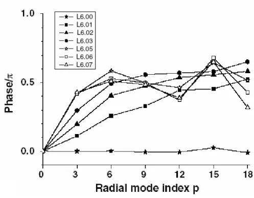
function of cavity tuning………5 Fig. 1-3 The relative phases of the LGp0 modes as L is tuned away from the

degeneracy………..6 Fig. 1-4 Calculated radial intensity distributions and the experimentally observed

beam profiles………..7 Fig. 1-5 The experiment data and the fitting line of the measured relaxation oscillation frequency at degeneracy and nondegeneracy……… 8 Fig. 1-6 The simulation data of the relaxation oscillation frequency via different

pumping power………...9 Fig. 2-1 The diagram of different threshold definitions………...17 Fig. 2-2 The log log scale diagram of steady-state photon number versus pumping rate with varying the coupling efficiency………18 Fig. 2-3 The log log scale diagram of steady-state photon number versus pumping rate with varying the spontaneous emission lifetime………..19 Fig. 2-4 The log log scale diagram of steady-state photon number versus pumping rate with varying the photon lifetime………..………20 Fig. 2-5 Frequency degeneracy in an optical cavity……….22 Fig. 2-6 The cavity length of common lower order degeneracy in the plano-concave

vii

Fig. 3-1 Experiment Setup………..……24 Fig. 3-2 The diagram of the reflective light of the He-Ne laser…………...………26 Fig. 3-3 The diagram of the transmissive light of the He-Ne laser…….….………26 Fig. 3-4 Transmitted power versus the focusing pumping……….………….27 Fig. 3-5 Experiment setup of pumping saturation method…….……….28 Fig. 4-1 The diagram of the pumping power versus the output power while using

R=8cm output O.C. at 1/4 degeneracy……….………30 Fig. 4-2 The log log scale diagram of experiment output power versus pumping

power………31 Fig. 4-3 The log-log scale diagram of steady-state photon number versus pumping

rate………32 Fig. 4-4 The log log scale diagram of the magnification part of Fig. 4-3………33 Fig. 4-5 Observed on-axis intensity versus cavity length for pumping power is 5 mW

at 1/4 degeneracy（L=4cm）by using small sot-size pumping………..35 Fig. 4-6 Observed off-cavity intensity versus cavity length for various gammas at 1/4

degeneracy（L=4cm）by using small sot-size pumping………35 Fig. 4-7 The lasing threshold versus different pumping spot size at 1/4 degeneracy

(L=6cm) and far away from 1/4 degeneracy (L=6.15cm)………37 Fig. 4-8. Observed on-axis intensity versus cavity length for various pumping power

by using large sot-size pumping………...37 Fig. 4-9 Observed off-cavity intensity versus cavity length for various pumping power by using large sot-size pumping………...38 Fig. 4-10 The output pattern ………39

1

Chapter 1 Introduction

Generally, the spontaneous emission rate were treated as an inherent process, namely, spontaneous emission of atoms would have been independent of the environment. However, the fact is that the spontaneous emission is not an immutable property of an atom but a consequence of atom–vacuum field coupling. It has long been recognized that the spontaneous emission of an atom in a resonator may be altered from the free-space value, because of a change in the density of modes [1]. In addition, it has not only been known that the rate of spontaneous emission is modified but also the pattern of spontaneous emission can be controlled [2]. The cavity-like effects are a classic theoretical problem which is called cavity quantum electrodynamics (cavity QED).

1.1 A brief review of cavity QED

There are two distinct regimes in cavity QED, i.e., the low-Q regime and the high-Q regime, where Q is the parameter of a resonator for the ability of conserving photon energy. The larger value of Q means that the resonator has smaller loss. A decisive parameter which separates these two regimes (low-Q and high-Q) is the vacuum Rabi frequency,

) 2 ( 0 0 12 12 V P P vac R _ε ω ε h h h = = Ω , _(1-1)

where P12 is the atomic dipole moment, εvac is the vacuum field amplitude and V0 is

2

the decay rate of the photon (γphoton）or the atomic dipole moment (γdipole), the

atom-vacuum field coupling is strongly perturbed by the cavity. In this situation, the spontaneous emission becomes reversible and coherent process. However, a laser system will not conform to this conduction because we need cavity loss to obtain sufficient laser output.

In the low-Q case, ΩR >> γphoton or γdipole, the cavity only weakly perturbs

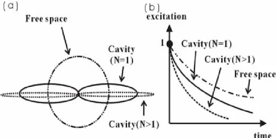
the atom-vacuum field. Spontaneous emission remains an irreversible and incoherent process. Nevertheless, the radiation pattern and the decay rate can still be modified by a cavity as show in Fig. 1-1. In Fig. 1-1 (a), the spontaneous emission will equally radiate to all directions in the free space; but it will be confined in a particular direction by a cavity. The enhancement of coupling strength is proportional to N , where N is number of atoms, which are collectively couple with the cavity field. So the pattern of spontaneous emission in Fig. 1-1 (a) is more localized for N > 1 with the faster decay rate in Fig. 1-1 (b) than for only one single atom in the cavity..

3

Fig. 1-1 Modified radiation pattern and decay rate of spontaneous emission intensity by free space, a cavity for a single atom (N=1), and a cavity for many atoms (N>1).

The sketch of Fig. 1-1 means that we could modify or control the pattern and the rate of spontaneous emission by a cavity or number of atoms. The modification of a spontaneous emission rate in the micro-wave cavity was first predicted by Purcell [1] in 1946, and Drexhage [3] demonstrated it by experiment in the late 1960s. After Purcell’s and Drexhage’s study, the study of cavity QED is toward optical cavity. The enhanced and inhibited spontaneous emission from atoms placed inside optical cavities had been observed by several groups [4]- [6].

Because of the interference in the micro-cavity, the amplitude of vacuum field is modified in the space. An atom where is located at node or anti-node of vacuum field will have different spontaneous emission rate, such as an atom at the anti-node will enhance spontaneous emission. We let atom as a harmonic oscillator which couples with vacuum field. The radiation intensity will be proportional to P12 εvvac

v _⋅

. Therefore the micro-cavity structures are suitable for controlling spontaneous

4

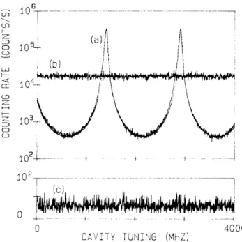
emission. Over the past decade, a considerable number of studies have been investigated cavity QED on micro-cavity semiconductor lasers [7][8]. Besides the micro-cavity, the cavity whose cavity length is much larger than the radiation wavelength can also observe the modification of spontaneous emission. In 1987, Heinzen et al., [9] studied on the decay rate of spontaneous emission in a macroscopic cavity which was operated with the confocal resonator. They found that the ytterbium atoms will have enhanced spontaneous emission rate when the atoms are resonant to the cavity mode, but inhibit far from the resonance. Curve (a) of Fig. 1-1 is the photon count rate while the cavity is open. The Airy function is measured by the spontaneous emission. It clearly shows that the spontaneous emission will be modified when the cavity is detuned. Curve (c) shows the counting rate with open cavity, but the laser detuned from the atomic resonance (background). In order to compare with curve (a) and to determine whether spontaneous emission is enhanced or inhibited, curve (b) is normalized counting rate with cavity blocked and multiplied by 2/(T1+T2) to compensate the interference in the cavity, where T1 and T2 are the transmittances of cavity mirrors. So curve (b) shows the counting rate in the free space. We can compare curve (a) and (b) to directly observe the enhanced and inhibited spontaneous emission.

5

Fig. 1-2 Photon counting rate for light transmitted through the cavity mirror, as a function of cavity tuning. (Ref. [9]). (a) counting rate with cavity open ; (b) in free space; and (c) background.

So far, the experiments about cavity QED can be categorized by two types. First, the micro cavity, e.g., in semiconductor, is used to modify vacuum field and then to control spontaneous emission. Another type of experiments, the mode density of macroscopic cavity is modified when the laser resonator operates at degenerate cavity configurations, e.g., mostly at the confocal or concentric cavity.

1.2 Motivation

In our previous study, there are many interesting phenomena occur in the tiny focused end-pumped Nd:YVO4 laser with degeneracy cavity. From the mode

decomposition [11], the transverse mode of degenerate cavity is consisted of the in-phase and frequency-locked degeneracy eigenmodes; which is referred to as the

6

so-called supermode. The results of mode decomposition were shown in Fig. 1-4. The degenerate eigenmodes have their relative phases except for those in the degenerate cavity. Furthermore, we used the character of supermode to directly generate the optical bottle beam at the degenerate cavity configurations [12]. A bottle beam has a low-intensity zone surrounded by a high intensity shell as shown in Fig. 1-4. The variation of transverse pattern along the propagation axis is caused by interference of the Gouy phases belongs to different degenerate transverse modes.

7

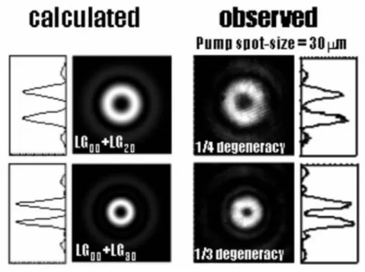
Fig. 1-4 Calculated radial intensity distributions and the experimentally observed beam profiles in Tai’s study. The calculated transverse profile of LG00 + LG20 is at z = zR and of LG00 + LG30 at z = zR/√3

that correspond to the photographs taken at 1/4 and 1/3 degeneracy, respectively.

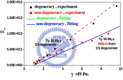
Recently, we observed that the relaxation oscillation at degeneracy is faster than that at nondegeneracy as shown in Fig. 1-5. We measured the relaxation oscillation frequency at the 1/3 degeneracy and 600µm away from the 1/3 degeneracy and calculated the life time of spontaneous emission by assuming the same photon lifetime for two cases. The relation between relaxation oscillation and spontaneous emission rate is given by

f cτ τ γ ω2 ₌ −1_, (1-2) where ω is the relaxation oscillation frequency, γ is the normalized parameter of pumping which is the pumping power divided by the threshold power, τc is the photon

8

time is determined by the cavity length and loss, with only 600µm cavity detuning (out of 2 cm to 8 cm), the photon life time should not change too much and it will be constant. So we use the Eq. 1-1 to fit the data of Fig. 1-5. The straight lines in Fig. 1-5 are the fitting results. The decay time of spontaneous emission at degeneracy is half of the value of 600µm away from the 1/3 degeneracy. We have the queer result that the spontaneous emission decay rate at degeneracy is less then the one at 600µm away from the 1/3 degeneracy.

0 2 4 6 8 10 0.00E+000 5.00E+011 1.00E+012 1.50E+012 2.00E+012 degeneracy , fitting non-degeneracy , fitting non-degeneracy , experiment degeneracy , experiment Tf: 33.83µs Tf: 55.99µs 1/3 degenerate 600µm from 1/3 degenerate

γ

ω

2 =P/ Pth

Fig. 1-5 The experiment data and the fitting line of the measured relaxation oscillation frequency at degeneracy and nondegeneracy.

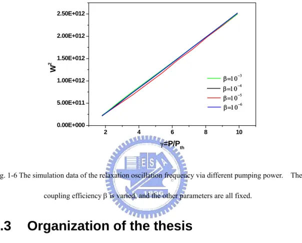
Then, we also consider the relation between relaxation oscillation frequency and the cavity. So we use the single mode rate equation with coupling efficiency β, which is given by eq. 2-1 and 2-2, to simulate the relaxation oscillation behavior by different β. Then, we can get the relaxation oscillation frequency by Fourier

9

transform. So, we can plot the relaxation oscillation frequency via different pumping power diagram is showed as follow. From this diagram, we can observe the coupling efficiency b does not affect the relaxation oscillation frequency so much.

2 4 6 8 10 0.00E+000 5.00E+011 1.00E+012 1.50E+012 2.00E+012 2.50E+012 W 2 γ=P/P_th β=10−4 β=10−5 β=10−6 β=10−3

Fig. 1-6 The simulation data of the relaxation oscillation frequency via different pumping power. The coupling efficiency β is varied, and the other parameters are all fixed.

1.3 Organization of the thesis

The first chapter describes the introduction and the brief review of cavity QED. The second chapter will present the theoretical backgrounds related to this study. Then the experiment setup and detailed experimental skills will be discussed in chapter three. In chapter four, we will discuss the result of the study. In the end, we conclude this thesis with prospective in chapter five.

10

Chapter 2 Theoretical background

2.1 The rate equation

In a single mode laser, we describe the upper level density N1 in the active

medium and photon number p in the cavity with the rate equations. The description of rate equations is valid as long as the dephasing time of dipole moment for the active medium is much short than the photon lifetime τc of cavity and the spontaneous

emission lifetime τf. It is must be noted that N1 will equal to population inversion in

an ideal four-level system.

A Nd:YVO4 laser is a four level system. Therefore the rate equations for the

Nd:YVO4 laser can be written as

p

V

g

N

V

dt

N

a f f a p

−

−

−

=

₁ 1

R

₍

1

_-

₎

d

τ

β

τ

β

(2-1) 1

)

-(

d

N

p

g

dt

p

f photon

_τ

β

γ

+

−

=

_. (2-2)

Here, RP is the pumping rate, β is the spontaneous emission coupling efficiency into

the lasing mode, and γphoton is the photon decay rate which is the reciprocal of τc (the

decay time constant in the passive resonator or photon lifetime). The second term on the right hand side of (2-1) indicates the spontaneous emission consisting of a fractional β of spontaneous emission coupling into the lasing mode and into the free space. And the spontaneous emission will contribute non-coherent photons to the cavity in the last term of (2-2). The gain operator g of active material is

11 approximately given by ) ( ' N₁ N₀ g g = − , (2-3)

where N0 is the certain upper -level density when the gain medium is transparency,

and g’ is the small signal gain which is proportional to the stimulate emission rate (A = 1/τf). The medium is transparent when its upper-level density is equal to the

lower-level density. In the ideal four-level laser system, the lower-level density is very small, but we still can estimate to be N0≒1013 under the Boltzmann distribution.

From the fundamental result of quantum theory, the spontaneous emission rate from any given set of atoms into any one individual cavity mode is exactly equal to the stimulated emission rate that would be produced from the same atoms by one photon of coherent signal energy present in the same mode. Therefore, we can write

f a V g'=

β

×

τ

(2-4) in Eq. 2-3.

2.2 Determining threshold

For an atom, there are two kinds of mechanisms to emit photon which are spontaneous and stimulated emission. It is must be noted that the stimulate emission needs an incident photon to bring out another coherent photon which is cloned from an excited atom. In the lasing process, most of photons are from stimulated emission, so that the laser photons possess the same polarization and direction. If we want to detect the spontaneous emission in a laser cavity, we must prevent from generating coherent photon. Therefore, it is essential to know how the threshold of laser is

12 defined.

The most widely used definition of the laser threshold is that the net stimulated emission gain should equal to the loss. Once pumping harder, the net stimulated emission will rapidly become the dominant emission source and lasing will take place. By inspecting (2-3) using the above-mentioned definition, the threshold can be expressed as ) (N ₁ N₀ V th f a photon − × = τ β γ . _(2-5)

So the population of upper level at threshold is

) 1 (1 V 0 0 1 _{β ξ} γ τ + = + = N N N a photon f th , (2-6)

where ξ is a dimensionless parameter defined by

photon f a V N γ τ β ξ ₌ 0 _. (2-7) Note that ξ can be interpreted as the photon number in the lasing mode when the gain medium is transparent (N1=N0). At this inversion level, there is no net stimulated

photon; and ξ is the ratio of spontaneous photon emitted into the lasing mode at transparency (

N

0

β

V

a

τ

f ) to the cavity loss (

γ

photon ). If this number is larger

than unity, substantial stimulated emission is occurred even at N1≦N0. In this case,

the threshold is determined by the material properties only. On the other hand, if ξ is much smaller than unity in (2-7), the threshold density of upper level is raised considerably. It means that the offset of cavity loss will change the threshold density, and the laser threshold is mainly determined by the cavity properties.

Before calculating the threshold power, the population inversion factor should be derived. When (2-5) is fulfilled, using the definition nsp≡N/(N-N0) and (2-6), the

13

ξ

+ = 1 1 ,th sp n . (2-8)

Substituting (2-6) and (2-8) into (2-1), the threshold pumping power can be given by ) (1 P ₁

ξ

β

νγ

+ = photon th h , (2-9)

where ν is the frequency of pumping source. If we decrease ξ by reducing the volume of the active medium, the threshold power will decrease accordingly until ξ << 1 when it is equal to

h

νγ

photon

β

. This threshold reduction is a classical

effect. In our laser, the lower level density is low, thus we can estimate ξ≒10-4 <<1. Therefore, the threshold power in our laser is given by

β

νγ

_photon th

h

=

1

P

_, (2-10)

and it depends mainly upon the properties of the cavity (β and γphoton). This means

the threshold power is dominated by a given cavity. One can reduce the threshold power by increasing the spontaneous emission coupling efficiency β without changing the volume of active medium at all, or by increasing β faster than the inverse of the volume of active medium. This effect is called the cavity QED effect. We believe that it can be a mixture of classical effect and cavity QED effect in our laser.

But the definition of the threshold described in (2-5) is unphysical, because the stimulated emission can never quite compensate for the optical loss. So Yamamoto brought up the other definition of threshold: the stimulated emission rate should be equal to the spontaneous emission rate at threshold other than the net gain should overcome the cavity loss. The rationale behind this definition is that half of the

14

photons emitted by the upper level atoms into the laser mode will be emitted coherently, and the other half of the photons will be added non-coherently, because there is equal probability for an upper level atom to emit a stimulated or a spontaneous photon. Upon pumping harder, both the coherent properties and the quantum efficiency will be improved quickly, in order to increase stimulated emission. From (2-3), we can get the relation of Nth, and it is given by

0

)

(

2

₂

−

₀

=

+

−

V

N

_th

N

f a photon

τ

β

γ

_{. (2-11)}

It can be further simplified as

)

1

2

(

2

2

0 0 2

_β

_ξ

τ

γ

+

=

+

=

N

V

N

N

a f photon th . (2-12)

Looking at (2-2), (2-3), and (2-4) at the steady-state, one easily finds that a new definition leads to a threshold photon number expressed as

2 , 0 2 2 2 N p _spth th th th n N N − = ≡ . _(2-13)

Here, Nth2 is the upper level density at threshold and nsp,th2 is the population inversion

parameter at this threshold. We substitute (2-11) and (2-13) into (2-1) and the threshold pumping power can be given by

) 1 )( 2 (1 2 P ₂

ξ

β

β

νγ

+ + = photon th h . (2-14)

In our laser, the lower level density is not large and ξ<<1 can be neglected. So the threshold power in our laser can be defined as

) 1 ( 2 P ₂

β

β

νγ

+ = photon th h . (2-15)

15

in the previous definition for very small β for the macro cavity.

A third threshold definition used is that the spontaneous emission rate shall equal the stimulated emission rate at threshold. The rationale behind this definition is that at this pump level, half of the photons emitted into the mode will be emitted coherently; the other half will be added noncoherently. On pumping harder, both the coherence properties and the quantum efficiency will improve rapidly due to the rapidly increasing stimulated emission. So, at this definition of the threshold, the mean photon number in the mode at threshold is unity:

1

P_th3 ≡ . _(2-16) Using this definition in (2-2) at steady state, we immediately get the upper level density at threshold,

)

1

1

(

2

2

)

(

0 0 3

_β

_ξ

τ

γ

+

=

+

=

N

V

N

N

a f photon th . (2-17)

The population inversion factor at this threshold can be given by

)

1

(

1

)

1

(

2

1

{

1

1

2 ,

₋

_>>

<<

+

≈

−

+

=

ξ

ξ

ξ

ξ

ξ

th sp

n

_. (2-18)

Here, the population inversion factor is -1, when ξ>>1. This is unphysical, and it means that this definition is not suitable when ξ>>1.

By substituting (2-17) and (2-18) into (2-1), we find that the threshold pumping power in use of the threshold definition in (2-16) will be

)] 1 ( 1 [ 2 P ₃

β

ξ

β

β

νγ

− + + = photon th h . (2-19)

Here, ξ<<1 for our laser system, the threshold power is roughly the same result as one for the second threshold definition (2-15).

16

2.3 The steady-state solutions

In steady-sate condition, where is dN1 dt=0 and dp dt =0, the photon number

and the upper level density will not vary with time. Then, we solve the upper level density and photon number at steady-state; and the solutions are given by

β β τ τ β τ β β τ τ β τ βτ τ τ β τ β τ ) 1 ( 2 ) ) 1 ( ) 1 ( ( 4 2 0 2 2 2 0 0 1 _{− +} + − + + − + + + + − − = a c f c p a c f c p f c p f a c a c V R V N R R V N V N N (2-20) f f c p a c f c p c p a cV R R N V R N p βτ τ β τ β β τ τ β τ β τ β β τ 2 ) ) 1 ( ) 1 ( 4 ) 1 ( ) 1 ( 2 0 2 2 0 − + + − + − + − + + − + = (2-21) or β β τ τ β τ β β τ τ β τ τ β τ β β τ ) 1 ( 2 ) ) 1 ( ) 1 ( ( 4 ) 1 ( ) 1 ( 2 0 2 2 0 1 _{− +} + − + + − + + + − + − = a c f c p a c f c p f c p a c V R V N R R V N N (2-22) f f c p a c f c p c p a cV R R N V R N p βτ τ β τ β β τ τ β τ β τ β β τ 2 ) ) 1 ( ) 1 ( 4 ) 1 ( ) 1 ( 2 0 2 2 0 − + + − + + + − + + − + = (2-23) There are two sets of solutions, but the second set of solution, that is (2-22) and (2-23),

is unphysical because the photon number is always negative. Therefore we will discuss the first set of solution and compare with my experimental results in the chapter four.

Use the parameters of our laser system which are listed as below in the calculation: τf ≈ 90 µs, N0 ≈ 1013 cm-3, Va=π×(10µm)2×(1mm) ,

17 ns mm cm s m cm l R R c l c [ ln(0.8 1) 2(5.5 10 )(1 )] 1 10 3 4 2 ] ' 2 ln [ 2 _{20 2 1} 2 8 1 2 1 _× − × + × ≈ × = + − = _α − − − τ , and 0.000012 2 ) 1 ( 4 (1064nm) 4 2 3 4 3 2 4 ≈ = ∆ = nm V n V_a λ π _a π λ

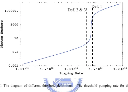
β . We can calculate these thresholds discussed above and show the three thresholds in the log-log scale diagram as follows.

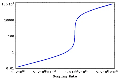
1.×1011 _1.×1012 _1.×1013 _1.×1014 _1.×1015 Pumping Rate 0.001 0.1 10 1000 100000. n o t o h Ps r e b m u N

Fig. 2-1 The diagram of different threshold definitions. The threshold pumping rate for the first definition is about 6.47817 x 1013_{; for the second definition is about 3.23915 x 10}13_{; for the third}

definition is about 3.23913 x 1013_.

Then, we vary the coupling efficiency β, and fix the other parameter. The diagram is showed as follow.

Def. 1 Def. 2 & 3

18 1.×1011 1.×1012 1.×1013 1.×1014 1.×1015 1.×1016 Pumping Rate 0.001 0.1 10 1000 100000. 1.×107 n o t o h Ps r e b m u N

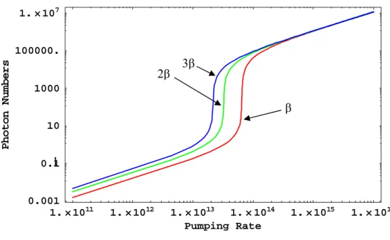
Fig. 2-2 The log log scale diagram of steady-state photon number versus pumping rate. The coupling efficiency is varied, and the other parameters are all fixed.

From Fig. 2-2, we conclude three phenomena: (1) Nothing would be gained by β when lasing; (2) The threshold will be modulated by β. The lower β is, the higher threshold is; and (3) The larger β is, the higher below-threshold population is.

Next, we fix the other parameters to see how the threshold varies with the spontaneous emission decay time τf in Fig. 2-3. In this diagram, the three curves are

completely overlapping to one another. Therefore, the spontaneous emission decay time τf does not affect the threshold behavior.

3β 2β

β

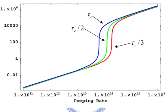
19 1.×1012 5.×101.12×1013 5.×101.13×1014 5.×101.14×1015 Pumping Rate 0.01 1 100 10000 1.×106 n o t o h Ps r e b m u N

Fig. 2-3 The log log scale diagram of steady-state photon number versus pumping rate. The spontaneous emission decay rate is varied and the other parameters are all fixed.

At last, let us see the influence of photon lifetime τc on the threshold. By

varying the photon lifetime τc to τc/2 and τc/3, although we knew the photon lifetime

τc can be expressed as 1 2 1 2 '] ln [ 2 _{− +} − = RR l c l c σ τ (2-24)

is basically not change with slightly changing cavity length l. Here R1,2 are the

reflectivity of the two mirrors, c is the speed of light, σ is the cross section, and l’ is the length of gain medium. In this equation, the photon lifetime τc can be varied by

changing the reflectivity of the output coupler R1 is listed as below.

The photon lifetime τc The reflection of the output coupler R1

τc/3 51%

τc/2 64%

20

We can observe two phenomena in Fig. 2.4: (1) The photon life time τc affects the

threshold as the well-known classical condition; and (2) The output photon number is not affected too much by the photon life time τc, whether the pumping rate (power) is

larger than the threshold or not.

1.×1011 1.×1012 1.×1013 1.×1014 1.×1015 1.×1016 Pumping Rate 0.01 1 100 10000 1.×106 t u p t u On o t o h Ps r e b m u N

Fig. 2-4 The log log scale diagram of steady-state photon number versus pumping rate. The photon life time is varied, and the other parameters are all fixed.

The discussion of the steady-state solutions in this section will compare with our experimental results later on in chapter four.

2.4 The position of degeneracy

We all know that the round trip phase shift (RTPS, 2θ =2kd) in the resonator with cavity length d, is almost but not quite an integral multiple of 2π radians.

3

/

c

τ

c

τ

2

/

c

τ

21

That deficiency is labeled by φ and is related to kd by

φ

π

θ

= 2 = 2 −

2 kd q , (2-25)

where q is now an integer. The phase shift experienced by a TEMn,m mode in

propagating from z=0 to z=d is given by

) ( tan ) 1 ( ) 0 ( ) ( 0 1 z d m n kd d −φ = − + + − φ , _(2-26)

so the resonance equation of typical two-mirror cavity is:

π 2 ) ( tan ) 1 ( 0 1 q z d m n kd− + + − = . _(2-27)

Then we can obtain a more easily interpreted formula [14] for the TEMn,m modes,

} 2 ) 1 ( { 2 . , ,

_π

ψ

ν

nm m n q q n m d c _{+ + +} = , (2-28)

where ψn.m is the Gouy phase angle, q is the longitudinal mode index, n and m are

the transverse mode indices. The Gouy phase angle is related to the cavity structure according to, 2 1 . 2 ₎ 2 1 ( cos ψ_nm =g g , (2-29) where g_1,2 =(1−d/R_1,2), with R the radii curvature of the two mirrors. Cavity _1,2

configurations such that the Gouy phase is a rational fraction of 2π , i.e., ) / ( 2 .m K N n π

ψ = , will lead to a ratio of transverse frequency spacing to longitudinal frequency spacing∆ν_T /∆ν_L =K /N. So we can present the typical frequency degeneracy in an optical cavity in a diagram as Fig. 2-5. The longitudinal mode spacing is

d c

2 , and the transverse mode spacing is cos ( ) 1 2 1 1 g g − π .

22

Fig. 2-5 Frequency degeneracy in an optical cavity.

According to the pervious discussion, we can also determine the cavity length of the frequency degeneracy in my laser system, which is a plano-concave structure with a 8 cm radius curvature output coupler in our experiment. The diagram of the cavity length of common lower order frequency degeneracy appears in Fig. 2-6.

Fig. 2-6 The cavity length of common lower order degeneracy in the plano-concave cavity with 8 cm curvature mirror.

23

Chapter 3 Experiment

In this chapter, we will discuss our experiment method and setup. Because we want to observe the variation of spontaneous emission in a laser system, we must operate laser below threshold. Inevitably we must deal with small signal of light; and the ratio of signal to noise (SNR) is very important in the measurement.

3.1 Experiment setup

The sketch of our experiment setup is shown in Fig. 3-1 (a) and (b). We use a tunable Ti: Sapphire laser as the pumping source which operates at continuous-wave (CW) with TEM00 mode and the output wavelength at 808 nm which is the absorption

peak of Nd: YVO4 crystal. The thickness of crystal is 1mm. The end face of the crystal which acts as the end mirror of the two-mirror cavity faced toward the pump beam had a dichroic coating with greater than 99.8% reflection at 1064 nm and greater than 99.5% transmission at the pump wavelength. The other facet is coated an anti-reflection layer at 1064nm to avoid the effects of intracavity etalon. The gain media is mounted on a translation stage to match the location of pumping beam waist. The output coupler（O.C.）with the radius of curvature is 8 cm has 20% transmission at the lasing wavelength 1064 nm, and mounted it on a motorize translation stage so we can scan the cavity length. In our experiment, we will concentrate on the degenerate cavity configurations. We use two light guides one of which sets behind the O.C. and the other sets at the side of cavity to collect the intensity of spontaneous

24

emission as shown in Fig. 3-1(a). Those two light guides connect to a Newport’s power meter which has sensitivity of sub-nW. To increase the SNR, we used a 1064 nm band pass filter to avoid measuring the pumping light of 808nm. In addition, we can observe the spontaneous emission pattern by a charge-coupled device (CCD) camera as shown in Fig. 3-1(b).

25

3.2 Aligning the laser system

In this section, we will introduce how do we setup our linear cavity of Nd： YVO4 laser. We will divide this section into three parts. At first, we will talk about

the rough alignment in the laser cavity. Then, we will clarify how to position the gain medium at the beam waist of pumping by using the pumping saturation effect. Finally, we will discuss the optimization of cavity alignment and acquaint with the process of measuring data.

3.2.1 Rough

alignment

To determine the optical axis is very important for a laser system. We use two equal-high apertures which are fixed on the optical table to set an optic axis. It must be noticed that the lasing (1064nm) and pumping (808nm) light are in infrared which is invisible. Invisible light is difficult to use for aligning the system. So we choose the He-Ne laser which is red light (632.8nm) to mark the optic axis. We let the He-Ne laser beam and the pump laser to simultaneously pass through two apertures to make sure those two beams overlap. Therefore, we can use He-Ne laser to align our optical components.

In this paragraph, we will discuss how to align optical components to the optic axis through checking the transmissive and reflective light of the He-Ne laser from the surfaces of optical components. As shown in Fig. 3-2 (b), if the reflection of the optical component is not return to the aperture, it means that the optical component is not perpendicular to optic axis. We should trim the angle of the optical component

26

to let the reflective light go back to the aperture like Fig. 3-2 (a). In addition, we must let the center of optical component to locate on the optic axis. Fig. 3-3 (b) shows that the center of optical component isn’t on the optic axis, in which the reflected light beam would not pass through the aperture. Then we should adjust the position of the optical component, in order to have the beam just pass through the aperture as Fig. 3-3 (a). Thus, this optical compoent is aligned.

Fig. 3-2 The diagram of the reflective light of the He-Ne laser.

Fig. 3-3 The diagram of the transmissive light of the He-Ne laser.

3.2.2 Determining pump waist at the crystal --- the

pumping saturation method

27

laser. Because the beam is focused so tightly, the Rayleigh range is very short. If we want to place the laser crystal at the beam waist of pumping, it will be very difficult by only estimating the distance between the pumping lens and the laser crystal. However, we can make use of the advantage of the pumping saturation effect to determine it.

Fig. 3-4 Transmitted power versus the focusing pumping.

To use a tightly-focused pump beam, it generally results very high pumping intensity which can easily exceed the pump-saturation intensity of material. When the pump beam is strongly focused in crystal, Fig. 3-4 indicates an increase of transmitted pump power which is discussed by G. Martel [16]. So we can record the residual transmitted pump power to identify the location of crystal. As shown in Fig. 3-5, the gain medium is fixed on a translation stage so that we can adjust the location of crystal quite accurately. The pump beam waist at the crystal is then determined by looking for the maximum transmitted pump power.

28

Fig. 3-5 Experiment setup of pumping saturation method.

3.2.3 Optimizing the laser system

Following above discussion, we should obtain some laser out although it may be very faint when raising the pump power. We need further fine alignment to optimize the laser system, the detailed alignment procedures are listed as follows:

1. Decrease the cavity length.

2. Fine tune the angle of the gain medium to make symmetric laser pattern. 3. Gradually increase the cavity length.

4. Fine tune the angle of the output coupler to make symmetric laser pattern. 5. Repeat the procedure1-4 several times until the output power and laser pattern would not change too much in the whole length of laser cavity tuning.

29

Chapter 4 Results & discussion

4.1 The enhancement of the spontaneous

emission

4.1.1 Determining the threshold

We all know that basically there are two kinds of emission processes that can occur in atoms or molecules. One is the spontaneous emission, and the other is the stimulated emission. There is always spontaneous radiation when the pumping power is less than the threshold and the stimulated emission starts to dominate the emission process when the pumping power is raised over the threshold. Here we are interested in measuring the spontaneous emission. It is essential to determine the lasing threshold in advance in order to ensure what we measure is the spontaneous emission while set the pumping below the threshold. In Fig. 4-1, by linearly fitting the linear plot of the output power versus the pump power, we can find the threshold at the 1/4-degeneracy is 20.22 mW.

However, we further use the second definition of threshold discussed in the chapter two and plot the output versus the pump power in log-log scale in Fig. 4-2 . In this figure, we observe different turning points for the 1/4-degeneracy and the non-degeneracy cavities. The turning point indicates that there is one coherent photon survived in the cavity. It clearly shows that the thresholds of 1/4-degeneracy

30

and non-degeneracy are different. The threshold at 1/4-degeneracy (L=4cm) is about 12mW, and the threshold at L=4.07cm and 3.93cm is about 45mW. Note that this threshold is about a half of 20 mW using the linear fitting (the first definition of threshold) as discussed in chapter 2. The equation of threshold can be written by

c th

cστ

1

P = , _(4-1)

where c is the speed of the light, σ is the stimulated emission cross section, and τc is

the photon life time.

20 25 30 35 40 45 50 0.0 0.5 1.0 1.5 2.0 2.5 3.0 3.5 4.0 4.5 5.0

Out

put power (m

W)

Pum ping pow er (m W )

y=-3.02941+0.14975x

Thershold =20.22m W

Fig. 4-1 The diagram of the pumping power versus the output power while using R=8cm output O.C. at 1/4 degeneracy.

From (2-24), we can immediately calculate τc= 1.195ns at 1/4-degeneracy,

τc=1.2ns at L=4.07cm, and τc=1.19ns at L=3.93cm, respectively. We found

indeed τc does not change too much when we only tune the cavity several

31

different cavity configurations? Why it always has the smaller threshold at the degeneracy than the non-degeneracy? Is it due to cavity QED effect?

10 100

Out

put Power

(a

.u.)

Pumping Power (mW)

L=3.93cm L=3.96cm L=4.07cm L=4.04cm L=4cm 45 13

Fig. 4-2 The log log scale diagram of experiment output power versus pumping power.

From Section 2.3, we know only the coupling efficiency β and the photon life time τc can affect the threshold. But the photon lifetime τc does not change too much

by tuning the cavity length. We therefore plot the diagram of output versus pump for τc= 1.195 ns, 1.2 ns, and 1.19 ns for the cavity at 1/4-degeneracy and L=4.07cm and

3.93 cm, respectively, in Fig. 4-3. It almost makes no change to the threshold. Even we magnify the portion around the threshold and show in Fig. 4-3 (b); the difference is too small to observe in our experiment. However, we do experimentally observe the minimal threshold occurring at degeneracy (L=4cm). The photon life time may affect the threshold but it is not the major cause in our

32

system to affect the threshold at the degeneracy and nondegeneracy.

1.×1011 1.×1012 1.×1013 1.×1014 1.×1015 1.×1016 Pumping Rate 0.001 0.1 10 1000 100000. 1.×107 n o t o h Ps r e b m u N Pumping Rate 10 50 100 500 1000 5000 10000 n o t o h Ps r e b m u N

Fig. 4-3 The log-log scale diagram of steady-state photon number versus pumping rate. (a) In real experiment, the change of photon life time is very small. So the phenomenon observation in experiment does not be affected by photon life time. (b) the magnification diagram of (a) around the

threshold. 13 10 5 . 5 × _7.5×1013 L=3.93cm (1.2ns) _{L=4cm (1.195ns)} L=4.07cm (1.19ns) (a) (b)

33

4.1.2 Different population at degeneracy and

non-degeneracy below the threshold

In Fig. 4.2, we not only found the lower threshold at the 1/4-degeneracy than at the nondegeneracy that may be due to the larger β but also found a slightly larger spontaneous emission at degeneracy for pumping below threshold in the magnified plot in Fig. 4-4. Compared with the discussion in the chapter two, we can conclude that the observed threshold phenomenon here is an evidence of larger coupling efficiency at degeneracy than at nondegeneracy.

8 9 10 11 12

Output Power (a.u.)

Pumping Power (mW)

L=4cm L=4.04cm L=4.07cm L=3.96cm L=3.93cm

Fig. 4-4 The log log scale diagram of the magnification part of Fig. 4-3. The different spontaneous emission output power between degeneracy and nondegeneracy with the same pumping power.

34

4.1.3 Spontaneous emission under small spot size

pumping

In this section we will describe the measured spontaneous emission intensity of the plano-concave Nd：YVO4 laser which is pumped by a small spot size about 10 µm.

The spontaneous emission measured on the optic axis show being enhanced in Fig. 4-5 at the degeneracy cavities, i.e. 1/5, 1/4, 1/3, 2/5 degeneracy…, etc. The dash line indicates that the collection efficiency of the spontaneous radiation as a function of distance between the light guide and the gain medium while tuning the cavity length from 2 cm to 12 cm. At the edge of the stable region (L=8 cm), there are many degeneracy, e.g., 3/7, 2/9, 5/11 and 1/2, which are squeezed all together. The phenomenon at the edge of the stable region is too complicated to examine in detail here. Therefore, we will focus our attention on the modulation of the spontaneous emission around 1/4 degeneracy cavity (L=4 cm).

The measured emission intensity off the cavity to the free space versus the cavity length is shown in Fig. 4-6. The off-cavity spontaneous emission shows inhibited at the degeneracy even when the pumping power is lower than the threshold. The results are contrary to our ordinary recognition of spontaneous emission that is not influenced by the macro-cavity. Based on the observations in Fig. 4-5 and Fig. 4-6, we bring up Heinzen’s idea that the spontaneous emission is coupled into the cavity mode is actually observable at degeneracy. However, one may wonder in what conditions the phenomenon of modulating spontaneous emission can be observed? This will be discussed in the next section.

35 2 4 6 8 10 12

Power

(

a.u.)

Cavity length (cm)

1/5 1/4 1/3 2/5

Fig. 4-5 Observed on-axis intensity versus cavity length for pumping power is 5 mW at 1/4 degeneracy （L=4cm）by using small sot-size pumping.

3.7 3.8 3.9 4.0 4.1 4.2

Powe

r (a

.u.)

Cavity length (cm)

0.2 0.4 0.6 0.8 1 1.4 1.8 2.2 2.6 3 Gamma

Fig. 4-6 Observed off-cavity intensity versus cavity length for various gammas at 1/4 degeneracy （L=4cm）by using small sot-size pumping.

36

4.1.4 Spontaneous emission under large spot size

pumping

In our previous study, we knew that the lasing threshold at 1/4 degeneracy (L= 6 cm) is different from the cavity slightly tuned away from 1/4 degeneracy at L = 6.15 cm for O.C. having radius of curvature of 8 cm and 10% transmission, when the pumping spot size is less than 80μm as indicated in Fig. 4-7. In this section we will repeat the experiment of Section 4.1.3 but change the pumping lens to increase the pumping spot size to 80 µm. The results appear in Fig. 4-8. We found the on-axis spontaneous emission is clearly not modulated by the cavity. The measured results follow decaying trend as the dash curve in Fig. 4.5 that caused by the farther distance of the light guide from the gain medium. In Fig. 4-9, the intensity of off-cavity spontaneous emission is also not modulated by the cavity even when the pumping is set below the threshold. But the spontaneous emission is still affected by cavity when the pumping is higher than the threshold at 180 mW pumping. At degeneracy, the lasing mode will have good overlap with pumping. It takes most the stored energy from the inversion population, so that a spontaneous emission dip is observed at degeneracy when the laser is pumped above the threshold..

37

Fig. 4-7 The lasing threshold versus different pumping spot size at 1/4 degeneracy (L=6cm) and far away from 1/4 degeneracy (L=6.15cm).

2 4 6 8 10

Power

(a.u.)

Cavity length (cm)

5mW 20mW 50mW 50mW 20mW 5mW

Fig. 4-8. Observed on-axis intensity versus cavity length for various pumping power by using large sot-size pumping. 20 40 60 80 100 120 0 5 10 15 20 25 30 35 40 L = 6.15 cm L = 6 cm

La

s

ing t

h

re

s

hol

d (

m

W

)

Pump size (

µ

m)

38 0.03 0.04 0.05 0.06 0.07 0.08 0.09 0.10 0.11 10mW 30mW 50mW 1/2 1/3

Power (a.

u

.)

Cavity length (m)

180mW 50mW 30mW 10mW 1/4 180mW

Fig. 4-9 Observed off-cavity intensity versus cavity length for various pumping power by using large sot-size pumping.

4.2 Modified pattern of spontaneous emission

In this section, we will use a CCD in the experimental setup (Fig. 3-1(b)) to monitor the emission pattern. The photograph in Fig. 4-10(a) is the far-field pattern of spontaneous emission taken at the 1/4-degeneracy at the pump power equals to 12mW which is just below the threshold. We also observed similar pattern of spontaneous emission at 1/3 degeneracy for 10 mW pumping in Fig. 4-10(b). However, there are no specific emission structured patterns other than uniform ones for the nondegenerate cases that may be only 1.5 mm away from the degeneracy. This is a concrete evidence of coupling the spontaneous emission to the lasing mode

39

at the degeneracy that causes modifying the pattern of dipole radiation of Nd3+ ions in YVO4 matrix.

Fig. 4-10 The output pattern (a) from a laser pumped by 12 mW at the 1/4 degenerate cavity; (b) pumped by 10mW at 1/3 degeneracy.

40

Chapter 5 Conclusion and feature works

5.1 Conclusion

In conclusion, the anomalous spontaneous emission has been observed in the degeneracy resonator under tiny-focused pumping. Direct measurement of the relaxation oscillation frequency reveals that the spontaneous emission rate can be affected by the degeneracy resonator structure. For the macro-cavity like our laser system, the laser threshold using the second definition should mainly be determined by the coupling efficiency of spontaneous emission to the laser cavity and the photon lifetime. Due to only slightly tuning the cavity length in the whole experiment performed in this study, there is very limit change of photon lifetime, in turn, the photon lifetime has very limit influence on the observed anomalous spontaneous emission. We observed the larger coupling efficiency β accompanied with the lower threshold at degeneracy as compared with those at nondegeneracy. Furthermore, the spontaneous emission has been strongly modified by the cavity with directionality even with the pump power is set far below the lasing threshold. Nevertheless, the enhancement spontaneous emission at degeneracy is not observable with large pump size in which the laser shows the same thresholds for both degenerate and nondegenerate cavities. Therefore, the mode volume or ξ may be essential for discussing the anomalous spontaneous emission at degenerate for macro-cavity lasers even though ξ is much less than 1 in the macro cavity.

41

5.2 Future works

In our previous studies, we had revealed that there are many interesting phenomena in the degeneracy laser cavity under tiny-focused pumping, for example, frequency mode-locking, optical bottle beam, and anomalous spontaneous emission behavior, which is discussed in this thesis. Therefore, in the future work, we will continue to investigate on the anomalous spontaneous emission and to find out whether the spontaneous emission is really enhanced by directly measuring the spontaneous emission lifetime and enhancement ratio. Furthermore, we shall make sure this effect can reduce the noise and improve the modulation speed. As mentioned above, there is a boundary of pump size that would separate the anomalous spontaneous emission behavior with the normal one. Is it also the boundary for the quantum and the classical laser systems?

42

References

1. E. M. Purcell, Phys. Rev. 69, 681（1946）.

2. Y. Yamamoto, S. Machida, Y. Horikoshi, K. Igeta, Opt. Commun. 80, 337 （1991）.

3. K. H. Drexhage, Progress in Optics, 12, 163 (1974)

4. P. Goy, J. M. Raimond, M. Gross, and S. Haroche, Phys. Rev. Lett. 50, 1903 （1983）.

5. R. G. Hulet, E. S. Hilfer, and D Kleppner, Phys. Rev. Lett. 55, 2137（1985）. 6. F. De Martini, G. Innocenti, G. R. Jacobovitz, and P. Mataloni, Phys. Rev. Lett.

55, 2955（1987）.

7. Yoshihisa Yamamoto, Susumu Machida, and G. Björk, Opt. and Quant. Electr. 24, S215（1992）.

8. Y. Yamamoto, F. Tassone, H. Cao. Semiconductor Cavity Quantum Electrodynamics （Springer, 2000）.

9. D. J. Heinzen, J. J. Child, J. E. Thomas, and M. S. Feld, Phys. Rev. Lett. 58, 1320（1987）.

10. D. J. Heinzen, and M. S. Feld, Phys. Rev. Lett. 59, 2623, （1987）.

11. Ching-Hsu Chen, Po-Tse Tai, and Wen-Feng Hsieh, Opt. Commun. 241, 145 （2004）.

12. Po-Tse Tai and Wen-Feng Hsieh, and Wen-Feng Hsieh, Opt. Express, 12, 5827, （2004）.

13. Paul R. Berman, ed. Cavity Quantum Electrodynamics. P. 232 (Academic Press, 1994).

43

14. A. E. Seigman , Laser ( Mill Valley ,CA ,1986 )

15. W. Koechner, Solid-State Laser Engineer, 4th, P.84, Eq. (3.15) （Springer, 1995） 16. G. Martel, C. Ozkul, and F. Sanchez, Opt. Commun., 185, 419 （2000）.