基於影像特徵點擷取結合深度資訊之即時手勢辨識系統設計

(1)

國立交通大學

電控工程研究所

碩士論文

基於影像特徵點擷取結合深度資訊之

即時手勢辨識系統設計

Real-Time Hand Gesture Recognition System

Design Based on Image Feature Points Extraction

and Depth Information

研究生：吳仕政

指導教授：陳永平教授

(2)

基於影像特徵點擷取結合深度資訊之

即時手勢辨識系統設計

Real-Time Hand Gesture Recognition System

Design Based on Image Feature Points Extraction

and Depth Information

研究生：吳仕政 Student：Shi-Cheng Wu

指導教授：陳永平 Advisor：Professor Yon-Ping Chen

國立交通大學

電控工程研究所

碩士論文

A Dissertation

Submitted to Institute of Electrical Control Engineering College of Electrical and Computer Engineering

National Chaio Tung University In Partial Fulfillment of the Requirements

For the Degree of Master In

Electrical Control Engineering June 2013

Hsinchu, Taiwan, Republic of China

中華民國一百零二年六月

(3)

i

基於影像特徵點擷取結合深度資訊之

即時手勢辨識系統設計

學生: 吳仕政指導教授: 陳永平教授

國立交通大學電控工程研究所

摘要

近年來，手勢辨識可應用的領域相當廣泛，因此受到重視且被深入的研究與探討，例如人機溝通、遠距遙控等皆是。一般而言，手勢辨識系統先根據手勢模型找出其特徵，再利用這些特徵來做辨識。本篇論文提出以 Kinect 之彩色及深度影像為基礎的手勢特徵擷取，來設計即時手勢辨識系統。整個系統分成三個部分：前景偵測、特徵擷取及手勢識別。首先利用膚色偵測配合聯通物件法濾掉背景並找出可能的手勢範圍；之後藉由距離轉換並尋找距離轉換區域的最大值來萃取特徵點，進而利用特徵點找出手勢特徵，包括手的方向、掌心位置、指尖位置及指向。最後，設計以手勢特徵為依據之即時手勢辨識系統，從實驗結果可知，本論文所提之手勢辨識系統確實可以達成具有成效之即時辨識功能。

(4)

ii

Real-Time Hand Gesture Recognition System

Design Based on Image Feature Points

Extraction and Depth Information

Student：Shi-Cheng Wu Advisor：Prof. Yon-Ping Chen

Institute of Electrical Control Engineering

National Chiao-Tung University

ABSTRACT

In recent years, hand gestures recognition(HGR) approaches have been widely applied to a diversity of areas, like human-computer interface(HCI) and remote control systems. The HGR systems usually rely on a hand model to extract useful hand gesture features. This thesis proposes a robust and fast feature extraction method for hand gesture based on the depth and RGB information from Kinect to implement a real-time HGR system. The system is divided into three parts, including region-of-interest (ROI) selection, feature extraction and hand gesture recognition. First, the skin color detection and connected component labeling(CCL) are applied to

select the potential ROIs. Then, pixels with local maximum

distance-transformation-value in the potential ROIs can be extracted as feature points. Further, these feature points could be used to find hand gesture features such as hand orientation, palm center and fingertip positions and directions. Finally, the extracted hand gesture features are send into the HGR system. From the experimental results, the proposed hand gesture recognition system can perform in real-time and possess good recognition rates.

(5)

iii

Index of Tables

Table 1.1 Specification of Kinect ... 3

(10)

viii

(11)

1

Chapter 1 Introduction

1.1 Preliminary

In recent years, the hand gesture recognition(HGR) becomes a popular subject since it provides a natural and intuitive communication for human-computer interaction(HCI). There are many applications using HGR such as video games and robot control. However, HGR is a complex issue because our hands consist of many connected joints and high order degree of freedoms(DOFs). To reach a real-time HCI via hand gestures, it has to meet some requirements such as computation time, accuracy and robustness against different background. Earlier HGR researches used data gloves or makers to make image processing easier and more accurate [15], but they are not convenient for users and thus recent investigators pay more attentions to recognizing bare hand gestures without the aid of any gloves or makers.

The HGR techniques can be classified into three categories: color-based algorithms, appearance-based algorithms, and 3-D hand model-based approaches. Color-based algorithms directly apply the image color to model the visual appearance of the hand by searching the skin colored regions in the image [1]. Although it has a good real-time performance, it's very sensitive to lighting condition and often results in false detection of other skin-like objects. As to the appearance-based algorithms, they compare these parameters of the selected features related to visual appearance or mathematical transformation of hands [4-11]. Most of the appearance-based methods are pixel based, so the computation cost is usually too high to implement in real time systems. For the 3-D hand model-based approaches, they depend on the 3-D

(12)

2

kinematic hand model with a large scale of DOFs and estimate the hand parameters by comparing the difference between input images and possible 2-D appearance projected by a 3-D hand model [3,16]. This model generally provides a rich information to recognize a wide class of hand gestures, but a huge image database is required to cover all the possible shapes under different views. Meanwhile, matching every input frame image with the whole image database will lead to a large amount of time consumption in computation. In this thesis, a color-based algorithms is used to select the image ROI.

In general, the system could be separated into three stages: foreground segmentation, feature extraction, and hand gestures recognition. Foreground segmentation is implemented to select the region of interest(ROI) and filter out the background region. Therefore, the remaining search region would be reduced such that the processing speed could be highly enhanced. Furthermore, the appropriate features would be extracted to distinguish different gestures efficiency and correctly. Finally, the selected features would be used as the input of hand gestures recognition system to get the final result. The related methods would be introduced in the following sections.

(13)

3

1.2 System Overview

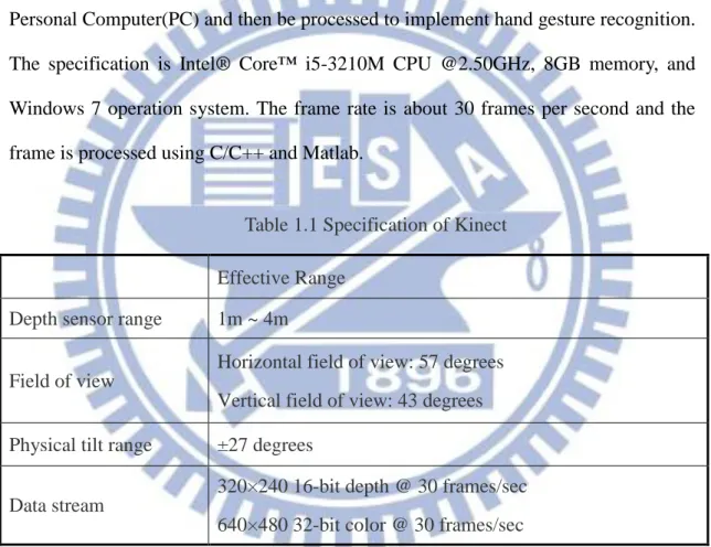
For the hardware architecture, our system uses Xbox Kinect as the image sensor, including RGB image and depth information, and Table 1.1shows the specification of Kinect. In the depth image, the pixel with lower intensity indicates that the distance between object and camera is smaller, and all the points are set to 0 if the sensor is not able to measure their depth. The image captured by Kinect would be delivered into Personal Computer(PC) and then be processed to implement hand gesture recognition. The specification is Intel® Core™ i5-3210M CPU @2.50GHz, 8GB memory, and Windows 7 operation system. The frame rate is about 30 frames per second and the frame is processed using C/C++ and Matlab.

Table 1.1 Specification of Kinect Effective Range

Depth sensor range 1m ~ 4m

Field of view

Horizontal field of view: 57 degrees Vertical field of view: 43 degrees Physical tilt range ±27 degrees

Data stream

320×240 16-bit depth @ 30 frames/sec 640×480 32-bit color @ 30 frames/sec

For the software architecture, Fig- 1.1 is the flowchart of the proposed system. At first, the system receives the RGB and depth images from Kinect and then selects the region-of-interest (ROI). After ROI selection, the feature extraction is implemented. At the final stage, the overall features are delivered into the hand gesture recognition system to distinguish different gestures. The experimental environment is our laboratory and the Kinect camera is at about 100cm height.

(14)

4

Moreover, there are two limitations when implementing the system: first, the detection distance is between 0.5m to 2m because of the hardware limitation of Kinect. Second, the system only focus on one-user implementation.

Chapter 2 describes the related works of the system. Chapter 3 introduces the proposed system in detail. Chapter 4 shows the experimental results. Chapter 5 is the conclusions of the thesis and the future works.

(15)

5

Chapter 2 Related Works

2.1 Hand Gesture Recognition Method

In recent years, many hand gestures recognition approaches have been proposed. In general, the overall methods could be roughly divided into three categories: color-based algorithms, appearance-based algorithms, and 3-D hand model-based approaches. 3-D hand model-based approach [3,16] relies on the 3-D kinematic hand model with a large scale of DOF and calculates the hand parameters by comparing the difference between the input images and the possible 2-D appearance projected by the 3-D hand model. This approach is suitable for the realistic interactions in virtual environments since it provides a rich information to describe different type of gestures. However, the major drawback is that requires a huge image database to deal with the entire characteristic shapes under different views.

The skin color are the image features that are frequently used for hand detection[1]. However, color-based algorithms face the difficult task that human arm and face have the similar color with hands. This methods also very sensitive to the lighting conditions. So when the lighting does not satisfy some environment requirements, this algorithm usually perform not well.

For the appearance-based algorithms, shape descriptors are used to represent the hand shape. In [4] , Fourier descriptor and Zernike moments are used to recognize hand gesture, but the computational cost is too high since it's pixel based algorithm. [5] obtained the integrated hand contour and then computed the curvature of each point

(16)

6

on the contour, but the noise and the unstable illumination in the segmented background are the major problems for this method. The eigenspace is another technique, which provides an efficient representation using a set of basis vectors, but this method is not invariant to translation, scaling, and rotation. For the reason, a number of researchs on local invariant features, such as SIFT and Haar-like features, are proposed. In [6], SIFT features are used to achieve rotation invariant hand detection. The authors of [7] used Haar-like features, which describe the ratio between dark and bright regions rather than single pixel value, to reach a hand gestures recognition, but the computation cost makes it hard to implement on real-time systems.

Another appearance-based approaches focus on building a hand model containing the palm and finger structures. [8] determined the fingertip positions and the center of the palm using the first moment of the 2-D probability distribution that based on the contour of the hand segmented region. [9] detected the fingertips using the momentum of the skin color region and used the Kalman filter to reach a robust finger tracking. Since there are a number of pixels on the contour or edges, so the computation cost for both [8] and [9] are considerably high. Template matching can also be used to detect fingertips and palms [10] , but the distance from camera to hand cannot be changed and a good hand segmentation results are also required. [11] proposed a method that combines particle filtering with particles random diffusion. However, the cost of this method is still too high to implement.

(17)

7

2.2 Skin Color Segmentation

This is an important step to extract all skin pixels from the Kinect sensor. Most skin color segmentation methods are based on the statistical approach, which can be divided into two categories: parametric and non-parametric. The parametric statistical approach, such as Gaussian model, Gaussian-mixture model, etc., represents the probability density function(PDF) of skin-color distribution in a parametric form. The main advantages of this approach are lesser computation time and no training data to be saved. However, a suitable parametric order, especially for Gaussian-Mixture model case, is hard to determined and may not fit the real skin-color distribution. Non-parametric approach uses quantized histogram to represent the PDF, or uses training data to estimate the skin-color density function, such as the kernel method or support vector machine(SVM). Although this approach can be evaluated intuitively and adequate to different training data sets, a major drawback is that it requires to keep a larger amount training data and costs a relatively high computation time. Consequently, model selection is a trade-off between proper fitting and computation complexity.

The choice of color space is considered as the primary step in skin-color segmentation. The statistical approaches usually use a suitable color space to reduce the effect of varying luminance and decrease the overlap between skin and non-skin pixels. Usually, HSV and YCbCr are most popular color space for skin detection due to the robustness of varying illuminant and the minimum overlap between skin-color and background-color [12] .

The parameters of the GMM can be obtained from the training data through the iterative expectation-maximization (EM) technique [13] . After proper parameter

(18)

8

estimation, both conditional probability densities for skin and non-skin colors are obtained, denoted as p(X | skin) and p(X | nonskin), where X = [Cr Cb]T. Given this class conditional probabilities of skin and non-skin models, a skin classifier can be built using Bayes classifier [14] . The classification boundary is determined where the likelihood ratio of p(X | skin) and p(X | nonskin) exceeds some threshold based on the ROC(receiver operating characteristics) curve. That is, for a given image pixel xn =[Cr(n) Cb(n)]T, it is classified as skin when it satisfies:











 



| | | | n n n n

p skin p skin p skin

K p nonskin  p nonskin p nonskin 

x x

x x (2.1)

where K is a constant and p(skin)  1p(nonskin). Rearranging (2.1), it becomes:













| ' | 1 n n p skin p nonskin K K p nonskin  p nonskin x x (2.2)

The threshold K' is usually determined from the ROC curve, which shows the relationship between the true positives and false positives. The Bayes classifier has been widely used for skin segmentation since its simplicity and less computation time. We only need to compute the likelihood ratio in (2.2) and check whether it is larger than the threshold K'.

(19)

9

2.3 Classification From Linear Model to ANNs

The goal of classification problem is to assign an input data xn X, n = 1,2,...,N,

in the database, to one of the K classesC_k, k = 1,2,..,K. Usually, these classes are disjoint such that xn is classified into at most one (or none of them). To simplify the

discussion in this section, here we only consider the model for two-class classification problems.

2.3.1 Linear Model

To determine which class an input xn belongs to, the simplest decision function

for two-class classification problems is usually given as the following linear model:

0 0

T

n j nj

j

yw x w 



w x w (2.3)

where w is called the weighting vector and w0 is the bias. Based on the linear model

(1), first choose y=0 as the decision boundary, and then classify the inputs satisfying y ≧0 into the class 1, denoted as C1, and the other inputs into C2. An example for the

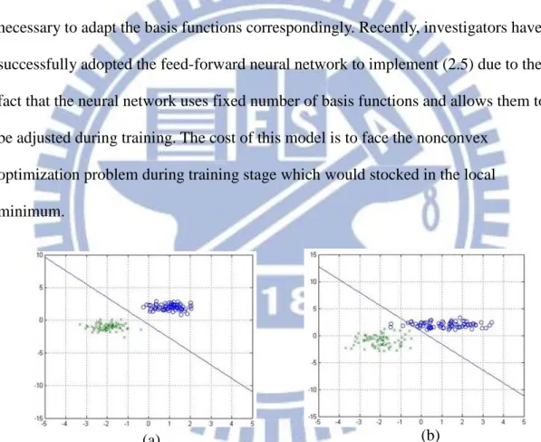
above two-class classification is shown in Fig- 2.1 (a), where the decision boundary is included. However, this linear model does not work well when there exists an overlap between the two classes, such as the XOR problem depicted in Fig- 2.1 (b). To solve this problem, a generalized linear model is proposed.

2.3.2 Generalized Linear Model

The idea of generalized linear model is to transform the input data xn in the

database X into another space, and then uses the transformed data as a substitute of xn

in (2.3), described as below:

 

0

T n

(20)

10

where φ(‧) is a user defined basis function. In other words, the basis function transforms the databaseX to the linearly separable feature space. Moreover, an activation function f(‧) can be further introduced to modify (2.4) as below:

 



0



(

 

0) T n j j n j y f w φ x w  f



w x w (2.5)

which y represents the predicted discrete class labels, or posterior probability lying in the range [0,1]. However, an adequate basis function φ(‧) is often difficult to

determine. In order to apply the modified model (2.5) to a variety of problems, it is necessary to adapt the basis functions correspondingly. Recently, investigators have successfully adopted the feed-forward neural network to implement (2.5) due to the fact that the neural network uses fixed number of basis functions and allows them to be adjusted during training. The cost of this model is to face the nonconvex

optimization problem during training stage which would stocked in the local minimum.

2.3.3 Artificial Neural Network

ANNs have been successfully applied to some complicated problems, such as image analysis, speech recognition, adaptive control, etc. Usually, the ANNs will be adopted to implement human detection via intelligent learning algorithms. The basic

Fig- 2.1 The examples for (a) linear separable set (b) linear inseparable set

(21)

11

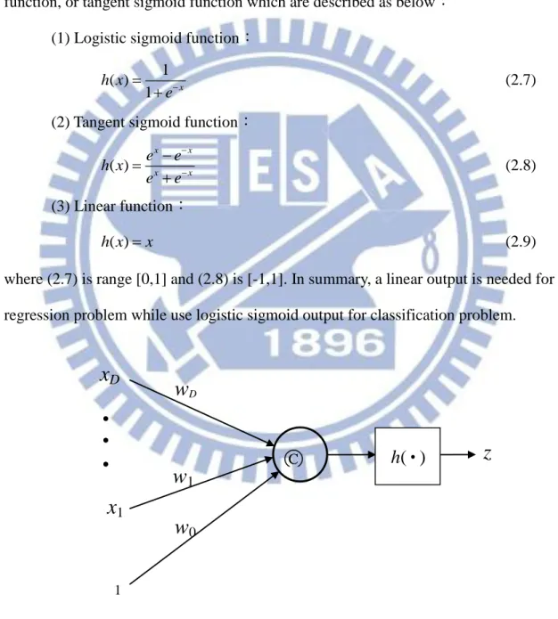
structure of ANNs is called neuron, whose input-output relationship is shown in Fig- 2.2 and described as 0 0 1 ( ) ( ) D T i i i z h w h w x w   w x 



 (2.6)

which has the same form as (1) with the output z and the input x =[x1,x2,...,xD]T  D

.

Usually, the activation function h(‧) is chosen to be logistic sigmoid function ,linear function, or tangent sigmoid function which are described as below：

(1) Logistic sigmoid function： 1 ( ) 1 x h x e   (2.7)

(2) Tangent sigmoid function： ( ) x x x x e e h x e e      (2.8) (3) Linear function： ( ) h x x (2.9)

where (2.7) is range [0,1] and (2.8) is [-1,1]. In summary, a linear output is needed for regression problem while use logistic sigmoid output for classification problem.

x

1

z





Fig- 2.2 Basic structure of a neuron

h(‧)

w

1

w

D

x

D 1

w

0

(22)

12

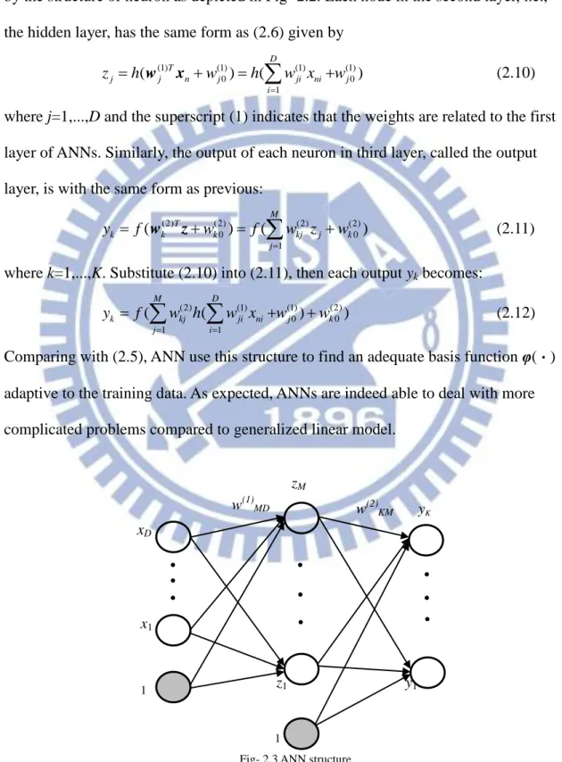
A general ANN is composed of one input layer, one output layer, and one hidden layer, as shown in Fig- 2.3. The input layer just receives input signals, so each node in this layer is taken as a buffer. For the other two layers, their nodes are realized by the structure of neuron as depicted in Fig- 2.2. Each node in the second layer, i.e., the hidden layer, has the same form as (2.6) given by

(1) (1) (1) (1) 0 0 1 ( ) ( ) D T j j n j ji ni j i z h w h w x w   w x  



 (2.10)

where j=1,...,D and the superscript (1) indicates that the weights are related to the first layer of ANNs. Similarly, the output of each neuron in third layer, called the output layer, is with the same form as previous:

(2) (2) (2) (2) 0 0 1 ( ) ( ) M T k k k kj j k j y f w f w z w   w z 



 (2.11)

where k=1,...,K. Substitute (2.10) into (2.11), then each output yk becomes:

(2) (1) (1) (2) 0 0 1 1 ( ( ) ) M D k kj ji ni j k j i y f w h w x w w   



  (2.12)

Comparing with (2.5), ANN use this structure to find an adequate basis function φ(‧) adaptive to the training data. As expected, ANNs are indeed able to deal with more complicated problems compared to generalized linear model.

1 w(1)MD wj0 xD x1 1 z1 y1 yK kK w(2)KM zM

(23)

13

2.4 Classification for Sequential Data

The learning algorithms mentioned before such as linear model and ANN are primarily focused on the independent and identically distributed(i.i.d.) observations. The i.i.d. assumption allows us to express the likelihood function of all observations as:



1 2 N





1

 

2





N



p x x, ,...,x |  p x | p x | p x | (2.13) where xn is the observation at time n, n1,...,N, and  is a user-defined parameter.

However, this assumption would fail in many applications when the observations are sequential and depend on the previous ones, like speech data, rainfall measurements, etc.. Therefore, it is necessary to consider the correlation among all observations. But in real application, it would be difficult to find a general dependence of present observation to all previous observations since the complexity would grow as time increases. To solve this problem, Markov model is proposed under the assumption that the present data xn only depends on the previous one xn-1.

2.4.1 Markov Model

Given N observations {x1,..., xN }, we can always use the product rule to express

the joint distribution for this sequence of observations as below:





  

 







 





1 1 2 1 3 1 2 1 1 1 1 1 2 ,..., , ,..., ,..., x x x x | x x | x x x | x x x x | x x N N N N n n n p p p p p p p     



(2.14)

where Fig- 2.4 shows the fully dependent sequence, that is, the observation xn at time nis correlated to all the previous n1 observations. Assume that each of the

(24)

14 distribution in (2.14) can be simplified as:



n| 1,..., n 1





n| n 1



, 1, 2,...,

p x x x   p x x  n N (2.15)

Therefore, the joint distribution of N observations is rewritten as



1



 

1



1



2 ,..., | N N n n n p p p _  



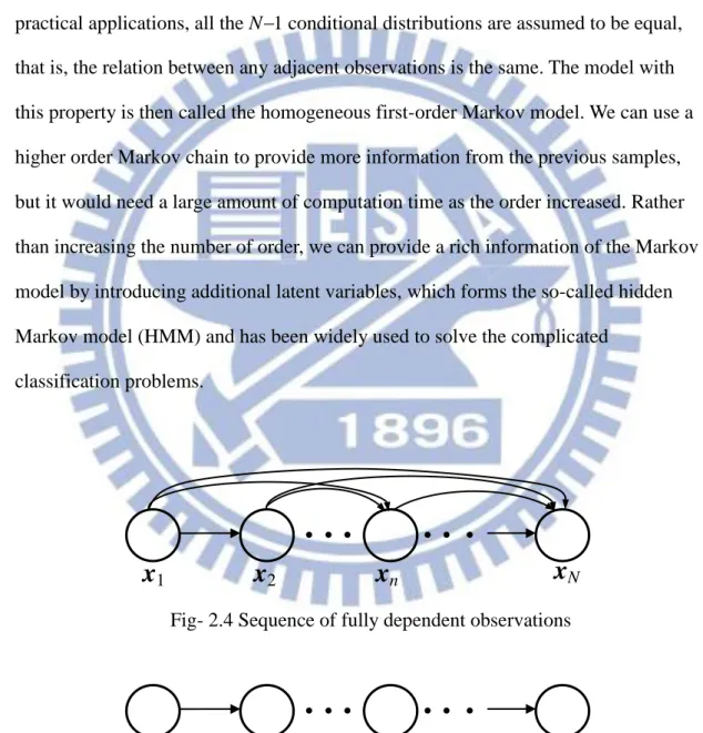
x x x x x (2.16)

which is known as the first-order Markov chain and shown in Fig- 2.5. In most practical applications, all the N1 conditional distributions are assumed to be equal, that is, the relation between any adjacent observations is the same. The model with this property is then called the homogeneous first-order Markov model. We can use a higher order Markov chain to provide more information from the previous samples, but it would need a large amount of computation time as the order increased. Rather than increasing the number of order, we can provide a rich information of the Markov model by introducing additional latent variables, which forms the so-called hidden Markov model (HMM) and has been widely used to solve the complicated

classification problems.

x1

Fig- 2.5 Sequence of first-order Markov chain

x2

x

_n

x

N

x

1

Fig- 2.4 Sequence of fully dependent observations

(25)

15

2.4.2 Hidden Markov Model

The HMM depicted in Fig- 2.6 includes 1st-order Markov chain Z{z1 ,..., zN}

where zn is the latent variable, or called hidden state, corresponding to the observation

data xn, n1,...,N. It is obvious that zn is only related to the previous latent variable zn-1

and the resulted joint distribution is given by:



x , ..., x , z , ..., z1 N 1 N



  

z1 x | z1 1

 

z | z2 1





z | zN N 1

 

x | zN N



p  p p p p _ p

 

1



1







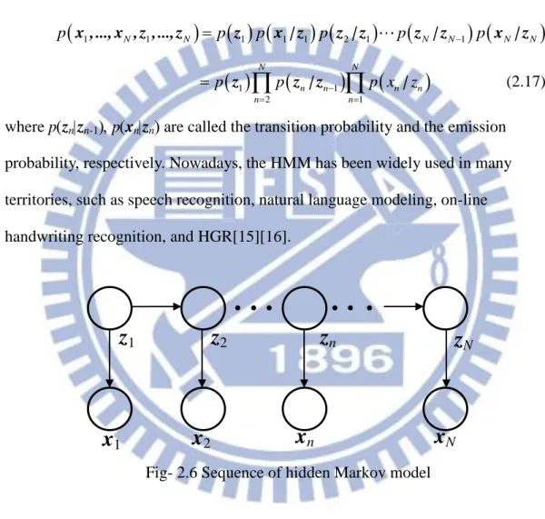
2 1 z z | z | N N n n n n n n p p _ p x z   



(2.17)

where pznzn-1pxnznare called the transition probability andthe emission probability, respectively. Nowadays, the HMM has been widely used in many territories, such as speech recognition, natural language modeling, on-line handwriting recognition, and HGR[15][16].

In real-time applications, there are two problems that must be solved for the use of HMM in (2.17) listed as below:

Problem1: Given N observations X{x1 ,..., xN} and all the model parameters pz1pznzn-1and pxnzn, for n1,...,N, how to compute the

posterior probability of each latent variable, p(znX)?

Problem2: Given N observations X {x1 ,..., xN}, how to estimate the parameters

x1

Fig- 2.6 Sequence of hidden Markov model

x

2

x

n

x

N

(26)

16

pz1pznzn-1and pxnznfor n1,...,N?

For the first problem, given the observations and all model parameters, (2.17) can be obtained and use the property described below:



|





,



p Z X  p Z X (2.18)

where X { x1 ,..., xN} and Z{ z1 ,..., zN}. Using the probability sum rule, the

posterior can be intuitively calculated as:













1 1 1 1 z z z z z | z , z , ..., z , n n N n n N p X p X p X    

  

(2.19)

for n1,...,N. It's an intuitive way to find the posterior probability, but it would need a vary large-scale computation time. Assume each latent variable zn is M-state discrete

random variable, (2.19) would need N-1 times of M summation calculation and the computation order is O(M N-1)! Due to this reason, a more efficient approach, the forward-backward algorithm[17] is used to reduce the computation time and the detail derivation is described in Appendix. A. To further speed up the calculation, the Viterbi algorithm is proposed that finding the most probable sequence of latent variables for a given observations X { x1 ,..., xN}. These two methods are based on the well-known

model parameters, but in real applications, these parameters are unknown and should be proper estimated given observations.

Problem 2 is a more difficult than previous since it need to determine a method to adjust the model parameters such that the likelihood function of the observations given model parameters, p(X|), where is model parameter, is maximum. However, given any observation sequence as training data, there's no close-form solution for estimating model parameters. Instead, an iterative procedure known as Baum-Welch method[18] or expectation-maximization (EM) algorithm is used to maximize the

(27)

17

likelihood function and obtain optimal parameters. Different initial values for the parameters would cause different result, so an suitable initial guess for these values is an important step when using EM algorithm.

(28)

18

Chapter 3 Hand Gesture Recognition System

3.1 Hand Region Detection

It's important to detect the exact hand region in real-time applications. A number of research has been proposed to extract the hand region precisely, such as the Adaboost learning algorithm [16] and SIFT features [17], but the cost of the computation time make it hard to implement on the real-time detection system. Since the extraction of skin color regions is fast, this method is usually used in hand detection even though it is very sensitive to lighting conditions. Based on skin region, the system could implement ROI selection with connected component labeling (CCL) to increase detection rate. To further distinguish the hand and face regions, the scheme proposed in [19] is adopted.

3.1.1 Skin Color Extraction

With the use of Kinect, a suitable distance range from the user to the screen can be selected and the depth information with lower value implies a smaller distance. Besides, all the points are offset to 0 if the sensor is not able to measure their depth. In our proposed remote hand-gesture control system, it is required that the hands move in the range around 0.5m to 2.0m. There are many skin color extraction methods which have been described in Chapter 2.2. To speed up the processing, we use a look-up-table method in YCbCr color space and the result is shown in Fig- 3.1. There are still a lot of noise pixels in skin color, so a method to remove them is required. As observed, these noise pixels usually have a small region comparing with the hand and

(29)

19

face regions, and thus can be removed by the connected component labeling (CCL) method.

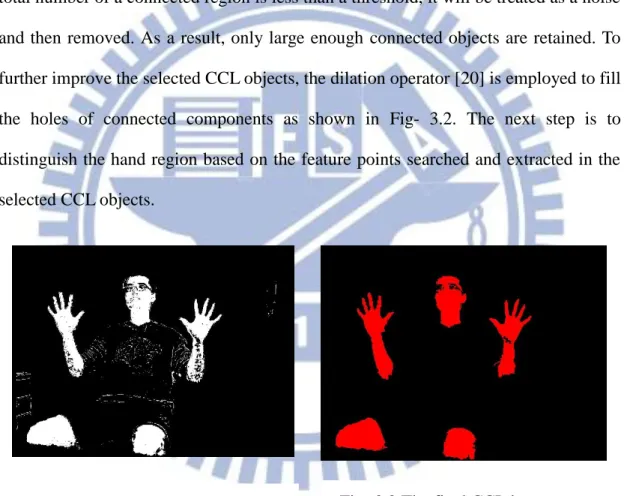
Connected Component Labeling (CCL) [20] is a technique to identify different components and often used to detect connected regions in binary images. This thesis applies a 4-pixel connected component to label interesting regions. Furthermore, in addition to recognizing the connected regions, CCL also compute their areas. If the total number of a connected region is less than a threshold, it will be treated as a noise and then removed. As a result, only large enough connected objects are retained. To further improve the selected CCL objects, the dilation operator [20] is employed to fill the holes of connected components as shown in Fig- 3.2. The next step is to distinguish the hand region based on the feature points searched and extracted in the selected CCL objects.

3.1.2 Feature Points Extraction

There are many distance transformation (DT) algorithms to transform a binary image into a distance images, which are different in the way distances are computed

(30)

20

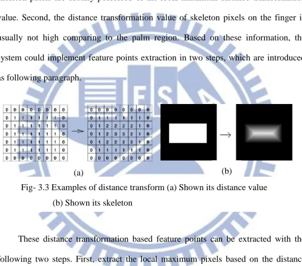
[21,22]. In this thesis, two-passed scanning distance transform is used in a binary image for its simplicity and efficiency in calculation, Fig- 3.3(a) given an example. To extract the feature points of distance transform image, a useful characteristics has been introduced in [19] based on two important qualities. First, the skeleton of an object can be extracted by distance transformation, as shown in Fig- 3.3(b), where the skeleton pixels are usually possessed of the local maximum distance transformation value. Second, the distance transformation value of skeleton pixels on the finger is usually not high comparing to the palm region. Based on these information, the system could implement feature points extraction in two steps, which are introduced as following paragraph.

These distance transformation based feature points can be extracted with the following two steps. First, extract the local maximum pixels based on the distance transformation value. On the distance transformation image, a local maximum pixel would satisfy the following condition:





1 , , i j G x i y  j 



(3.1)

where i,j 1,0,1and the function G is defined as:





1 if

 





0 otherwise , , , D x y D x i y j G x i y  j       (3.2)

Fig- 3.3 Examples of distance transform (a) Shown its distance value (b) Shown its skeleton

(31)

21

where D(x,y) is the distance transformation value at point (x,y). This condition implies that D(x,y) of the point at (x,y) is greater than or equal to those of its 8 neighborhood pixels, and thus a set of local maximum pixels can be extracted accordingly from the distance transformation image.

Second, determine the feature points from the set of local maximum points. In Fig- 3.4, the red-labeled pixels represent the extracted local maximum points. It can be found that those in the middle regions of the palm and arm have bigger D(x,y) from 20 to 50, so are those in the face. While along the contour, the pixels usually possess much lower D(x,y) from 2 to 5. For the local maximum pixels around the finger region, they have the middle distance transformation value satisfying the following condition:

 

10DV x y, 3 (3.3)

Significantly, (3.3) can be used as the condition to extracted the feature points which potentially contain the desired finger region. Fig- 3.5 also shows the extracted feature points, in blue. As shown in Fig- 3.5, we have found out the set of the feature points

Fig- 3.4 The local maximum distance-based feature pixels in different regions

(32)

22

still occurs in the wrist and face regions, so the depth information is used to detect the hand region.

3.1.3 Hand Classifier

After several experiment, we have found two important facts: First, under the same depth value, the total number of feature points on the face or other noise region is usually smaller than that on the open hand. Therefore, with the same number of contour, the hand region would have more feature points than that on face. Second, the total number of feature points is effected by the depth value. Due to these two observations, the relationship between the depth and FPs ratio(feature point number/total contour number) is needed and shown in Fig- 3.6, where the 1873 red crosses indicate the region only contain hand and the 1252 green crosses would contain the part of the forearm. The x-axis is the total feature points of the connected component divided by the total contour number while the y-axis is the mean depth of the object. To enhance the processing speed, a Gaussian likelihood model for hand detection is used for this thesis. This model makes the distribution of the hand as a 2-d Gaussian, and the model parameter can be found using the collecting hand training

(33)

23

data. This method provides an intuitive way to determine the similarity between input CCL object and the hand training data.

To determine connected component object is hand or not, the probability distribution of the hand is defined as follows:













1 2 1 1 1 2 2 x x μ_k T x μ_k p | C exp | |     _ _ _ _     _  _ _   (3.4)

where x x1 x2T,and x1 is the FPs ratio and x2 is the mean depth of the connected

component object and C indicates the hand class. The two parametersΣ andμ is covariance matrix and mean vector. Assume the training data are i.i.d., and the likelihood function can be found as below:







x_n



n

p X | C



p | C (3.5)

where X is the training data set. Use the maximum likelihood estimation, these two parameters can be obtained and shown as below:

(34)

24 1 μ x_j j N 



(3.6)







1 x_j μ x_j μ T j N  



  (3.7)

where Ndenotes the total number of training data. The CCL object is classified as hand when (3.4) is granter than a threshold The choice of value is a trade-off between the true and false positives, and the ROC curve via different is shown in Fig- 3.7. The result shows that the true positive rate can reach 95% while the false probability is less than 1%. To further avoid the false alarm situation, a CCL object is detected as hand when satisfies the following condition:

1 1 M m m HF  





where HFm indicates the hand detection flag at time sequence m and the function is

defined as:





1 if 0 otherwise x_m m p | C HF     (3.9)

The bigger M would cause a lower false alarm detection but slower down the processing speed. To reach a real-time HCI, M is chosen to be 8 in this thesis that meets both accuracy and processing speed requirements. The detection results shows in Fig- 3.8, where the green rectangle is the selected ROI region. Under a indoor lighting environment, there are not much noises appeared on the detected image and performs very fast. But some errors occur when there are overlaps between the hand and the other skin color object, like face and skin color suits shown as Fig- 3.9. To overcome this problem, a refining process is proposed using the depth distribution information.

(35)

25

3.1.4 Depth Cutting

Some miss detection situation happens when there is a overlapping problem since the CCL algorithm would take the whole connected skin region as a same component. In general, two different skin color object exist in two different depth plane, so a hand detection processing under different depth level can be used to

Fig- 3.9 The miss detected results where the hand and (a) face (b) skin color suits are overlapping.

(a) (b)

Fig- 3.7 ROC curve under different threshold

(36)

26

separate these objects. Based on the depth information of skin color image, the system could implement histogram in three steps, which are introduced as following:

Step 1:After a skin-color extraction on whole image, first use CCL algorithm to filter out the skin color noise which has small area of connected points. This step clear out the small skin color background of the whole depth level.

Step 2:The system computes the depth histogram of the skin color image where the intensity levels is on the range [0, 255], where Fig- 3.10 shows the example. The depth distribution of Fig- 3.10 (b) is shown as Fig- 3.10 (c), which can be divided into two clusters: one is the right hand part that close to the camera; the other is face and the left hand regions. Let the depth histogram of the skin color image be:



1 255



h h h (3.10)

where hi is histogram number related to intensity i, i1~255. The k-th depth

region cutting would satisfy the following condition:

1 k k U j j L h  



(3.11)

where Lk and Uk indicate the lower and upper bound of k-th depth cutting

region, respectively. With the aid of the cutting region, we can process skin color detection and CCL operation corresponding to different cutting region such that the overlapping skin color regions can be separated.

(37)

27

Step 3:Assume there are K depth searching regions, the selected depth search level is determined by the following algorithm:









1 2 7 7 k k k k k k k k for k ~ K if U L continue; else if L U Search Level L ,L ; else Search Level L ,U ; end        

This algorithm stats that we will skip searching when the depth continuous distribution region is too small, and the maximum depth search interval is 7 since the hand is usually the closest object to the camera. The system then implements the feature points extraction and hand classifier respect to different depth cutting regions. Using the refining step can solve this overlapping problem and the Fig- 3.11 shows the result.

Fig- 3.10 (a) The original image. (b) The skin color region after CCL thresholding (c) Depth histogram of image.

(a)

(b)

(38)

28

Using the depth cutting refining can overcome the overlapping problem, and once it has been detected, the searching region is determined around the depth of the detected hand. However, the detected hand region still include the forearm part, which is not helpful for the HGR. So the next step is the forearm cropped procedure and find useful hand features to further increase the processing speed.

Fig- 3.11 The correct detection result even when hand and face are overlapping.

(39)

29

3.2 Hand Feature Extraction

After hand region detection, the system has to extract useful features to increase the detection rate and decrease the computational cost. Based on the distance-based feature points extracted from the previous section, a hand feature with the center of the palm, the hand direction and the five fingertip positions can be extracted fast and precisely. These features are very important parameters for both gesture recognition and hand tracking.

3.2.1 Hand Direction and Hand Region

The direction of the hand is an important cue for recognition. With the usage of the feature point and the binary hand region, this feature can be obtained in these two steps. First, the CCL center can be obtained by calculating the central moment on a binary segmented hand image I(x,y), where the I(x,y)Then the center point (xCCLMean , yCCLMean) can be determined using:

 

, , , , , , , , , x x y x x y mean mean x y x y x I x y y I x y x y I x y I x y 

 



 



(3.12)

Second, using the same equation (3.12), calculate the feature points mean, denote as (xFPMean , yFPMean). The direction is the line the connects the hand center and feature

points mean, and the degree of the hand direction is determined by using the following function: 2 CCLMean FPMean CCLMean FPMean y y HD arctan x x      _ _    (3.13)

where arctan2 function returns the positive angle for counter-clockwise angles (upper half-plane, y > 0), and negative for clockwise angles (lower half-plane, y < 0). Fig-

(40)

30

3.12 shows the result, where the blue, green, and black pixels are feature points, feature mean point, and CCL center, respectively. These figures show that even through the CCL object contains the forearm part, the hand direction can be extracted precisely. The next step is to exclude the forearm region from the CCL object.

Obviously, if the object is farer from the camera, the object would have smaller size in the image. Therefore, the detected hand size would be influenced by different distances. The relation between the size of the hand in the image and the distance from object to camera as shown in Fig- 3.13, where x-axis is the width of the hand and y-axis is the corresponding depth value. Due to this characteristic, the hand size can be modeled as a linear function of the depth value shown as below:

W   a Depth b (3.14)

where a,b are positive parameters. The hand region can be obtained in two steps. First, determine two points (xd,yd) and (xp,yp) on the hand direction line and satisfy the

following conditions: the distance from (xFPMean , yFPMean) to point (xd,yd) is 0.45 times

the hand width W, and the point is on the same side of the hand direction, while point (xp,yp) is 0.55W and on the opposite side of hand direction. Consequently , (xd,yd) and

(xp,yp) can be calculated as below:

Fig- 3.12 The hand direction (a) without forearm (b) with forearm.

(41)

31









0 45 0 45 d FPMean d FPMean x x . W cos HD y y . W sin HD           (3.15)









0 55 0 55 p FPMean p FPMean x x . W cos HD y y . W sin HD           (3.16)

Therefore, the hand direction line can be determined by the two points. Second, determine a line passing through (xp,yp) with length W and is perpendicular to the

hand direction. This line is near the wrist which can be used to separate the fingers and palm from the wrist and arm as Fig- 3.14. These two lines can determine a rectangle region that excludes the forearm region shown in Fig- 3.15, where the green rectangle is the CCL region and blue one is selected hand region. Therefore, the palm center, (xcenter,ycenter), can be determined by calculating the mean point within the blue

rectangle area.

The process above usually takes a little time since the total number of distance-based feature points is usually small. The next step is to search the fingertips location.

Fig- 3.13 The hand size under different depth value

Fig- 3.14 The process separating the forearm part.

(42)

32

3.2.2 Fingertip Positions

As shown in Section 3.1.2, there are many feature points in the fingertips region, and these points can be used to determine the fingertips position quickly and accurately. Fig- 3.16 (a) shows the detected hand region, where red pixels are the skin color and blue pixels are feature points, and the fingertips position can be found by the following steps.

Step1: Extract the feature points in Fig- 3.16 (a), shown as Fig- 3.16 (b), and then implement dilation operation to connect the discontinuous feature points, and the result shown as Fig- 3.16 (c).

Step2: Use CCL to label connected region and compute each CCL region. Only larger enough CCL area is considered as fingers, and the area is related to the distance from camera to the hand. Fig- 3.17 shows the average connected region of finger corresponding to different depth value. The other CCL region which is less than one deviation value would be taken as noise, and the Fig- 3.16 (c) shows the result.

Fig- 3.15 The result finding hand region (a) without forearm part (b) with forearm.

(43)

33

Step3: Calculate the mean and standard deviation of each CCL object, and two candidate fingertip positions, CTi,1 and CTi,2, i=1~5, can be calculated, shown

as Fig- 3.16(d). Calculate the distance between the candidate fingertip and wrist line, which is obtained by Chapter 3.2.1. The point which is far from the wrist line is the selected fingertip position, and the result shown in Fig- 3.16(e). And the fingertip angle is the connection from CTi,1 and CTi,2.

With the proposed method, the hand feature extraction process will determined the all outstretched hand direction, fingertip positions and the palm center. Once these features are obtained, the recognition system can grasp the posture of the hand more easily, and the hand tracking process can be also performed more easily and precisely.

Fig- 3.16 The procedure of finding fingertips position (a) detected hand region (b) the feature points (c) implement dilation (d) mean and standard deviation corresponding to each CCL object (e) the selected fingertips.

(a)

(d)

(b) (c)

(44)

34 In detail, the set of the features includes: 1. The position of palm center, (xcenter,ycenter).

2. The displacement of palm center. 3. The hand direction, HD。.

4. Total detected fingertips number and its positions.(from 1 to 5). 5. Direction of each finger.

6. The depth mean of the hand. 7. The change of the mean depth.

8. The mean distance from (xcenter,ycenter) to each fingertip.

From the above hand features, a hand recognition model can be built. Moreover, these features can be exploited not only by HGR system but also by hand tracking system.

(45)

35

3.3 Hand Gesture Recognition

After hand region detection, the system has to judge recognize different gestures based on the extracted features. To test the ability of variation tolerance, both sequential and non-sequential training method. This thesis adopts discriminative classification model, neuron network and hidden Markov model to implement the HGR systems. The features which are extracted in chapter 3.2 are sent into these HGR systems and compare their recognition rate and processing speed. The resolution in the experiments are 640×480 at 20 frames-per second. These approaches would be introduced below and their performances would be compared in Chapter 4. This experiment test 6 hand gestures to be recognized, including moving left, right, upward, downward, open and click.

3.3.1 Discriminative Model

The discriminative model directly assume the posterior probability of class Ck

as a logistic sigmoid acting on a linear function of the input vectors:





 





 

1 1 1 1 exp | , 1 ~ 1 1 exp 1 | 1 exp j k k T j K T k K K T k p C j K p C       _ _  _       



w x x w x x w x (3.17)

where x is input vector and w is the weighting vector. Given the data set {xn,tn}, n=1~N, where tntn,1 tn,2... tn,K-1 and tn,k1 when xn belongs to class k while the

others are 0,the likelihood function can be written as below:





, 1 1 1 , 1 1 |w ,...,w n k N K t K n k n k p T y     



(3.18)

(46)

36

logarithm of (3.18), which gives the cross-entropy function in the following form:



1 1



1 , , 1 1 ,..., ln w w N K K n k n k n k E t y      



(3.19)

The error function can be minimized by the Newton-Raphson iterative optimization method, which uses a local quadratic approximation to the log likelihood function. The Newton-Raphson update for minimizing error function takes the following form:

 

1

Wnew Wold W

H E

   (3.20)

where W=[w1 w2... wK-1]T is the whole weighting vector and H is the Hessian matrix

whose elements contain the second derivatives of E(W) with respect to each wj. The

each component of the gradient is given as below:

 

W w₁

 

W w₂

 

W w_K₁

 

W T E  E E _E    _   _ (3.21) where

 



, ,



1 W x j N w n j n j n n E y t   



 (3.22)

The each component of Hessian matrix is computed using the following:

 

1 1 1 1 1 1 1 1 w w w w w w w w W W W W K K K K E E H E E                 _ _ _ _    (3.23) where

 

,



, ,



1 w_k w_j W I x x_n N T n k k j n j n n E y y     



 (3.24)

The Hessian matrix for the multiclass classification problem is positive definite and the error function can converge to a unique minimum. In this thesis, K is chosen to be 6 to recognize the defined gestures.

3.3.2 Neural-Network-Based Recognition

(47)

37

layer with O neurons, one hidden layer with P neurons, and one output layer with Q neuron. After feature extraction, these features are sent into the neural network as inputs. The O neurons of the input layer are represented by x. The i-th input neuron is connected to the j-th neuron, j1,2,…,P, of the hidden layer with weighting wj(1).

Besides, the j-th neuron of the hidden layer is also with an extra bias wj0(1). Finally, the j-th neuron of the hidden layer is connected to k-th output neuron with weighting wk(2), k=1,2,…,Q, and a bias wk0(1) is added to the output neuron.

Let the activation function of the hidden layer be the hyperbolic tangent-sigmoid transfer function and the output vector of hidden layer is expressed as

1 2 [z z zP]T  z (3.25) where

















(1) (1) (1) (1) exp exp , 1, 2,..., exp exp T T j j j _T _T j j z     j P    w x w x w x w x (3.26)

Let the activation function of the output layer be the softmax function and the output is expressed as 1 2 [y y y_Q]T  y (3.27) where









(2) 1 (2) 1 1 1 exp , 1, 2,..., 1 1 exp 1 T k k Q T k k Q Q k k y k Q y y           _     _{ } 



w z w z (3.28)

The above operations are shown in Fig- 3.18. The weights of neural network would be adjusted through the process of back-propagation learning algorithm. After learning, the HGR system can be recognized according to the output value of neural network.

(48)

38

The final recognition result is made using the following decision strategy: arg max _q, 1, 2,...,

q

HG y q Q (3.29)

In this experiment, the number of neuron in each layer are 8, 10, 6 corresponding to input, hidden, and output layer.

3.3.3 HMM-Based Recognition

As a hand gesture is basically an action composed of a sequence of hand postures that are connected by continuous motions, thus describing the hand gestures in terms of a sequential input is suitable in HGR systems. HMM have been applied to HGR tasks with success. The classification of the input sequence proceeds by computing the sequence's similarity to each of the gesture class models. The joint distribution is given by:

1

x

1

x

O 1

z

P

_y

Q

y

1 kK

z

1

Fig- 3.18 HGR ANN structure

┼ ┼ WS1(p,q) S(p) bS1 (q) WS2 (q) bS2 x + x +

(49)

39



1 1



 

1



1







2 1 N N N N n n n n n n p p p _ p x z   



x , ..., x , z , ..., z z z | z | (3.30)

where pznzn-1pxnznare called transition andemission probability, respectively. zn

is the latent variable, or called hidden state, corresponding to the input data xn. An

iterative expectation-maximization (EM) algorithm procedure is used to maximize the likelihood function and obtain optimal parameters. To speed up the calculation, the Viterbi algorithm is used that finding the most probable sequence of latent variables for a given observations X {x1 ,..., xN}. The posterior probability of time t is

proportional to the jointly probability:

1 1 1 1 ( ,..., _t| ,..., _t) ( ,..., , ,...,_t _t)

p z z x x  p z z x x (3.31)

Let z1,...,zt≡z1:t and x1,...,xt≡x1:t, and the message passed in the max-sum algorithm

are given by:

1 1 1 1 2 1 1: 1: ,..., 1 1: 1 1: 1 ,..., 1 1 ( ) max ( , ) = max[ ( | ) ( | ) max ( , )] = max[ ( | ) ( | ) ( )] t t t t t t t z z t t t t t t z z z t t t t t z z p z x p x z p z z p z x p x z p z z z            (3.32)

The Viterbi algorithm consider explicitly all of the exponentially many paths, evaluate the probability for each and then select the path having the highest probability. In this experiment, the latent variable zn has 6 states and N is chosen to be 10.

This experiment test 6 hand gestures to be recognized, including moving left, right, upward, downward, open and click, and Fig- 3-19 shows the defined gestures. The hand gestures are defined in natural way rather than in particular ordered hand pose. The palm center difference between the current and previous frames can be used to recognize the these gestures. The above three algorithms are used to recognize these six hand gestures.

(50)

40 Fig- 3.19 The defined hand gestures.

(51)

41

Chapter 4 Experimental Results

In the previous chapters, the three main steps of the proposed HGR system are introduced. In this chapter, the experiment results of each step will be shown in detail and the results of the proposed algorithm will be obtained by MATLAB R2010b and OpenCV 2.2.

4.1 Hand Region Detection

To examine the reliability of hand region detection, the system is tested in many different situations, including different distances, the skin color background, overlapping by other skin object and more than one human, and the results are shown from Fig- 4.1 to Fig- 4.4, respectively. The left column contains the skin color images, the middle one shows the ROI images, and the right one represents the skin color regions with large enough area, where the white pixel indicates skin color and red represents the depth searching region. Note that the green rectangles in the middle are the selected ROIs. Fig- 4.1 shows even though human keeps moving away from the camera, the system would not fail to extract hand region. The distance between the human and camera is from 0.5m to 2m. In Fig-4.2, there are some skin color objects

in the images, and the system also could detect the hand

(52)

42

(b) (c)

Fig- 4.1 Results of hand region detection in different distances. (a) The original skin color region (b) The ROI images (c) skin color regions with large enough area. Note that the green rectangles in (b) are the selected ROIs.

基於影像特徵點擷取結合深度資訊之 即時手勢辨識系統設計

國 立 交 通 大 學

電控工程研究所

碩 士 論 文