利用有視覺自動車作室內安全巡邏與危險情況之偵測

國

立

交

通

大

學

資訊科學與工程研究所

碩

士

論

文

利用有視覺自動車作室內安全巡邏與危險

情況之偵測

Security Patrolling and Danger Condition Monitoring in

Indoor Environments by Vision-based Autonomous

Vehicle Navigation

研 究 生：江凱立

指導教授：蔡文祥 教授

利用有視覺自動車作室內安全巡邏與危險情況之偵測

Security Patrolling and Danger Condition Monitoring in Indoor

Environments by Vision-based Autonomous Vehicle Navigation

研 究 生：江凱立 Student：Kai-Li Chiang

指導教授：蔡文祥 Advisor：Wen-Hsiang Tsai

國 立 交 通 大 學

資 訊 科 學 與 工 程 研 究 所

碩 士 論 文

A Thesis

Submitted to Institute of Computer Science and Engineering College of Computer Science

National Chiao Tung University in partial Fulfillment of the Requirements

for the Degree of Master

In

Computer Science June 2006

Hsinchu, Taiwan, Republic of China

利用有視覺自動車作室內安全巡邏與危險情況之偵測

研究生：江凱立

指導教授：蔡文祥 博士

國立交通大學資訊科學與工程研究所

摘要

本研究主要是提出一套基於電腦視覺技術，讓自動車航行在室內環境中具有 偵測危險情況與監控繪畫安全之能力。我們利用一台小型自動車作為實驗平台， 並且利用無線操控的方式讓自動車航行在室內的環境中。我們提出了基於房屋中 天花板角落的自動車定位方式，根據天花板角落的線條形成情況我們可以計算自 動車在地圖上的實際位置。我們持續觀察環境影像並統計環境中的顏色特徵與連 續影像的顏色變化，來判斷目前的環境情況是否安全。依據環境中的顏色統計資 訊與變化情況，我們可以偵測出火災發生或環境停電。我們利用觀察影像中的限 定區域，判斷是否遇到障礙物，以順利避開障礙物繼續巡邏。對於牆壁上的掛畫， 我們提出一套將歪斜影像修復的方法來得到正確的掛畫影像，並基於此修正過的 掛畫影像進行保全掛畫之安全巡邏。最後我們以成功的定位和偵測環境實驗結果 證明本系統的完整性與可行性。

Security Patrolling and Danger Condition Monitoring

in Indoor Environments by Vision-based

Autonomous Vehicle Navigation

Student: Kai-Li Chiang

Advisor: Wen-Hsiang Tsai

Institute of Computer Science and Engineering

National Chiao Tung University

ABSTRACT

A vision-based vehicle system for security patrolling and danger condition monitoring in indoor environments using an autonomous vehicle is proposed. A small vehicle with wireless control and image grabbing capabilities is used as a test bed. A camera with panning, tilting, and zooming capabilities is used as the eye of the small vehicle. A vehicle location estimation method using house corners is proposed first. This is a vision-based estimation method to prevent the mechanic error accumulation in navigation. Next, several danger condition detection methods are proposed. We propose a method to change the path for obstacle avoidance in navigation using a map of nodes. To detect fire and lighting failure conditions, we monitor the image continuously and analyze the color feature in the HSI color model. We have also proposed a method for security monitoring of paintings on walls, including techniques of painting image rectification and matching. Good experimental results show flexibility and feasibility of the proposed methods for the application of indoor security patrolling.

ACKNOWLEDGEMENTS

I am in hearty appreciation of the continuous guidance, discussions, support, and encouragement received from my advisor, Dr. Wen-Hsiang Tsai, not only in the development of this thesis, but also in every aspect of my personal growth.

Thanks are due to Mr. Tsung-Yuan Liu, Mr. Chih-Jen Wu, Miss. Pei-Pei Chen, Mr. Yen-Long Chen, Mr. Kuo-Feng Chien, Miss Yu-Tzu Wang, Miss Chia-Yu Hsu, and Miss Yi-Lin Wang for their valuable discussions, suggestions, and encouragement. Appreciation is also given to the colleagues of the Computer Vision Laboratory in the Institute of Computer Science and Engineering at National Chiao Tung University for their suggestions and help during my thesis study.

Finally, I also extend my profound thanks to my family for their lasting love, care, and encouragement. I dedicate this dissertation to my beloved parents and girlfriend.

CONTENTS

ABSTRACT (in Chinese) ... I

ABSTRACT (in English) ...II

ACKNOWLEDGEMENTS ... III

CONTENTS ... IV

LIST OF FIGURES ...VII

Chapter 1

Introduction ...1

1.1 Motivation ...1

1.2 Survey of Related Studies ...2

1.3 Overview of Proposed Approach ...3

1.4 Contributions ...5

1.5 Thesis Organization ...6

Chapter 2

System Configuration and Navigation

Principles ...7

2.1 Overview 7... 2.2 Advantage of Using Pan-tilt-zoom IP Cameras ...8

2.3 System Configuration ...9

2.3.1 Hardware Configuration ...9

2.3.2 Software Configuration ...13

2.4 Vehicle Guidance Principle ...13

Chapter 3

Vehicle Guidance by Vehicle Location

Estimation Using A House Corner

Detection Technique ...16

3.2 Review of Vehicle Location Estimation Techniques ... 17

3.3 Vehicle Location Estimation by House Corner Detection ...19

3.3.1 Coordinate Systems ...20

3.3.2 Principle of Proposed Method ...21

3.3.3 Location Estimation by Coefficients of Edge Line Equations ...22

3.4 Image Processing for Vehicle Location Estimation ...26

3.4.1 Detection of House Corner Edges ...27

3.4.2 Constrained Line Refitting and Determination of Non-vertical House Corner Edges ...31

Chapter 4

Obstacle Avoidance by Goal-Directed

Minimum-Path Following ...40

4.1 Overview of Obstacle Avoidance ...40

4.1.1 Coordinate Systems ...42

4.1.2 Direction Angle of Vehicle ...43

4.1.3 Coordinate Transformation ...44

4.2 Obstacle Detection Process ...44

4.2.1 Finding Floor Area ...46

4.2.2 Determination of Obstacle Existence ...47

4.3 Minimum-Path Following Process ...49

4.3.1 Detection of Obstacle Distribution ...49

4.3.2 Computation of Goal-Direction Minimum Path ...51

Chapter 5

Vision-Based Indoor Danger Condition

Monitoring ...56

5.1 Principle of Danger Condition Monitoring ...56

5.2 Advantage of Using HSI Color Model ...57

5.3 Dangerous Fire Condition ...59

5.3.1 Fire Image Features ...59

5.3.2 Proposed Fire Detection Method ...60

5.4 Lighting Failure Condition ...64

5.4.1 Lighting Failure Features ...64

5.4.2 Process for Lighting Failure Detection ...65

Chapter 6

Security Monitoring of Paintings on Walls

Rectification Technique ...70

6.1 Overview ...70

6.2 Rectification of Images of Paintings on Walls ...71

6.2.1 Difference Between Images of Paintings on Walls And Objects on Floors ...71

6.2.2 Rectification of Skewed Images ...72

6.3 Security Monitoring of Paintings on Walls by Image Analysis ...75

6.3.1 Painting Image Features ...75

6.3.2 Learning Process ...76

6.3.3 Painting Security Monitoring Process ...82

Chapter 7

Experimental Results and Discussion ....89

Chapter 8

Conclusions and Suggestions for Future

Works ...94

8.1 Conclusions ...94

8.2 Suggestions for Future Works ...95

LIST

OF

FIGURES

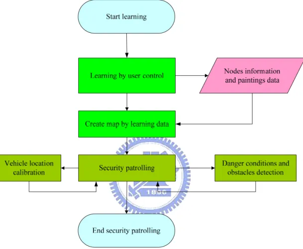
Figure 1.1 Flowchart of proposed system...5

Figure 2.1 Action of a pan-tilt-zoom camera. ...9

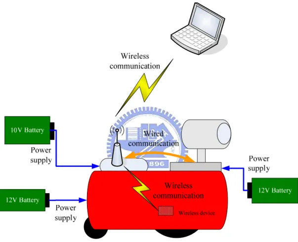
Figure 2.2 Structure of the system ...10

Figure 2.3 The vehicle used in this study. (a) The bevel view of the vehicle. (b) The front view of the vehicle. (c) The left side view of the vehicle. ... 11

Figure 2.4 The pan-tilt-zoom camera used in this study. (a) The bevel view of the camera. (b) The front view of the camera. (c) The right side view of the camera. ...12

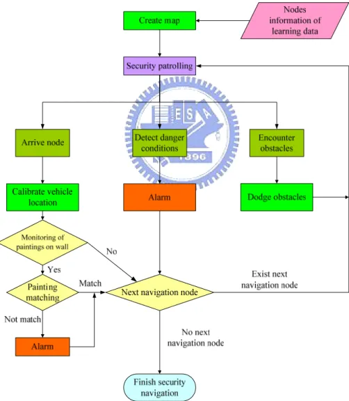
Figure 2.5 Flowchart of proposed navigation process ...14

Figure 3.1 Three different landmarks. (a) A diamond-shaped standard mark used in [6]. (b) A sphere used for robot location in [7]. (c) The perspective projection of a house corner used in Chou and Tsai [8]...18

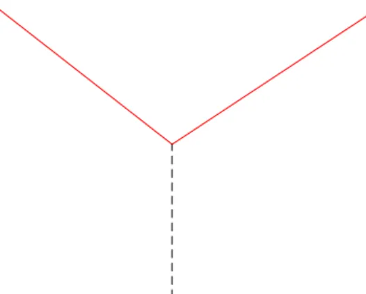
Figure 3.2 The two red lines of the perspective projection of a house corner used in the study. ...20

Figure 3.3 The three coordinate systems used in this study...21

Figure 3.4 Flowchart of vehicle location estimation. ...27

Figure 3.5 Flowchart of house corner edges detection ...27

Figure 3.6 (a) The color corner images. (b) The Canny result images of (a). ...28

Figure 3.7 The image after applying Hough transform in Figure 3.6 (b). ...29

Figure 3.8 An experimental result of a different house corner. (a) Another corner image. (b) The result of applying Canny edge detection of (a). The result of applying Hough transform of (b)...30

Figure 3.9 One more experimental result of another different house corner. (a) Another corner image. (b) The result of applying Canny edge detection of (a). The result of applying Hough transform of (b). ...31

Figure 3.10 Flowchart of the coefficients of corner edge equation computation. ...32

Figure 3.11 Illustration of a set of lines representing an identical house corner edge. 33 Figure 3.12 The house corner center of an house corner image. ...34

Figure 3.13 The different color points represent the different edge respectively. ...35

Figure 3.14 Refitting of two non-vertical corner edges...37

Figure 3.15 An experimental result of a different house corner. (a) The sets of lines represent an identical house corner edge. (b) The house corner center. (c) The edge points (d) Refitting of two non-vertical corner edges ...38

Figure 3.16 One more experimental result of another different house corner. (a) The sets of lines represent an identical house corner edge. (b) The house corner center. (c) The edge points (d) Refitting of two non-vertical corner edges39 Figure 4.1 Flowchart of obstacle avoidance process. ...41 Figure 4.2 Two coordinate systems in this study. (a) The vehicle coordinate system. (b)

The global coordinate system. ...42 Figure 4.3 Definition of the direction angle (a) ω is positive. (b) ω is negative. ...43 Figure 4.4 The coordinate transformation between the vehicle coordinate system and

vehicle coordinate system. ...44 Figure 4.5 Flowchart of obstacle detection process...45 Figure 4.6 Region growing to find the floor area in an image. (a) The floor image. (b)

Detection of the floor area. ...47 Figure 4.7 Detection of an obstacle within the warning area. (a) An image including

an obstacle. (b) The detection of the obstacle...49 Figure 4.8 An illustrated of attaching the lines on the floor...50 Figure 4.9 Using an obstacle image to find the front of the obstacle in the WCS. (a)

An obstacle in image coordinate system. (b) The front of the obstacle in world coordinate system. ...51 Figure 4.10 An illustration of computation of goal-direction minimum path...52 Figure 4.11 Top view of an obstacle avoidance experiment. ...54 Figure 5.1 RGB 24-bit color cube. (a) Cube with black corner. (c) Cube with white

corner [13]...57 Figure 5.2 The HSI color model based on circular color planes. The circles are

perpendicular to the vertical intensity axis [13]...58 Figure 5.3 Flowchart of fire detection. ...61 Figure 5.4 (a) An image without fire. (b) The hue of (a) within the ranges Hf1 or Hf2. (c)

The saturation of (a) over than Sf. (d) The intensity of (a) equals If. (e) The

intersection of (b), (c), (d), and (e)...62 Figure 5.5 (a) An image with fire. (b) The hue of (a) within the ranges Hf1 or Hf2. (c)

The saturation of (a) over than Sf. (d) The intensity of (a) equals If. (e) The

intersection of (b), (c), (d), and (e)...63 Figure 5.6 The two consecutive images in ordinary situation. ...65 Figure 5.7 The two consecutive images when the lighting fails. (a) The ordinary

image. (b) The image of lighting failure. ...65 Figure 5.8 The continuous images. (a) The initial situation. (b) The ordinary situation

after (a). (c) The image of the lighting failure. (d) The continuous image after (c)...67

Figure 5.9 The continuous images. (a) The initial situation. (b) The ordinary situation after (a). (c) The image of the lighting failure. (d) The continuous image

after (c)...68

Figure 5.10 The intensity histograms respective to Figure 5.X. (a) The mean of the intensity is 0.73. (b) The mean of the intensity is 0.73. (c) The mean of the intensity is 0.55. (d) The mean of the intensity is 0.32. ...68

Figure 5.11 Flowchart of lighting failure detection. ...69

Figure 6.1 A skewed image...72

Figure 6.2 A painting on a wall image. ...76

Figure 6.3 The flowchart of computation of the matrix H...79

Figure 6.4 The flowchart of the learning painting process. ...80

Figure 6.5 The experimental result of learning a painting. (a) A painting on a wall image. (b) A rectangle including the painting. (c) The four borders of the painting. (d) The four intersections computed from the four borders. (e) The four point correspondences. (f) The rectified painting. ...81

Figure 6.6 The flowchart of the painting matching process. ...84

Figure 6.7 The experimental results of the painting matching process. (a) and (b) are the two different rectified painting image of the same painting. (c) and (d) are the normalized image in gray-level of (a) and (b) respectively. (e) and (f) are the block image of (c) and (d) respectively. (g) is the overlapping result of (e) and (f). ...85

Figure 6.8 The experimental results of the painting matching process of two different paintings. (a) and (b) are the two different rectified painting image of the two different paintings. (c) and (d) are the normalized image in gray-level of (a) and (b) respectively. (e) and (f) are the block image of (c) and (d) respectively. (g) is the overlapping result of (e) and (f)...86

Figure 6.9 The flowchart of the security monitoring process. ...88

Figure 7.1 The used corner and learned image. ...89

Figure 7.2 An illustration of learned data and navigation path...90

Figure 7.3 A navigation process. (a) and (b) are ordinary situations. (c) and (d) are obstacle avoidance. (e) and (f) show the vehicle monitoring a painting. ..92

Figure 7.4 The experimental result of obstacle avoidance and detection of lighting failure and fire...92

Chapter 1

Introduction

1.1 Motivation

Researches on autonomous vehicles or mobile robots have been conducted for a long time, and there are more and more applications in this domain. Applications of vision-based vehicles are especially useful in human environments, such as nursing robots, entertainment robots, home service robots, security patrolling robots, etc.

For security surveillance, installation of stationary cameras is a usual method to monitor indoor environments. However, there may exist some areas the camera view cannot cover because the cameras are fixed. This is an obvious disadvantage of conventional security surveillance systems. Fortunately, we can employ a vision-based autonomous vehicle to overcome this weakness because the vehicle is movable. It can navigate around indoor environments to help monitor the areas the camera view cannot cover. Moreover, the use of vehicles has other advantages. For example, it can substitute manpower because a vehicle only spends electronic power or fuel, is able to patrol the whole day, and need not rest like human beings.

In most applications, we must take the advantage of learning to teach a vehicle where to navigate, what to monitor, and how to judge whether an object exists or not, before it starts security patrolling in indoor environments. After the learning process, the vehicle can navigate around the environment and monitor objects autonomously.

autonomous vehicle with capabilities of obstacle avoidance and danger condition detection is necessary in many applications. One of the research goals in this study is to develop a method to detect danger conditions, such as obstacles or fire, and make the vehicle possess the ability to avoid obstacles or to warn people of danger conditions.

With the improvement of the camera technology, a vehicle can be equipped with a pan-tilt-zoom camera (abbreviated as PTZ camera in the sequel) nowadays instead of with a fixed pinhole camera used in the past. Such vision-based autonomous vehicles can help human beings to complete more tasks. By means of the PTZ camera, the view of a vehicle is no longer restricted to be a lower area; instead, it is extended to a wider range. Thus we also propose an approach to monitoring paintings on walls using features in images taken with PTZ cameras.

1.2 Survey of Related Studies

In order to let a vehicle navigate automatically and complete the mission of security patrolling in indoor environments, the design of a learning strategy is required. The aim of this step is to learn navigation paths and to record the features of monitored objects. Furthermore, it is very important to know the distance between the vehicle and an object no matter in learning or navigation. A 2D-to-3D distance transformations proposed by Lai and Tsai [1] is to use a curve fitting technique and a modified interpolation technique. Then the distances between the vehicle and the surroundings in real world can be known through captured images. Li and Tsai [2] proposed a graph-based navigation method. The creation of a navigation map is also accomplished through a learning process. Then the vehicle navigates according to the

nodes in the map. The learning process adopted certain complex learning rules to help construct the map. Moreover, Chen and Tsai [3] proposed a fuzzy guidance technique in two navigation modes. It needs to take two kinds of learned data to create the navigation map. After creating the map, a fuzzy guidance technique is applied to accomplish the navigation work. Liu and Tsai [4] proposed a security patrolling navigation method which utilizes multiple-camera vision and autonomous vehicle navigation techniques to patrol in building corridors. Chen and Tsai [5] proposed a learning method by manual driving to teach the vehicle where to navigate and what to monitor. By this method, the vehicle has the ability to navigate in indoor environments and to monitor objects automatically after learning.

The vehicle location is very useful information in navigation, so we need a method to estimate the vehicle location. Installing an odometer on the vehicle is a good idea, but using a vision-based vehicle location estimation method is a better way to tolerate mechanic errors. Fukui [6] proposed a method to locate vehicle locations by placing diamond shapes whose boundary consists of four identical thick line segments with known lengths. Magee and Aggarwal [7] used a sphere on which two perpendicular great circles are drawn as a standard landmark for vehicle location. Chou and Tsai [8] proposed a method which utilized a house corner existing naturally in the house to estimate the vehicle location.

1.3 Overview of Proposed Approach

The aim of this study is to design a vision-based vehicle system for security surveillance in indoor environments with danger condition monitoring ability. An

purpose, the system needs not only an ability of navigation but also an ability to pay attention to surrounding environments. Furthermore, design of a simple and flexible learning method is also necessary. In order to achieve these two goals, we use two tools. One is an odometer in the vehicle and the other is the image captured by the camera equipped on the vehicle. The odometer provides the position of the vehicle, and the image helps recognition of objects and monitoring of surrounding environments. We also utilize images to detect house corner for the vehicle location estimation. The vehicle equipped a PTZ camera has the ability to monitor objects at a higher view, such as paintings on walls.

Since the vehicle is a kind of machine, records of the odometer in the vehicle may include mechanic errors after the vehicle navigates a sufficient distance. Calibration of the vehicle location is necessary to prevent the error from accumulating too seriously. We propose a vision-based vehicle location estimation method to adjust the position and direction of the vehicle. This method utilizes the image of a house corner.

The vehicle may also be designed to have the capability of observing surroundings all the time to detect danger conditions immediately. In order to detect danger conditions as soon as possible, a simpler and faster method is necessary. The HSI color of an image of the surrounding provides very good attributes to help the vehicle judge whether the surrounding condition is dangerous or not in real time. We use the camera to capture the surrounding image sequentially and analyze the conditions continuously.

The camera on the vehicle is normally equipped at a lower position. Therefore, when the camera is used to take an image of a higher view, the taken image is always skewed. In order to increase the accuracy of monitoring paintings on walls, we apply an image rectification technique to correct the image skewing. The shape and the ratio

features of a rectified image are more proper for use in security monitoring of paintings. It is necessary to carry out image rectification automatically when the vehicle performs security surveillance. We use the features of paintings on walls and some image processing techniques to obtain rectified images of paintings.

Figure 1.1 Flowchart of proposed system.

1.4 Contributions

The main contributions of this study are summarized in the following.

(1) A vision-based vehicle location estimation method utilizing house corner images to prevent mechanic errors from accumulation is proposed.

camera is proposed.

(3) A faster and simpler and less method for real-time obstacle avoidance by goal-directed minimum path following is proposed.

(4) A method for detecting dangerous fire and lighting failure conditions during security surveillance navigation is proposed.

(5) An image rectification technique for paintings on walls is proposed. (6) A method for security monitoring of paintings on walls is proposed.

(7) A method for detecting and recognizing paintings on walls automatically using the Hough line transform is proposed.

1.5 Thesis Organization

The remainder of this thesis is organized as follows. In Chapter 2, we describe the system configuration of the vehicle used as a test bed, as well as the principle of vehicle guidance with operations of obstacle avoidance and danger condition detection. The proposed method of vision-based vehicle location estimation for correcting records of the odometer in the vehicle is described in Chapter 3. The proposed method of real-time obstacle avoidance by goal-direction minimum path following is described in Chapter 4. In Chapter 5, we discuss two kinds of danger conditions and describe the proposed methods for danger condition monitoring. In Chapter 6, the proposed method for security monitoring of paintings on walls are described. The experimental results are shown in Chapter 7. Finally, some conclusions and suggestions for future works are given in Chapter 8.

Chapter 2

System Configuration and

Navigation Principles

2.1 Overview

Security surveillance in indoor environments is paid more and more attention recently even in ordinary families. Using a vision-based autonomous vehicle to perform security surveillance is a good idea because it can save manpower and the vehicle can patrol all day without taking a rest. In general, there are usually obstacles, narrow paths, and unexpected danger conditions in indoor environments. Therefore, a small and dexterous vehicle is a wonderful choice for this study. A small vehicle is convenient to monitor the space under tables, beds, cabinets, etc., and can navigate for a larger range.

It is indispensable to give the vehicle vision ability to accomplish security surveillance. In this study, we take a pan-tilt-zoom camera as an eye of the vehicle. Although the vision of the vehicle is monocular cause of only one camera, we use computer vision techniques to overcome the problem in this study. In Section 2.2, the features of a pan-tilt-zoom camera and the reason of using such a camera are described in detail.

The vehicle system used in this study as a test bed is composed of a small vehicle and a pan-tilt-zoom camera There are some communication and control equipments for users to communicate with the vehicle and to control the vehicle to achieve

functions. The entire architecture including hardware and software is introduced in Section 2.3.

We also need a principle to guide the vehicle when the vehicle detects danger conditions in security patrolling in indoor environments. The principle of the vehicle guidance adopted in the study is described in Section 2.4.

2.2 Advantage of Using Pan-tilt-zoom

IP Cameras

A traditional pinhole camera used on the vehicle is lack of dexterity because the view of the camera is fixed. It means that if we want to look at another situation out of the view, we should move the vehicle to face the situation first. With a new pan-tilt-zoom camera, we can look at anywhere by turning the camera around without moving the vehicle first. A pan-tilt-zoom camera can perform panning, tilting, and zooming actions as illustrated in Figure 2.1. It means that we can observe surroundings and get the conditions in them quickly without changing the vehicle direction. We also obtain a wider range of field of view because the camera can pan and tilt. Equipped with a pan-tilt-zoom camera on the vehicle overcomes the disadvantage that the view of a vehicle is fixed and restricted to be a lower area. Such a disadvantage is caused by attaching a fixed camera on a small vehicle at a lower position. On the contrary, a vehicle equipped with a PTZ camera can monitor not only objects at lower positions but also objects at higher areas, like paintings.

Furthermore, because we transmit image data in a wireless way, another disadvantage of a traditional pinhole camera is image data transmission through

analog radio, which usually produces noise, especially in a longer transmission. In addition, the image data we deal with is in digital form and not in analog form, so the image data need to be converted into digital form for a computer to deal with. In this study, we adopt an IP camera which transmits image data through a wired network. The image data transmitted by the IP camera is in digital form and with less noise.

Figure 2.1 Action of a pan-tilt-zoom camera.

2.3 System Configuration

In order to perform functions and complete missions in this study, we use a mini-vehicle as a test bed and install a PTZ camera on it as its monocular vision. Because we want to control the whole system remotely, some wireless communication equipments are necessary. We also need a power source to energize the whole system. The hardware architecture and used components of the test bed are described in Section 2.3.1. Besides the hardware, the software is useful to help us develop the system and provide an interface for users to control the vehicle. The software we used in the study is described in Section 2.3.2.

camera, the vehicle, and the computer. In this study, the camera communicates through a wired network, the vehicle communicates through a wireless network, and the computer communicates through both. So we use a wireless access point to connect these hardware components. The entire system is illustrated in Figure 2.2 and the appearance of the hardware architecture in our system is shown in Figure 2.3.

Figure 2.2Structure of the system

The PTZ IP camera used in this study is AXIS 213 PTZ made by AXIS, as shown in Figure 2.4. This is a camera with a height of 130mm, a width of 104 mm, a depth of 130mm, and a weight of 700g with panning, tilting, and zooming functions. The pan angle range is 340 degrees and the tilt angle range is 100 degrees. It can zoom 26 times optically and 12 times digitally. The image grabbed in our experiments is of the resolution of 320×240 pixels. It also provides a 10Base/100BaseTX Ethernet network and needs an external power source of 13V DC and 1.8A. Because the

camera is not directly connected to the computer used to control the system, we use a wireless access point to connect these two components.

(a)

(b) (c) Figure 2.3 The vehicle used in this study. (a) The bevel view of the vehicle. (b) The

front view of the vehicle. (c) The left side view of the vehicle.

The mini-vehicle used in this study is an Amigo Robot made by ActivMedia Robotics Technologies, Inc. The length, width, and height of the vehicle are 33cm, 28cm, and 21cm, respectively. There are two larger wheels and one auxiliary small wheel at the tail of the vehicle. The maximum speed of the vehicle is 75cm/sec and the maximum rotation speed is 300 degrees/sec. There are eight ultrasonic sensors, an odometer, and an embedded hardware system in this mobile vehicle. The ultrasonic sensors are not used in this study. The odometer provides the coordinates and the

direction of the vehicle in the navigation. The origin of the coordinates is the starting position of the vehicle. There is a 12V battery in the vehicle to supply the power of the vehicle system.

(a)

(b) (c) Figure 2.4 The pan-tilt-zoom camera used in this study. (a) The bevel view of the

camera. (b) The front view of the camera. (c) The right side view of the camera.

There is one wireless device in the vehicle and another in the PC. The commands of the remote system are transmitted to the wireless signal receiver by an access point that meets the 802.11b standard. By using the access point as a medium, the commands can be transmitted from the computer to the vehicle and the camera.

2.3.2 Software Configuration

We use the ARIA, which is an object-oriented programming interface for the ActivMedia Robotics’ line of intelligent mobile robots to control the vehicle actions easily, such as move, rotation, and stop. The lowest-level data and information of the vehicle are also retrieved easily by means of the ARIA interface. In other words, any developer can use the ARIA as an interface to communicate with the embedded system of the vehicle. And we use the Borland C++ builder as the development tool in our experiments.

The AXIS Company also provides a development tool called AXIS Media Control SDK for AXIS 213 PTZ. With the SDK, we can get image previews and the current image from the camera. We can also perform the panning, tilting, and zooming actions easily through the SDK. It is convenient for us to develop any functions with the images grabbed from the camera.

2.4 Vehicle Guidance Principle

Before the vehicle patrols in an indoor environment, a navigation map must be created first. The node information of a learned path is indispensable for creating the navigation map. There are two types of nodes in this study. One is used for correction of the vehicle location. The other is used for security monitoring of paintings. We save the node information and camera position when the vehicle moves to a node for correction of the vehicle location. We also save the node information, camera position and painting data when the vehicle moves to a node of security monitoring of a painting. After a manual learning process, a set of learned data, including node

information, are saved in the system. The navigation map is created by using the node information and is used to guide the vehicle in indoor environments. In order to guide the vehicle along the learned path, the vehicle moves sequentially from one node to another according to the navigation map. While the vehicle patrols in indoor environments, there are three things which require attention. One is whether the vehicle reaches the next node or not. The next is whether the vehicle encounters an obstacle or not. The last is whether the vehicle detects any danger conditions or not. An illustration of the vehicle navigation process is shown in Figure 2.5.

Figure 2.5 Flowchart of proposed navigation process

When the vehicle reaches the next node, it corrects its location by a house corner first. If there is a nearby painting which is monitored, the vehicle uses learned

painting data to detect whether the painting still exists or not. If the detection process of the painting fails, the system issues a warning signal to the user.

The vehicle might encounter a variety of situations in patrolling. In order to react to conditions in real time, we analyze the images grabbed by the camera continuously to detect the following two conditions. If an obstacle is detected on the patrolling path, a new path for obstacle avoidance and destination approaching is planned. If a danger condition is detected, a warning message is announced to relevant people who can prevent the danger condition from getting worse. The proposed vehicle guidance method is described in the following as an algorithm.

Algorithm 2.1. Vehicle guidance procedure. Input: A set of learned navigation nodes. Output: The vehicle moving action. Steps:

Step 1. Create the navigation map by the learned navigation nodes.

Step 2. Guide the vehicle to the next navigation node and detect obstacles or danger conditions such as fire and lighting failure.

Step 3. Whenever the vehicle reaches a navigation node, move the camera to face a house corner.

Step 4. Estimate the vehicle location by the house corner and correct the odometer of the vehicle.

Step 5. If the location of the vehicle indicates that the vehicle is too far from the navigation node, then guide the vehicle to the navigation node.

Chapter 3

Vehicle Guidance by Vehicle

Location Estimation Using A House

Corner Detection Technique

3.1 Overview

The location of a vehicle is important information to guide the vehicle to navigate correctly in an indoor environment. Installation of an odometer on a vehicle is useful to record the position and the orientation of the vehicle in every navigation cycle. Because of the existence of possible mechanic errors, the position data obtained from the odometer might be inconsistent with the real position. In order to make a vehicle navigate more stably, vision-based vehicle location estimation is helpful to correct the error.

Using binocular cameras to simulate human stereo vision for vehicle location estimation is a method. But in a controllable indoor environment, using a monocular camera is sufficient for vehicle location estimation if special standard marks are adopted. This kind of technique depends on the use of image analysis under certain reasonable assumptions. A number of methods will be reviewed in Section 3.2. One of these methods is vehicle location estimation by house corner detection proposed by Chou and Tsai [8]. The proposed vehicle location estimation method in this study is a simplified version derived from Chou and Tsai. The principle and feasibility of the method are described in Section 3.3.

In order to detect house corner edges and to determine automatically the coefficients of the edge line equations which are used in the vehicle location estimation, several image processing techniques are employed. The techniques and processes are described in Section 3.4.

3.2 Review of Vehicle Location

Estimation Techniques

In a known indoor environment, the use of special landmarks and monocular images captured by a camera is an ordinary technique for vehicle location estimation. As shown in Figure 3.1 (a), a diamond shape whose boundary consists of four identical thick line segments all with a known length is the standard landmark proposed by Fukui [6]. The two diagonals are arranged to be vertical and horizontal, respectively. However, one restriction is that the lens center of a camera should be put at the same height as the diamond center and the camera optical axis is pointed through the diamond center. Under the restriction, the boundary of the diamond images taken by the camera is extracted, and the lengths of the two diagonals are computed. Based on the two diagonals in the image, the location of the camera is finally derived, i.e., the location of vehicle is obtained. Courtney and Aggarwal [9-10] relaxed the restriction of the method by a reasonable assumption that the height of the camera is known.

Another method proposed by Magee and Aggarwal [7] is to take a sphere on which two perpendicular great circles are drawn as a standard landmark for vehicle location estimation. An illustrated is in Figure 3.1 (b). This method also possesses the

same restriction that the camera optical axis must be pointed through the sphere center before the image of the sphere is taken. According to the size of the projected circle of the sphere, the distance from the camera to the sphere center and the direction of the camera are computed. From the points on the projections of the great circles that are closest to the center of the sphere outline, the vehicle location is finally computed accordingly in terms of the sphere coordinates.

Chou and Tsai [8] utilized a set of house corner edges as a standard landmark. This landmark exists naturally in a house, and is not entirely artificial-created. Such a landmark is visible from a house floor, and most show as an identical geometric structure of a “Y” shape like Figure 3.1 (c). The projections of the three lines going through the corner on the image plane are then extracted to estimate the vehicle location. A reasonable assumption is the distance from the camera to the ceiling is known. Under this assumption, the coefficients of the equations of the house corner edge lines are substituted into a set of location formulas. Finally we can estimate the vehicle location by results yielded by the location formula set.

(a) (b) Figure 3.1 Three different landmarks. (a) A diamond-shaped standard mark used in

[6]. (b) A sphere used for robot location in [7]. (c) The perspective projection of a house corner used in Chou and Tsai [8].

(c)

Figure 3.1 Three different landmarks. (a) A diamond-shaped standard mark used in [6]. (b) A sphere used for robot location in [7]. (c) The perspective projection of a house corner used in Chou and Tsai [8].

3.3 Vehicle Location Estimation by

House Corner Detection

We use only two edge lines instead of all the three ones of a house corner to estimate the vehicle location. The pattern used in the study is illustrated in Figure 3.2. The vehicle is equipped with a PTZ camera to get a house corner image in each navigation cycle. In order to describe the proposed method conveniently, we introduce some coordinate systems in Section 3.3.1. The principle is to use the coefficients of the equations of the edge lines through the corner point to estimate the vehicle location. The detail of the principle is described in Section 3.3.2.

The relation between the vehicle location parameters and the coefficients of the edge line equations are discussed in detail in Section 3.3.3. The derivation of the vehicle location parameters is also described.

Figure 3.2 The two red lines of the perspective projection of a house corner used in the study.

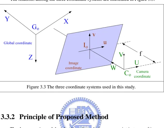
3.3.1 Coordinate Systems

The three coordinate systems used in this study are introduced at first. By these coordinate systems, it will be clear and convenient to describe a vehicle location. The definitions of the three coordinate systems are described in the following.

(1) The global coordinate system (GCS, denoted as X-Y-Z): In the global coordinate system, we assume that the two perpendicular lines of a corner on the ceiling are the X and Y axes, the vertical line is the Z axis, and the corner point is the origin Go of the global coordinate system.

(2) The camera coordinate system (CCS, denoted as U-V-W): In the camera coordinate system, we establish the U, V, and W axes. The U-V plane is parallel to the image plane, and the U axis is parallel to the X-Y plane of the global coordinate system. The origin Co is located at the camera lens center

and the W axis is aligned to be parallel with the camera optical axis.

(3) The image coordinate system (ICS, denoted as u-v): The image plane is located at W = f, where f is the focus length of the camera. The image plane of the image coordinate system is coincident with the u-v plane and the

origin Io is the image plane center.

The relations among the three coordinate systems are illustrated in Figure 3.3.

Figure 3.3 The three coordinate systems used in this study.

3.3.2 Principle of Proposed Method

The three equations of the edge lines through the corner point in terms of image coordinates (u, v) are described by u_p +b v_{i p}+ =c_i 0, where i=1, 2, 3. The desired vehicle location will be described by three position parameters Xc, Yc, and Zc and two

direction parameters ψ and θ, where Zc is the distance from the camera to the

ceiling and is assumed to be known, θ is the pan angle of a camera, and ψ is the tilt angle of the camera with respect to the global coordinate system. The five vehicle location parameters can be derived in terms of the four coefficients , , and

of the edge line equations in the corner image. Finally the vehicle location could be estimated after the coefficients of the edge line equations are computed.

1

b c₁ b₂

2 c

3.3.3 Location Estimation by Coefficients of Edge

Line Equations

In this section, we will derivate the relation between the global coordinates and the coefficients of the edge line equations in the image coordinate system. At first, we transform the global coordinates into the camera coordinates. The transformation consists of four steps.

Step 1 Translate the origin of the global system by

(

X Y Z_c, _c, _c

)

to the origin of the camera system in the following way:

(

)

1 0 0 0 0 1 0 0 , , 0 0 1 0 1 c c c c c c T X Y Z X Y Z ⎡ ⎤ ⎢ ⎥ ⎢ ⎥ = ⎢ ⎥ ⎢_{− − −} ⎥ ⎢ ⎥ ⎣ ⎦ . (3.1)

Step 2 Rotate the X −Y plane about the

Z

axis through the pan angle ψ in the following way such that the X −Y plane is parallel to the U V− plane:

( )

cos sin 0 0 sin cos 0 0 0 0 1 0 0 0 z R ψ ψ ψ ψ ψ − ⎡ ⎤ ⎢ ⎥ ⎢ ⎥ = ⎢ ⎥ ⎢ ⎥ ⎣ ⎦ 0 1 . (3.2)

Step 3 Rotate the Y−Z plane about the X axis through the tilt angle θ in the following way such that the X −Y plane is parallel to the U V− plane:

( )

1 0 0 0 0 cos sin 0 0 sin cos 0 0 0 0 1 x R θ θ θ θ θ ⎡ ⎤ ⎢ ₋ ⎥ ⎢ ⎥ = ⎢ ⎥ ⎢ ⎥ ⎣ ⎦ . (3.3)

Step 4 Reverse the

Z

axis in the following way such that the positive direction of the

Z

axis is identical to the negative direction of the W axis

1 0 0 0 0 1 0 0 0 0 1 0 0 0 0 1 z F ⎡ ⎤ ⎢ ⎥ ⎢ ⎥ = ⎢ − ⎥ ⎢ ⎥ ⎣ ⎦ . (3.4)

Now, if we have a point P with global coordinates ( ,x y z, ) and camera coordinates , the transformation in the two coordinate systems can be described in short as:

( , , )u v w

(

) ( ) ( )

( , , ,1)u v w =( , , ,1)x y z ⋅T X Y Z_c, _c, _c ⋅R_z ψ ⋅R_x θ ⋅F_z =( , , ,1)x y z T_r (3.5) where

(

) ( ) ( )

0 0 0 , ,

cos sin cos sin sin 0 sin cos cos cos sin 0 0 sin cos 1 r c c c z x z T T X Y Z R R F x y z ψ θ ψ ψ θ ψ θ ψ ψ θ ψ θ θ θ = ⋅ ⋅ ⋅ − − ⎡ ⎤ ⎢ ⎥ ⎢ ⎥ = ⎢ − ⎥ ⎢ ⎥ ⎢ ⎥ ⎣ ⎦ 0 (3.6) with 0 ccos csin x = −X ψ −Y ψ ;

(

)

0 csin ccos cos csin

y = X ψ−Y ψ θ−Z θ ;

(

)

0 csin csin sin ccos

z = X ψ−Y ψ θ+Z θ .

(3.7)

If P is on the X axis with global coordinates ( , , the camera coordinates

0, 0)

x

( ,u v w can be rewritten as: _{x x}, _x)

0 0

( , , , 1) ( , 0, 0, 1)

( cos , sin cos , sin sin ,1).

x x x r u v w x T x ψ x x ψ θ y x ψ θ z = ⋅ = + − + − + 0 (3.8) Let be the image coordinates of the projection of , then we have the following two equations to describe u

(u vp, p) P

x p x f u u w ⋅ = ; (3.9) x p x f v v w ⋅ = , (3.10) where f is the camera focus length.

Substituting the values of u and _x v , we may rewrite Formulas (3.9) and (3.10) _x

above for u and _x v as Equations 3.11 and 3.12 below: _x 0 0 ( cos ) sin sin p f x x u z ψ ψ θ ⋅ + = − + ; (3.11) 0 0 ( sin cos ) sin sin p f x y v z ψ θ ψ θ ⋅ − + = − + . (3.12)

Eliminating the variable x, we can get the equation for the projection of the

X-axis in the image plane as Equation 3.13 below:

0 0 0 0

0 0

( cos sin sin ) ( cos sin cos ) sin sin sin cos

p p v z x f y x u y z ψ ψ θ ψ ψ θ ψ θ ψ θ ⋅ − − + ⋅ + = − + . (3.13)

After substituting Equation 3.13 into u_p+b v_{1 p}+ =c₁ 0 and substituting Equation 3.7 for x , ₀ y , and ₀ , we obtain the coefficients and as described by Equations 3.14 and 3.15 below:

0

z b₁ c₁

1

sin cos cos sin c c c Y Z b Z θ ψ θ ψ − = − ; (3.14) 1

( cos cos sin sin c c c f Y Z c Z ) θ ψ θ ψ ⋅ − − = − . (3.15)

Similarly, the coefficients of the edge line equation up+b v₂ p+c₂ =0 for the

projection of the Y axis in the image plane can be derived to be as follows:

2

sin sin cos cos c c c X Z b Z θ ψ θ ψ − − = ; (3.16)

2

( cos sin sin cos c c c f X Z c Z ) θ ψ θ ψ ⋅ − = . (3.17) The next step is to determine the variables of directions, ψ and θ. First, we use Equations 3.14 and 3.15 to derive the variable ψ . Equations 3.14 and 3.15 can be transformed into Equations 3.18 and 3.19, respectively, described below:

1

( sin cos cos ) sin

c c

Z −b ψ + ψ θ =Y θ

c

; (3.18)

1

( sin cos cos ) cos

c

Z −c ψ + f ψ θ = −fY θ .

(3.19) By eliminating Z and _c Y_c from Equations 3.18 and 3.19, tanψ can be described as Equation 3.20 below:

1 1 tan cos sin f fb c ψ θ θ = + . (3.20)

Similarly, Equations 3.16 and 3.17 can be transformed into Equations 3.21 and 3.22, respectively, described below:

2

( cos sin cos ) sin

c

Z b ψ + ψ θ = −X_c θ

c

; (3.21)

2

( cos sin sin ) cos

c

Z c ψ + f ψ θ = fX θ.

(3.22) By eliminating Z and _c X from Equation 3.21 and 3.22, tan_c ψ can be rewritten as Equation 3.23 below shows:

2cos 2sin

tan fb c

f

θ θ

ψ = − − . _(3.23)

We can use Equations 3.20 and 3.23 to get tanθ as follows:

1 2 1 2 ( ) tan f b b c c θ =− + + . (3.24)

Thereafter, we can substitute the value θ into Equation 3.23 to obtain the value ψ . Finally, the values of θ, ψ , and Z are all known, and can be substituted into _c

3.4 Image Processing for Vehicle

Location Estimation

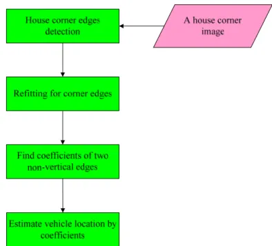
In order to conduct vehicle location estimation by house corner edges automatically, we need a series of image processing and numerical analyses to find the coefficients of the edge line equations in an image. A flowchart of the image processing and numerical analysis process is shown in Figure 3.4.

The main technique is to use the Hough transform to detect lines in an image. The process to find the house corner edges of an image captured from the PTZ camera is described in Section 3.4.1. After we find the house corner edges, the next step is to find the coefficients of the house corner edges. In order to improve the accuracy of the coefficients of the edge line equations, we use a constrained line refitting technique to refit the extracted lines into new ones. The constrained condition is that each edge line should go through the house corner point. Finally, since it is sufficient to estimate a vehicle location by only two non-vertical corner edges, we keep the necessary edges from the result of the Hough transform. Then the coefficients of the two non-vertical corner edges are computed. By the coefficients, the vehicle location can be estimated. In Section 3.4.2, we will discuss the proposed constrained line refitting technique and the restrictions for keeping two non-vertical edges.

Figure 3.4 Flowchart of vehicle location estimation.

3.4.1 Detection of House Corner Edges

In order to detect the edges of a house corner in an acquired image, we apply several image processing techniques to find out the edges. A flowchart is illustrated in Figure 3.5.

A house corner image captured by a PTZ camera may contain not only house corner edges but also a lot of other components. But we only need the house corner edges. The Hough transform is a powerful technique to detect straight lines in an image. In the Hough transform, each line is represented in the form of Equation 3.25 below:

cos sin

r=x α+y α (3.25) where x and y are the image coordinates of the line points, α is the direction of the normal of the line, and γ is the distance of the line to the origin of the image coordinate system. Each point in the image coordinate system is transformed into a curve with α and γ as the coordinates. All the curves corresponding to a set of

image points lying on a straight line will intersect at a point. Because the Hough transform is useful to detect straight lines, we use the technique to detect house corner edges in this study.

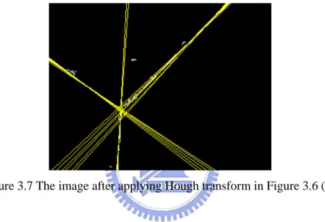
Before applying the Hough transform, we should find out the edges in an image. The Canny edge detection can help us to detect edges by an appropriate threshold. Figure 3.6 (a) is a house corner images and Figure 3.6 (b) is the result image after the Canny edge detection was applied respectively. Apparently the result shows the edge lines of the house corner clearly. However, it still contains other unconcerned edges.

(a) (b) Figure 3.6 (a) The color corner images. (b) The Canny result images of (a).

Because the house corner edges always extend to the boundary from the house corner point in an image, we can apply the Hough transform by a proper threshold, meaning that lines in an image must be long enough, to be regarded as house corner edges. Each line detected by the Hough transform is represented by the two parameters α and γ. Figure 3.7 shows the house corner edge lines after the Hough transform. Then we can obtain a set of house corner edge datarepresented by α and

γ. An algorithm including the above details is described in the following.

Figure 3.7 The image after applying Hough transform in Figure 3.6 (b).

Algorithm 3.1. House corner edges detection.

Input: A house corner image Icorner.

Output: A set of house corner edge data Ecorner.

Steps:

Step 1. Convert the image Icorner into a gray-level image Igray.

Step 2. Apply the Canny edge detection by the threshold Thcanny on Igray to obtain

a set of edges Ecorner in Igray.

Step 3. Apply the Hough transform by the threshold Thhough; reserve each detected

line which is longer than Thhough; and represent it by the parameters α

Step 4. Take the final results of house corner edges represented by α and γ as the desired set Ecorner.

More experimental results of corner edge detection shown in Figure 3.8 and Figure 3.9.

(a)

(b) (c) Figure 3.8 An experimental result of a different house corner. (a) Another corner image. (b)

The result of applying Canny edge detection of (a). The result of applying Hough transform of (b).

(a)

(b) (c) Figure 3.9 One more experimental result of another different house corner. (a) Another

corner image. (b) The result of applying Canny edge detection of (a). The result of applying Hough transform of (b).

3.4.2 Constrained Line Refitting and Determination

of Non-vertical House Corner Edges

Because the accuracy of vehicle location estimation depends on the precision of the coefficients of edge line equations, we use a constrained line refitting technique to reconstruct the house corner edge lines in an image. This process can improve the

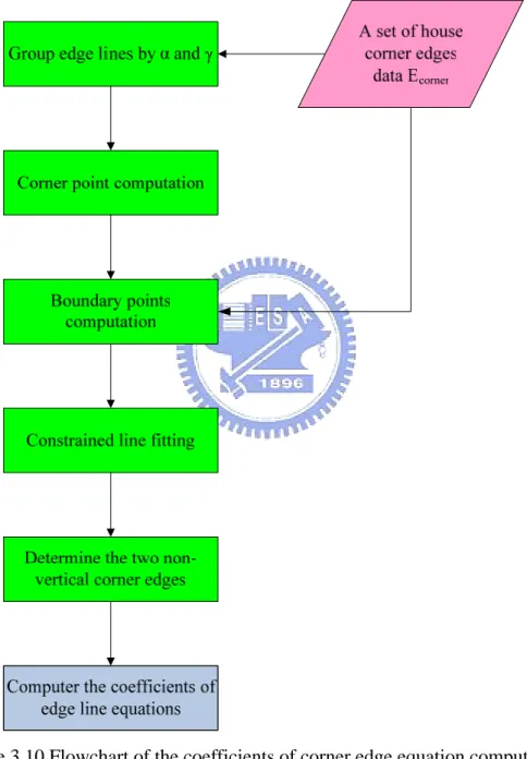
precision of house corner edge lines detected in an image. Moreover, in this study, two non-vertical corner edges are sufficient to estimate the vehicle location, so we have to find out them in the three edges of each corner image. The process for constrained line fitting and determination of non-vertical house corner edges is shown in Figure 3.10.

Figure 3.10 Flowchart of the coefficients of corner edge equation computation.

After the Canny edge detection and Hough transform are applied, corner edges are found in a house corner image. However, a found house corner edge may not

represent exactly a line in the image. In normal cases, after applying the Hough transform to a house corner image, more than three corner edge lines are detected. Thus, to group together lines with each group representing an edge line is useful for later processing.

We utilize the features of the House transform results, namely, the parameters α and γ of each detected line. We use these two parameters to group corner edge lines. If the parameter valuesα and γ of two lines are closer enough, then they are taken into the same group. Lines in an identical group mean that they represent the same house corner edge actually. An example is shown in Figure 3.11. The red lines come from a corner edge, and the blue line is another corner edge, and the green lines come for the third corner edge.

Figure 3.11 Illustration of a set of lines representing an identical house corner edge.

Now, we compute the intersections of all the detected lines, collect their image coordinates, and compute the average image coordinates as a new house corner point. At first, we transform lines described in terms of coordinates α and γ into ones described in terms of image coordinates. We represent each line as follows:

0 u bv c+ + = , (3.26) where 1 tan b α = ; (3.27) sin c γ α = . _(3.28)

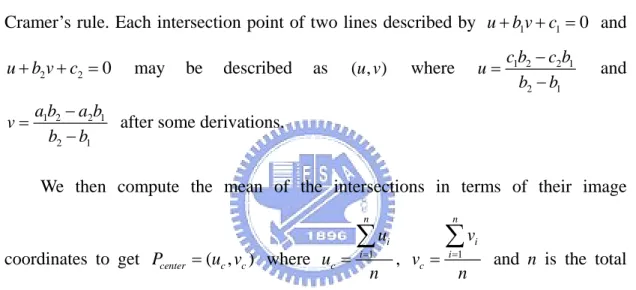
Then, the intersections of the lines in different groups can be computed by Cramer’s rule. Each intersection point of two lines described by and

may be described as where

1 1 0 u+b v+ =c 2 2 0 u b v c+ + = ( , )u v 1 2 2 1 2 1 c b c b u b b − = − and 1 2 2 1 2 1 a b a b v b b − =

− after some derivations.

We then compute the mean of the intersections in terms of their image

coordinates to get Pcenter =( ,uc vc) where

1 n i i c u u n = =

∑

, 1 n i i c v v n =

=

∑

and n is the total number of intersections. We take this point Pcenter as a final house corner point.

An example of the house corner point so found is shown in Figure 3.12. The new house corner point is then used to refit house corner edges later.

After we separate the three groups of house corner edges, we can take the pixels in the same group as the points of an edge line. Let the line points to be refitted are denoted by S =

{

(

u_i, v_i

)

,i=1, 2, ..., n

}

. An example of the set is shown in Figure 3.13. Let the refitting line L be represented as follows:

' '

u b v c+ + = 0 . (3.29)

Figure 3.13 The different color points represent the different edge respectively.

By the least-square-error fitting criterion, the line L satisfies that the sum of the squares of all the distances from the points in S to L is minimum and that the parameter b’ satisfies the following formula:

' ' b = −V c U, (3.30) where 1 n i i u U n = =

∑

; (3.31)

1 n i i v V n = =

∑

, (3.32)

with n being the number of elements in S.

We also constrain the line L to go through the house corner point Pcenter. Thus, we

can substitute the Pcenter into Equation 3.29 and describe c’ as follows:

' ( _c ' _c

c = − u +b v ) . (3.33) By Equations 3.30 and 3.33, we can obtain b' as follows:

' c c U u b V v − = − − . (3.34) ' c c c c U u c v V v − = − − u (3.35)

Therefore, we can represent each refitting line L by b’ and c’ described above. After such constrained line refitting is conducted, the precisions of the house corner edge lines are improved.

Finally, only two house corner edge lines are necessary in this study, and the unnecessary corner edge is the vertical line. Discarding of the vertical house corner edge can be accomplished by judging the slopes of the three refitted corner edge lines. An example is shown in Figure 3.14, and the color lines are non-vertical corner edge lines. By the two corner edge lines, the necessary coefficients are obtained. A detailed algorithm is described in the following

Figure 3.14 Refitting of two non-vertical corner edges.

Algorithm 3.2. Constrained line refitting and determination of non-vertical lines.

Input: A set of house corner edges described in terms of α andγ.

Output: the coefficients of non-vertical house corner edges. Steps:

Step 1. Group together lines whose α and γ are closer enough.

Step 2. Transform lines described in terms of coordinates α and γ into ones described in terms of image coordinates by Equation 3.26.

Step 3. Compute the intersections of the lines in different groups by Cramer’s rule.

Step 4. Compute the mean of the intersections in terms of image coordinates and denote the result as Pcenter.

Step 5. Collect edge line points in the same group into S.

Step 6. Refit line L by Equations 3.33 and 3.34 using the data of S and Pcenter.

Step 7. Determine the two non-vertical edges by the slopes of the three refitting edge line equations, with the slope of the vertical edge being taken to approach infinity.

More experimental results of constrained line refitting are shown in Figure 3.15 and Figure 3.16.

(a) (b)

(c) (d) Figure 3.15 An experimental result of a different house corner. (a) The sets of lines represent

an identical house corner edge. (b) The house corner center. (c) The edge points (d) Refitting of two non-vertical corner edges

(a) (b)

(c) (d) Figure 3.16 One more experimental result of another different house corner. (a) The sets of

lines represent an identical house corner edge. (b) The house corner center. (c) The edge points (d) Refitting of two non-vertical corner edges

Chapter 4

Obstacle Avoidance by Goal-Directed

Minimum-Path Following

4.1 Overview of Obstacle Avoidance

An obstacle appearing on navigation path suddenly is an ordinary situation in vehicle navigation. Many methods for obstacle avoidance have been proposed recently. Ku and Tsai [11] proposed a quadratic classifier for obstacle avoidance. Chen and Tsai [12] proposed a fuzzy guidance technique for the same purpose. However, most methods are specific in their applications. A general solution for obstacle avoidance is difficult. In order to avoid an obstacle in navigation, an obstacle avoidance method is necessary for our vehicle system. Because usually the navigation path is created in advance, the vehicle must avoid obstacles in real time. Therefore, detecting obstacles quickly is necessary to react to the situation.

The first step of obstacle avoidance is obstacle detection. The obstacle detection method used in this study is described in Section 4.2. If an obstacle is detected on the navigation path, a new path should be computed to avoid the obstacle. And the goal of the new path is toward the next node of the navigation path. The proposed process for this purpose is described in Section 4.3. The process of obstacle avoidance is illustrated in Figure 4.1.

In order to achieve the task, we need to know obstacle distributions in real space. Thus we define some coordinate systems and a direction angle of the vehicle in this

study at first. The coordinate systems are defined in Section 4.1.1 and the direction angle of the vehicle is defined in Section 4.1.2. By using the direction angle, transformations between these coordinate systems is possible. We utilize the transformation functions to obtain obstacle distributions in real space. The transformation function is described in Section 4.1.3.

Find floor area Start obstacle avoidance

Image I

Minimum-path computaion

Drive the vehicle by new path

Obstacle exists No

Yes Find obstacle distribution

Navigation is impeded by obstacle No

Yes

4.1.1 Coordinate Systems

In this study, the following two coordinate systems are used to describe the vehicle location and the navigation environment. These coordinate systems are illustrated in Figure 4.2 and defined in the following.

(a)

(b)

Figure 4.2 Two coordinate systems in this study. (a) The vehicle coordinate system. (b) The global coordinate system.

(1) The vehicle coordinate system (VCS, denoted as Vx-Vy): The origin Vo of the

vehicle coordinate system is placed at the middle point of the line segment which connects the two contact points of the two wheels with the ground. The Vx and Vy

Vy-axis is perpendicular to the Vx-axis.

(2) The world coordinate system (WCS, denoted as x-y): The origin Go of the world

coordinate system is located at a certain fixed position and it is the starting position of each navigation session in this study. The x-axis and the y-axis are defined to lie to on the ground and perpendicular to each other.

4.1.2 Direction Angle of Vehicle

We need to know the state of the vehicle heading, so we define the direction angle of the vehicle in the world coordinate system. The angle, denoted as ω, represents the rotation degree of the vehicle in the world coordinate system and plays an important role in coordinate transformation.

ω is the angle between the positive direction of the x-axis and the front of the vehicle. The direction angle ω is set to be zero at the beginning of navigation. The range of ω is between 0 and π if ω is in the first and second quadrants, as illustrated in Figure 4.3(a). It is between 0 and −π if ω is in the third and forth quadrants, as illustrated in Figure 4.3(b).

(a) (b) Figure 4.3 Definition of the direction angle (a) ω is positive. (b) ω is negative.

4.1.3 Coordinate Transformation

The transformation functions between the vehicle coordinate system and the world coordinate system using the direction angle is shown in Equation (4.1) and Equation (4.2) below, where xp and yp are the coordinates of the vehicle in the world

coordinate system. V sin_x V cos_{y p} x= ω− ω+x (4.1) V cos_x V sin_{y p} y= ω+ ω+y (4.2) The coordinate transformation between the vehicle coordinate system and the world coordinate system is illustrated in Figure 4.4.

Figure 4.4 The coordinate transformation between the vehicle coordinate system and vehicle coordinate system.

4.2 Obstacle Detection Process

Overall, before the obstacle avoidance process is started, a process to detect obstacles is applied first. In this study, we observe the floor continuously to obtain the floor area all the time. Finding the floor area is important and convenient for detection

of obstacles on the navigation path. The process to find an obstacle is described in Section 4.2.1. As long as we obtain the floor area, the floor in the image can be filtered out. Therefore, we can deal with a new image without the floor area. We define a warning area for obstacle alert at first. Once we detect anything in the area, it means that something extraordinary is on the floor. The process for determination of obstacle existence is described in Section 4.2.2. A flowchart of the obstacle detection process is illustrated in Figure 4.5.

4.2.1 Finding Floor Area

In order to find an obstacle on the floor, the first thing is to find the floor area in that image. One reasonable assumption is that there is no obstacle on the uniform floor in the initial image captured by the camera. Under this assumption, we can apply a region growing algorithm by an appropriate seed to find the floor area in the initial state. After finding the floor, we can retrieve the color feature of the floor and denote it as Cfloor. The color feature here is computed in terms of the R, G, and B color values.

The definition is 1 1 1 ( , , n n n i i i i i floor ) i R G B C n n n = = = =

∑ ∑ ∑

where Ri, Gi, BBi are the R, G, and B values of a pixel Pi in the image, and n is the

number of the floor pixels.

The color feature of floor is useful in determination of obstacle existence and finding a collision-free path later. In the first cycle, we perform a region growing algorithm with the initial color feature Cfloor as a seed to find the floor area and record

the new color feature of the floor area as Cfloor'. At the end of the process, we update

Cfloor to be Cfloor’ for thenext cycle. So in each cycle, we use the color feature of the

floor of the last navigation cycle to find the floor area of the current navigation cycle. A floor area found by this method is shown in Figure 4.6. The algorithm is described in detail as follows.

Algorithm 4.1 Finding floor area.

Input: A color image I.

Output: The floor area AREAfloor and the color feature Cfloor of the floor area.