利用位能場做部分表面之三維點雲車體形狀辨識

(1)

國

立

交

通

大

學

資訊學院資訊學程

碩

士

論

文

利用位能場做部分表面之三維點雲車體形狀辨識

Shape Matching of Partial 3D Point Cloud of a Vehicle Using

Artificial Potential Fields

研究生：李閏秋

指導教授：莊仁輝教授

(2)

利用位能場做部分表面之三維點雲車體形狀辨識

Shape Matching of Partial 3D Point Cloud of a Vehicle Using Artificial

Potential Fields

研究生：李閏秋 Student：Jun-Chiu Li

指導教授：莊仁輝 Advisor：Jen-Hui Chuang

國立交通大學

資訊學院資訊學程

碩士論文

A Thesis

Submitted to College of Computer Science National Chiao Tung University in partial Fulfillment of the Requirements

for the Degree of Master of Science

in

Computer Science January 2013

Hsinchu, Taiwan, Republic of China

(3)

i

利用位能場做部分表面之三維點雲車體形狀辨識

研究生：李閏秋

指導教授: 莊仁輝

國立交通大學資訊學院資訊學程碩士班

摘要

本論文之研究主要是利用位能場模型來做為三維汽車車體的形狀比對與辨識，此模型的做法是先將待測物縮小置於模型內部，再藉由待測物與模型彼此之間的推斥力與力矩作用位置調整及方向旋轉，再搭配放大及碰撞測試限制待測物必需在模型內，若兩者為相似的形狀，則待測物可放至最大，可得到待測物在模型中最大的佔有率，此時即可推估待測物是屬該模型，而達到辨識的效果。然而，由於通常所取得之汽車待測物並非完整的三維物體，因此雖然經過力的推斥計算仍無法達到最正確的位置，也可能無法達到理想的佔有率。所以本論文除了將此人工力場模型實現於真實汽車的車型辨識，也將最小投影矩形及分析待測物之點雲高度的觀念導入，使得辨識時將待測物調整至與 x-y-z 平行的位置，可使佔有率得到改善，而提升辨識可靠度。根據這個目標，本論文提出三種改善待測物位置的方法，分別是最小矩形作為待測物之正確位置之估計，點雲高度數量分析找出引擎蓋及車頂，使車體處於與模型平行的位置，而得到合理的車體辨識結果，實驗結果顯示本論文的方法可以提升辨識率而得到正確的車型識別。

(4)

ii

Shape Matching of Partial 3D Point Cloud of a Vehicle Using

Artificial Potential Fields

Student: Jun-Chiu Li

Advisor: Dr. Jen-Hui Chuang

Degree Program of Computer Science

National Chiao Tung University

ABSTRACT

In this thesis, the artificial potential field is used as the foundation for matching point cloud with 3D vehicular shapes. An initially small input object (point cloud) is placed inside shape models will experience repulsive force and torque arising from the potential field. A better match in shape between the shape model and the input object can be obtained if the input object translates and reorients itself to reduce the potential while growing in size. The shape model which allows the maximum growth of the input object corresponds to the best match and thus represents the shape of the input object. Since the point cloud does not cover the complete 3D object, the best match cannot be determined only by the potential model. Therefore, the research of this thesis also considers the minimum bounding boxes of projections of the point cloud and the distribution of objects points in the z-direction to improve the matching results. Based on the above concept, three methods are considered to refine the shape matching results via silhouette minimization, hood finding and roof finding. Experiment results show that the methods proposed in this thesis can indeed increase the rate of recognition of real vehicular shapes.

(5)

iii

AKNOWLEDGEMENTS

First and foremost, I would like to express my deepest gratitude to my advisor, Dr. Jen-Hui Chuang. Ever since I became Dr. Chuang’s student, I have learned so much from him academically. He spent a tremendous amount of time leading me in researching, academic findings, data collecting, and finally, finishing my thesis. He has also taught me a great deal in fields of patience, motivation, enthusiasm, and immense knowledge. I am also grateful for Drs. Chien-Chou Lin and Yong-Sheng Chen for spending time in reading and providing useful suggestions about this thesis.

Additionally, I would like to thank my fellow labmates in Intelligent System Lab for the stimulating discussions, and for all the fun we have had in the last some years.

Last but not the least; I would like to thank my colleagues and family for supporting me spiritually throughout my life. It is impossible for me to finish my education seamlessly without their support.

(6)

iv

LIST OF FIGURES

Figure 1-1 Object and model ... 1

Figure 2-1 A polygonal surface S in the 3D space. ... 4

Figure 2-3 (a) Example of template (b) Example of object (points) ... 7

Figure 2-4 The basic shape-matching procedure: (a) places a (size-reduced) input object inside a template object, (b) translates and (c) rotates the input object to reduce the potential, then (d) increase the size of the input object. ... 8

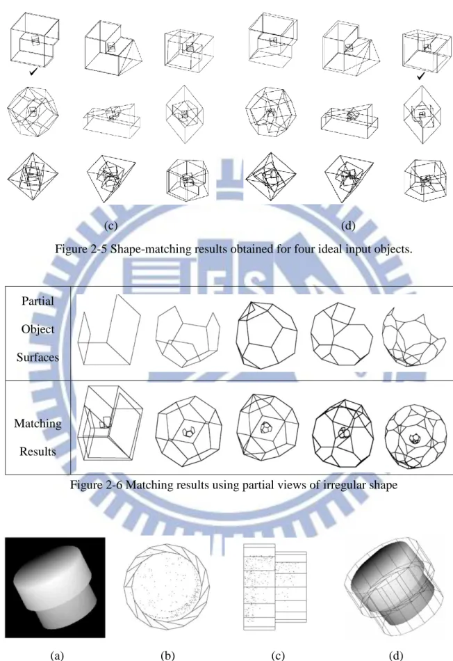
Figure 2-5 Shape-matching results obtained for four ideal input objects. ... 10

Figure 2-6 Matching results using partial views of irregular shape ... 10

Figure 2-7 Shape Matching results for real object (range data) ... 10

Figure 3-1 3D Object Recognition Flow ... 11

Figure 3-2 Contents of obj file ... 12

Figure 3-3 Matching results of ideal objects ... 14

Figure 3-4 Real vehicle objects (a) Object 1 (a sedan); (b) Object 2 (another sedan); ... 15

(c) Object 3 (an SUV)... 15

Figure 3-5 Shape matching results for Object 1 ... 16

Figure 4-1 Bounding box to be minimized for shape matching ... 20

Figure 4-2 Finding minimum bounding box area for the object shown in Figure 4-1 via rotation with respect to the z-axis ... 21

Figure 4-3 Finding minimum bounding box area for the object shown in Figure 4-1 via rotation with respect to the x-axis ... 22

Figure 4-4 Finding minimum bounding box area for the object shown in Figure 4-1 via rotation with respect to the y-axis ... 23

Figure 4-5 Object (front view) and z-value histogram of two different object orientations .... 25

Figure 4-6 Comparison of z-value histograms for four object orientations ... 25

Figure 4-7 Peak z-values of the object rotated with respect to the y-axis ... 26

Figure 4-8 (a) Object with a 24-degree rotation (b) The z-value histogram ... 26

Figure 4-9 Peak z-value of the object rotated with respect to the x-axis ... 27

Figure 4-10 (a) Object with a -4-degree rotation (b) The z-value histogram ... 27

Figure 4-11 (a) Object with a 5-degree rotation (b) The z-value histogram ... 28

Figure 4-12 local peak of z-value and maximum of zero counts versus different x rotation ... 29

Figure 5-1 Matching results for Object 1 by the procedure of SHR (original: blue, refinement: red) ... 31

(9)

vii

Figure 5-2 Matching results for Object 1 by the procedure of SRH (original: blue, refinement: red) ... 31 Figure 5-3 Matching results for Object 1 by the procedure of HRS (original: blue, refinement: red) ... 32

Figure 5-4 Matching results for Object 1 by the procedure of HSR (original: blue, refinement: red) ... 32

Figure 5-5 Matching results for Object 1 by the procedure of RSH (original: blue, refinement: red) ... 32 Figure 5-6 Matching results for Object 1 by the procedure of RHS (original: blue, refinement: red) ... 33

Figure 5-7 Matching results for Object 2 by the procedure of SHR (original: blue, refinement: red) ... 33

Figure 5-8 Matching results for Object 2 by the procedure of SRH (original: blue, refinement: red) ... 33

Figure 5-9 Matching results for Object 2 by the procedure of HRS (original: blue, refinement: red) ... 34 Figure 5-10 Matching results for Object 2 by the procedure of HSR (original: blue, refinement: red) ... 34 Figure 5-11 Matching results for Object 2 by the procedure of RSH (original: blue, refinement: red) ... 34 Figure 5-13 Matching results for Object 3 by the procedure of SHR (original: blue, refinement: red) ... 35 Figure 5-14 Matching results for Object 3 by the procedure of SRH (original: blue, refinement: red) ... 35 Figure 5-15 Matching results for Object 3 by the procedure of HRS (original: blue, refinement: red) ... 36 Figure 5-16 Matching results for Object 3 by the procedure of HSR (original: blue, refinement: red) ... 36 Figure 5-17 Matching results for Object 3 by the procedure of RSH (original: blue, refinement: red) ... 36 Figure 5-18 Matching results for Object 3 by the procedure of RHS (original: blue, refinement: red) ... 37 Figure 5-19 Test results of the three refinements without using the potential field model ... 38

(10)

viii

LIST OF TABLES

Table 3-1 Description of symbols in an obj file ... 13

Table 3-2 Comparison of the computation time for different implementations ... 14

Table 3-3 Summary of matching results for three real vehicle objects ... 19

Table 4-1 Summary of silhouette minimization ... 24

Table 4-2 Summary of hood finding ... 28

Table 4-3 Summary of roof finding ... 29

Table 5-1 The comparison of performance improvements for different sequences of refinement procedures... 31

(11)

1

Chapter 1. Introduction

1.1 Motivation

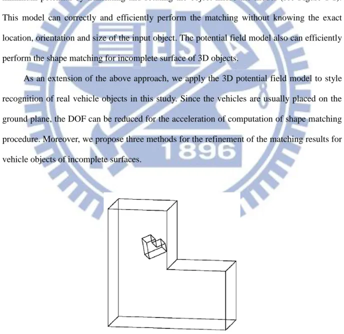
One of the major problems in computer vision is object recognition. Many existing algorithms simplify the problem by reducing it to a shape matching and recognition problem. Chuang et al. [1] propose a novel method using a potential field model for matching and recognition of 3D objects. This potential model computes total force and torque to find minimum potential by translating and rotating the object inside the model (see Figure 1-1). This model can correctly and efficiently perform the matching without knowing the exact location, orientation and size of the input object. The potential field model also can efficiently perform the shape matching for incomplete surface of 3D objects.

As an extension of the above approach, we apply the 3D potential field model to style recognition of real vehicle objects in this study. Since the vehicles are usually placed on the ground plane, the DOF can be reduced for the acceleration of computation of shape matching procedure. Moreover, we propose three methods for the refinement of the matching results for vehicle objects of incomplete surfaces.

(12)

2

1.2 Review of Related Works

3D object recognition is one of the challenging problems in computer vision. The recognition is more difficult than the 2D cases because of the higher degrees of freedoms. Most of 3D recognitions are extended from the 2D views. Several recognition systems extract features from 2D images and match them to corresponding features in a database of 3D models. The process is a procedure of verifying each candidates and finally ranking the verified candidates. In [3], some invariant features are extracted from triplet of surfaces and then constructed into an invariant feature indexing (IFI) of interpretation table. In the verification process, the extracted features are used to prune the candidates which are incorrect. A method based on the rotational symmetry is proposed in [4] to reduce the number of candidates. Further improvement is proposed in [5] based on a multi-view and multi-group approach. In the BONSAI system proposed in [6], a constrained search mechanism is used. The features extracted from the CAD model are represented by an interpretation tree (IT) and the search space is pruned by pose estimation.

Some approaches of recognition of 3D objects from 2D images use different image features. In [7], triangle pairs and quadrilateral pairs are used as features. In [8], edges of a 3D object are described by second-order equations and a transformation from a feature of a 3D object model to a 2D image feature is established. With such a transformation, proper alignment between a transformed 3D model and a possible image of the model can be obtained. In [9], the edges of a polyhedral 3D model are described by a weighted graph and the matching process is carried out using the Laplacian matrix. In [10], probabilistic indexing is used to determine whether there is a correspondence between projections of a 3D model and a 2D image. In [11], Fourier transform of the boundary description of a 3D model is first obtained, which is used in the matching through clustering.

(13)

3

representation and recognition of 3D objects using the finite element method. In [12], in order to define virtual forces which deform an object to fit a set of data points, springs are attached to pairs of corresponding object and data points. The shape matching is achieved by identifying the equilibrium displacement of the springs. In [13], a dynamic balloon model represented by using a triangular mesh is driven by an outward inflation force, while the vertices in the mesh are linked to neighboring vertices through springs to simulate the surface tension and to keep the shell smooth, until the mesh elements reach the object surface. The system includes an adaptive local triangle mesh subdivision scheme that results in an evenly distributed mesh. In [14], a 3D object is regarded as an isolated conductor. By assuming a piecewise constant charge density for each triangle of a triangular mesh, the segmentation is achieved by identifying surface concavities by tracing local charge density minima.

In this study, we use a novel way of using generalized potential model for 3D real vehicle shape matching. This method only needs partial surface information of the objects, in form of point cloud, without knowing the original location, orientation or size of the objects.

1.3 Thesis Organization

The remainder of this thesis is organized as follows. In Chapter 2, the 3D potential models and its application in shape recognition is reviewed. In chapter 3, an extension of the above approach is proposed for style recognition of real vehicle objects. Since the vehicles are placed on the ground plane, the less DOF are used to accelerate the computation of shape matching procedure. In chapter 4, three methods are considered to refine the matching results for vehicle of incomplete surfaces. Some experimental results are presented in chapter 5 to show the effectiveness and efficiency of the proposed approach. Finally, conclusions of this thesis and some future directions are given in Chapter 6.

(14)

4

Chapter 2. Reviews of Adopted Potential Models

2.1 A Review of the Generalized Potential Model

In Chuang [2], a potential-based approach for recognizing the shape of a two- dimensional (2D) region by identifying the best match from a selected group of shape templates is proposed. A better match in the shape between the template and the sample could be obtained if the template translates and reorients itself to reduce the potential while increasing in size. The shape sample with the largest final size corresponds to the best match and represents the shape of the given template. Afterward, Chuang et al. [1], utilize a 3D potential field model, called the generalized 3D potential model, which is extended from the 2D potential field model to assist the matching and recognition of 3D objects.

2.2 Equation of 3D Potential Modeling

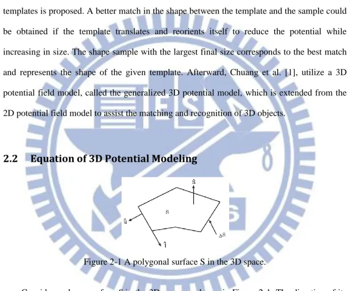
Figure 2-1 A polygonal surface S in the 3D space.

Consider a planar surface S in the 3D space as shown in Figure 2-1. The direction of its boundary, S, is determined with respect to its surface normal, 𝐧̂, by the right-hand rule,

𝐮

̂ × 𝐥̂ = 𝐧̂, where 𝐮̂ and 𝐥̂ are along the (outward) normal and tangential directions of S,

respectively. For the generalized potential function, the potential value at point r is defined as ∫ ， m  2. (2.1) Where R= | r - r |, for point r, r S and integer m is the order of the potential function.

(15)

5

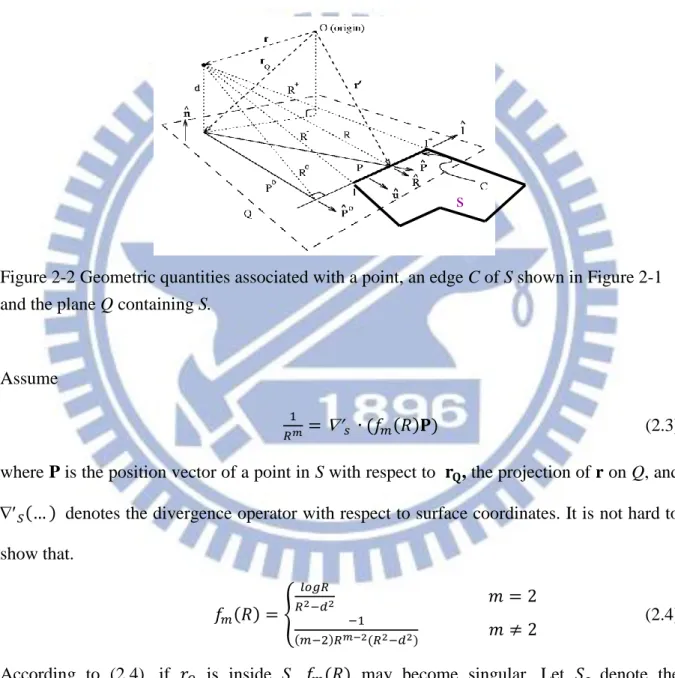
Related geometric quantities associated with an edge Ci of S in the plane containing S, Q, are shown in Figure 2-2 for r Ci. Without loss of generality, it is assumed that

d 𝐧̂ ( r-r ) > 0, (2.2)

which is equal to the distance from r to Q.

Figure 2-2 Geometric quantities associated with a point, an edge C of S shown in Figure 2-1 and the plane Q containing S.

Assume

 ) ) (2.3) where P is the position vector of a point in S with respect to , the projection of r on Q, and

 ) denotes the divergence operator with respect to surface coordinates. It is not hard to show that. ) { ) ₎

(2.4)

According to (2.4), if is inside S, ) may become singular. Let denote the

intersection of S and a small circular region on Q of radius and centered at , the potential

due to S can be evaluated as

(16)

6 ∫  [∫  ) )  ∫  ] (2.5) = ∑ ̂ ∫ )  ) where ( ) √  ( ) ) (2.6) ) { ) (2.7)

is the distance between r and Ci; is measured from the projection of r on Ci along the direction of 𝐥̂ ; and is the angular extent of  lying inside S as  0.

Since ) is a rational function for even m’s when m  2 and is rationalizable for odd m’s (see [15]), the line integrals can always be evaluated in closed form except for m = 2. For example, if  0, then we have

∫ ) ∫ ) [ ] (2.8)

The potential due to a polyhedron can then be obtained by calculating (2.5) for each polygonal face and then superposing the results. For example, if m=3, (2.5) can be expressed as

∫  ∑ [ ) )] (2.9)

where, for each Ci, the triple , and z are measured along 𝐥̂ , -𝐮̂ and 𝐧̂, respectively, with the origin located at the projection of r on Ci. It is not hard to show that (for simplicity, subscript i is omitted here)

)

√ (2.10)

For brevity, only the generalized potential of the third order, m = 3, will be considered in the rest of this thesis.

(17)

7

( ) ) (2.11)

The evaluation of the repulsion between templates and objects involves the calculation of the repulsion between pairs of surface and point with each pair having a surface from the template and a point from object. Usually, as shown in Figure 2-3, it is desirable that the sampling points are located uniformly on surfaces of the object.

(a) (b)

Figure 2-3 (a) Example of template (b) Example of object (points)

2.3 3D Shape Matching Procedure Using Potential Model

Based on the principle in Section 2.2, we give a brief figure to describe the shape matching-process. The following operations are performed with an input object being placed inside a template object (see Figure 2-4).

Step 1: Potential minimization through translations

(a) Computes the total force between the template and the input object to determine the minimum potential position of the latter along the above force direction.

(b) Repeats (a) until the results of two consecutive executions of (a) is negligible, in terms, the minimal potential position is determined.

Step 2: Potential minimization through rotations

(a) In order to compute the total repulsive torque between the template object and the input object, the centroid of the input object must be chosen as the rotation center. By rotating the object along the axis with the above torque direction, the angular

(18)

8

position of the minimal potential for the input object could then be found.

(b) Repeats (a) until an execution of the angular position of the input object could be found.

Step 3: Scaling

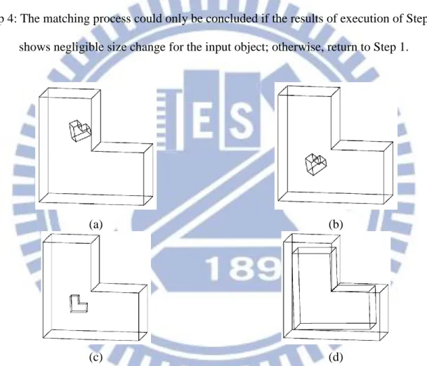
In order to locate the maximum size of the input object, the centroid of the input object is fixed in space, and the object remains inside the template with certain constraints. Step 4: The matching process could only be concluded if the results of execution of Step 3

shows negligible size change for the input object; otherwise, return to Step 1.

(a) (b)

(c) (d)

Figure 2-4 The basic shape-matching procedure: (a) places a (size-reduced) input object inside a template object, (b) translates and (c) rotates the input object to reduce the potential, then (d)

(19)

9

2.4 A Review of Shape Matching of [1]

Figure 2-5 shows some ideal shape matching results given in [1]. There are four shapes (a, b, c, d) in this particular matching examples. The pictures which have symbol “√” are the best matching results. One can see that all of these shapes result in good matching results. Figure 2-6 shows partial object surfaces of some shape templates and the corresponding shape-matching results. For all of these shapes, reasonable matching results can also be achieved. Figure 2-7 shows successful shape matching for point cloud of an object with cylindrical symmetry in shape. In all these situations, objects can all be matched and recognized efficiently using the analytically derived expressions associated with the potential function. In this thesis, we propose to apply the same potential model to real vehicle objects for style matching and recognition, with simplification in the implementation for the ground plane constraint for the location of the vehicles.

(20)

10

(c) (d)

Figure 2-5 Shape-matching results obtained for four ideal input objects.

Partial Object Surfaces

Matching Results

Figure 2-6 Matching results using partial views of irregular shape

(a) (b) (c) (d)

(21)

11

Chapter 3. Potential-Based Shape Matching

System

In this chapter, we will first introduce the flow in Section 3.1 which is similar to that described in Section 2.3. The detailed object data format is described in Section 3.2. Finally, the test results for some real vehicles objects are shown in Section 3.3.

3.1 Implementation Flow

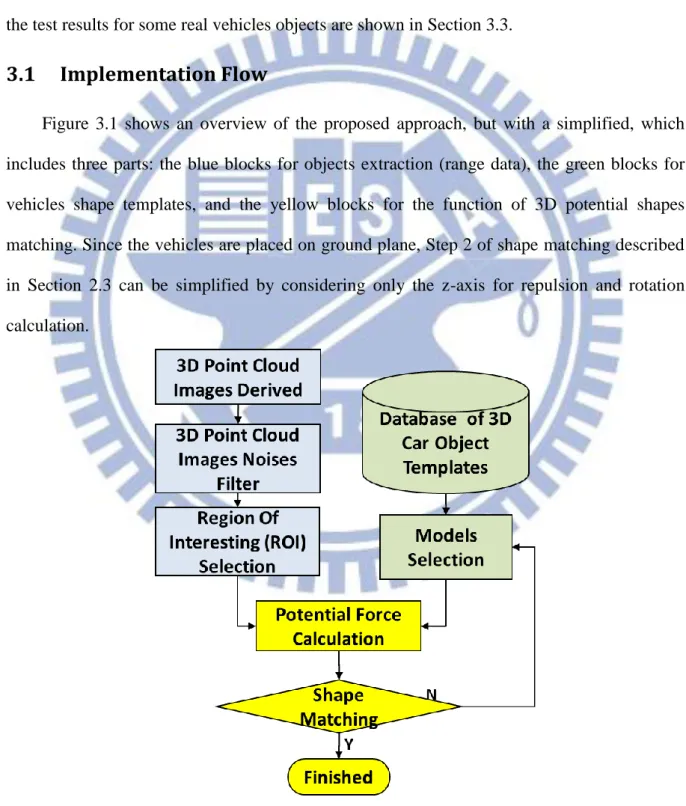
Figure 3.1 shows an overview of the proposed approach, but with a simplified, which includes three parts: the blue blocks for objects extraction (range data), the green blocks for vehicles shape templates, and the yellow blocks for the function of 3D potential shapes matching. Since the vehicles are placed on ground plane, Step 2 of shape matching described in Section 2.3 can be simplified by considering only the z-axis for repulsion and rotation calculation.

(22)

12

3.2 Range Data Format of Objects

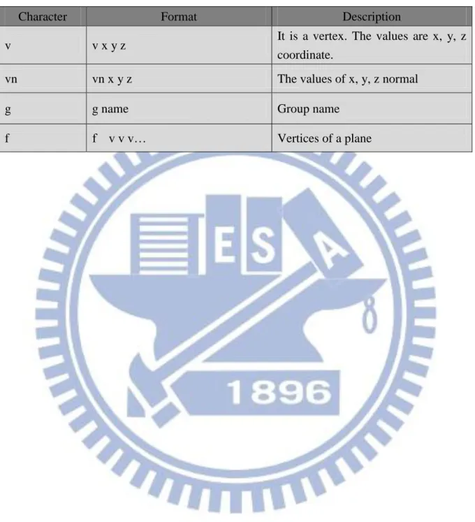
In this study, data file of *.obj format is chosen since it is the standard 3D object file format which is developed by Wavefront Technologies Company. The contents of obj files include coordinates of vertex and normal which are used to define the construction of polygons to form a 3D object. A text editor can be used to create, modify, and maintain the obj files easily. An example of *obj format is shown in Figure 3-2 with more detailed description of symbols used in the file given in Table 3-1.

Figure 3-2 Contents of obj file # this is a comment

# List of Vertices, with (x,y,z) coordinates v 0.123 0.234 0.345

v .. ...

# Normals in (x,y,z) form vn 0.707 0.000 0.707 vn ...

... #Group g group_name

# Face Definitions (see below) f 1 2 3

f 3/1 4/2 5/3 f 6/4/1 3/5/3 7/6/5 f ...

(23)

13

Table 3-1 Description of symbols in an obj file

Character Format Description

v v x y z It is a vertex. The values are x, y, z coordinate.

vn vn x y z The values of x, y, z normal

g g name Group name

(24)

14

3.3 Shape Matching Results of Real Vehicle Object

In Section 3.3.1, we use ideal objects (templates) for matching test. The two implementations of shape matching basically give the same results, which adjust the object orientation shape by (i) step 2 in Section 2.3 and (ii) simplification of (i) by considering only the z-axis. In Section 3.3.2, we use real vehicles as objects and assume that vehicles are placed on ground plane that the rotation along the x and y axes can be neglected.

3.3.1 Ideal Object Matching

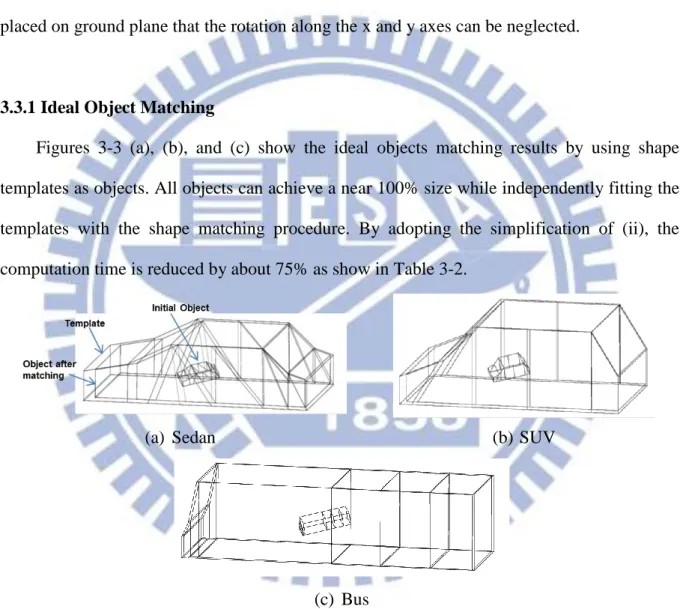
Figures 3-3 (a), (b), and (c) show the ideal objects matching results by using shape templates as objects. All objects can achieve a near 100% size while independently fitting the templates with the shape matching procedure. By adopting the simplification of (ii), the computation time is reduced by about 75% as show in Table 3-2.

(a) Sedan (b) SUV

(c) Bus

Figure 3-3 Matching results of ideal objects

Table 3-2 Comparison of the computation time for different implementations (Unit: sec.) Sedan SUV Bus

(i) 20 12 9

(25)

15

3.3.2 Real Vehicles Object Matching

In this Section, three templates which are shown in Section 3.3.1 are used for the shape matching of three real vehicle objects (see Figure 3-4 (a), (b), and (c)). The matching results of Object 1, Object 2, and Object 3 using three templates shown in Figure 3.3 are shown in Figure 3-5, Figure 3-6, and Figure 3-7, respectively.

Figure 3-4 Real vehicle objects (a) Object 1 (a sedan); (b) Object 2 (another sedan); (c) Object 3 (an SUV)

(26)

16

(a) Side view of Object 1 and sedan (b) oblique view of Object 1 and sedan

(c) Side view of Object 1 and SUV (d) oblique view of Object 1 and SUV

(e) Side view of Object 1 and bus (f) oblique view of Object 1 and bus Figure 3-5 Shape matching results for Object 1

(27)

17

(28)

18

A summary of matching result is shown in Table 3-3. One can see that, the matching results are generals correct; however, the differences in occupational rate are not conspicuous between sedan and SUV. On the other hand, it is observed that the position of objects after

(29)

19

matching in Figure 3-5~7, can be optimized. The matching results can be more accurate by adjusting their positions/orientations. Based upon this observation, this thesis proposes some refinement schemes, as discussed next.

Occupation rate = [Object (Max.y) / Template (Max.y)] % (3.1)

Table 3-3 Summary of matching results for three real vehicle objects

Template Point cloud object

Sedan(35 faces) SUV(97 faces) Bus(26 faces) Occupational rate (%) Object 1(sedan) (538 vertices) 75.63 72.76 _47.45 Object 2 (sedan) ( 447 vertices) 70.86 68.65 _44.25 Object 3 (SUV) ( 268 vertices) 68.56 72.60 _40.98

(30)

20

Chapter 4. Refinements of Shape Matching

Results

In this chapter, we describe three refinements of adjusting object position/orientation for better shape matching which include (i) refinements via bounding box minimization, (ii) refinements via hood finding, and (iii) refinements via roof finding.

4.1 Refinement via Silhouette Minimization

4.1.1 The Idea

Since a vehicle may roughly have rectangular shape when viewed from some orthogonal directions, the silhouette of the vehicle in x-y, y-z and z-x planes may be minimized for 3D shape matching. The above idea can also be simplified by minimizing the area of the bounding box of such silhouettes (see Figure 4-1).

(31)

21

4.1.2 Implementation Details

Figure 4-2 (a) shows the values of bounding box area (x × y) for the object shown in

Figure 4-1 rotating with respect to the z-axis from -30 degrees to 30 degrees. When the object rotates 14 degrees, the minimum area can be achieved. Figure 4-2 (b) shows the projection of the object (points) on the x-y plane, i.e., the top view, after such a rotation. One can see that the major direction of the projection and the y-axis are nearly paralleled. The result looks reasonable and seems to be the best orientation for shape matching when the vehicle is viewed along the z-axis. Figures 4-2 (c) and (d) show the perspectives from the front and the side of the vehicles.

(a) Bounding box area (x × y) for object

rotating with respect to the z-axis

(b) Original (black) and rotated (red) object points (top view)

(c) Original (black) and rotated (red) object points (front view)

(d) Original (black) and rotated (red) object points (side view)

Figure 4-2 Finding minimum bounding box area for the object shown in Figure 4-1 via rotation with respect to the z-axis

(32)

22

Figure 4-3 (a) shows values of bounding box area (y × z) for the above object rotated

with respect to the x-axis from -30 degrees to 30 degrees. When the object rotates -1 degrees the minimum area can be achieved. Figure 4-3 (b) shows the object position after the -1 degree rotation. The bounding box of the vehicle on the x-y plane is not much different from that in Figure 4-2(b). Moreover, for its front view is shown in Figure 4-3 (c), the object still has a big tilt in its orientation. In other words, the refinement has little to achieve via the rotation with respect to the x-axis. Figure 4-3 (d) shows similar results.

(a) Bounding box area (y × z) via object

rotation with respect to the x-axis

(b) Original (red) and rotated (blue) object points (top view)

(c) Original (red) and rotated (blue) object points (front view)

(d) Original (red) and rotated (blue) object points (side view)

Figure 4-3 Finding minimum bounding box area for the object shown in Figure 4-1 via rotation with respect to the x-axis

(33)

23

Figure 4-4 (a) shows the values of bounding box area (x × z) for the above object

rotated with respect to the y-axis from -30 degrees to 30 degrees. When the object rotates -2 degrees the minimum area can be achieved. Figures 4-4(b), (c), and (d) show the object position after the -2-degree rotation. One can see that such refinement has little effect in shape matching, as in Figure 4-3.

(a) Bounding box area (y × z) via object

rotation with respect to the x-axis

(b) Original (blue) and rotated (green) object points (top view)

(c) Original (blue) and rotated (green) object points (front view)

(d) Original (blue) and rotated (green) object points (side view)

Figure 4-4 Finding minimum bounding box area for the object shown in Figure 4-1 via rotation with respect to the y-axis

(34)

24

Table 4-1 summarizes the above area minimization for rotations with respect to different axes of the 3D coordinate system. Since only the object bounding box area in the x-y plane can be significantly adjusted, via rotation with respect to the z-axis, such a rotation is regarded as the first refinement of the object configuration.

Table 4-1 Summary of silhouette minimization Projection plane Rotation Angle (degrees) Area Reduction

x-y 14 Significant

y-z -1 Minor

x-z -2 Minor

4.2 Refinement via Hood Finding

4.2.1 The Idea

It can get the most points at the height of the hood when the vehicle paralleled the ground. This refinement is called hood finding.

After the above refinement of object orientation for rotation axis used in section 4.1, additional refinement (hood finding for) using other axes can be evaluated by observing the

z-value histogram of the same object. For example, Figure 4-5 (a) shows that the object still

has a tilted orientation while Figure 4-5 (b) shows the z-value histogram of Figure 4-5 (a). On the other hand, Figure 4-5 (c) shows a better object configuration which has an orientation more parallel to the x-y plane with Figure 4-5 (d) showing its z-value histogram. In Figure 4-5 (d), a peak at z-value range [1.3m, 1.6m] is noticeable for a particular rotation angle with respect to the y-axis. Additional histograms for different object orientations around such an angle are shown in Figure 4-6 in which a high point can be found in each histogram. The object orientation in Figure 4-6 (b), which has the maximum peak value, is chosen as the final result.

(35)

25

(a) Original object (b) z-value histogram of original position

(c) Object rotated by 23 degrees (d) z-value histogram after a 23-degree rotation

Figure 4-5 Object (front view) and z-value histogram of two different object orientations

(a) z-value histogram after a 20-degree rotation (b) z-value histogram after a 21-degree rotation

(c) z-value histogram after a 22-degree rotation (d) z-value histogram after a 23-degree rotation

(36)

26

The object is shown in Figure 4-5 is used to implement the refinement considered in this subsection. Figure 4-7 shows peak z-values when the object is rotated with respect to the

y-axis from -30 degrees to 30 degrees. When the object rotates 24 degrees the maximum of

peak z-values can be achieved. Figure 4-8 shows the orientation and z-value histogram after this refinement. Figure 4-9 shows maximum of peak z-values when the object is rotated with respect to the x-axis from -30 degrees to 30 degrees. When the object rotates -4 degrees the maximum of peak z-values can be achieved. Figure 4-10 shows the orientation and z-value histogram after this refinement.

Figure 4-7 Peak z-values of the object rotated with respect to the y-axis

(a) (b)

(37)

27

Figure 4-9 Peak z-value of the object rotated with respect to the x-axis

(a) (b)

(38)

28

Table 4-2 summarizes the above hood finding results for rotations with respect to different axes of the 3D coordinate system. Since the object can only be significantly adjusted via rotation with respect to the y-axis, such a rotation is regarded as the second refinement of the object configuration.

Table 4-2 Summary of hood finding

Direction Rotation Angle (degrees) Object Adjustment

x-z 24 Significant

y-z -4 Minor

4.3 Refinement via Roof Finding

4.3.1 The Idea

Since the roofs of most vehicles are almost planar, we may also get local peak z-value at the roof of the vehicle if the roofs are almost planar. Consider such an orientation of a vehicle shown in Figure 4-11 (a), and its z-value histogram shown in Figure 4-11 (b) the statistic result show that there is no object point (zero value) above the roof. Therefore, the two conditions for finding the roof (z value) include:

a. There are enough zero counts of z-values at the end of the histogram. b. The first non-zero count of z-value in the histogram is a local peak.

(a) (b)

(39)

29

The refinement conditions (a) and (b) described in section 4.3.1 are used to implement the object refinement by rotation with respect to x-axis. Figure 4-12 shows the above local peak of z-value (red) and the corresponding zero counts (blue) for rotation angles ranging -30 degrees to 30 degrees. The maximum z-value of local peak and a satisfactory zero count are achieved when the object is rotated by 5 degrees. Figure 4-13 shows the object and its z-value histogram after the roof finding. It seems that the object is finally adjusted to align with the 3D coordinate system.

Figure 4-12 local peak of z-value and maximum of zero counts versus different x rotation

Table 4-3 summarizes the above roof finding results for object rotation with respect to

x-axis.

Table 4-3 Summary of roof finding

Direction Rotation Angle (degrees) Object Adjustment

(40)

30

Chapter 5. Experimental Results

In this chapter we will provide three experimental results. In Section 5.1, we will try different order of the three refinement sequences and give a comparison/suggestion. In Section 5.2, we will examine the effect of only applying three refinements (without using potential model) for shape matching. In Section 5.3, experimental results show that three different vehicles can be matched correctly with the proposed potential minimization and refinement procedures.

5.1 Comparison of Implementation Procedures

We have tried six different order of performing the refinement procedures discussed in chapter 4, which include:

a. SHR: Oder silhouette minimization, hood finding, and roof finding. b. SRH: Oder silhouette minimization, roof finding, and hood finding. c. HRS: Oder hood finding, roof finding, and silhouette minimization. d. HSR: Order hood finding, silhouette minimization, and roof finding. e. RSH: Order roof finding, silhouette minimization, and hood finding. f. RHS: Order roof finding, hood finding, and silhouette minimization.

The comparison of performance improvements for different sequences of refinement procedures are shown in Table 5-1. Figures 5-1~5-9 show the matching results of Object 1~3 for above sequences of refinement procedures which achieve approximately same improvements.

(41)

31

Table 5-1 The comparison of performance improvements for different sequences of refinement procedures Sequence Occupational rate Run time Object SHR SRH HRS HSR RSH RHS Object 1(Sedan) (538 vertices) 84.47% 121 s 83.81% 131 s 84.54% 127 s 84.11% 125 s 84.12% 114 s 85.7% 116 s Object 2 (Sedan) ( 447 vertices) 86.96% 103 s 87.67% 100 s 87.61% 99 s 88.33% 88 s 87.67% 87 s 87.13% 92 s Object 3 (SUV) ( 268 vertices) 93.25% 34 s 91.67% 37 s 92.92% 38 s 92.14% 35 s 92.95% 35 s 92.91% 37 s

(a) Front view (b) Side view

Figure 5-1 Matching results for Object 1 by the procedure of SHR (original: blue, refinement: red)

Figure 5-2 Matching results for Object 1 by the procedure of SRH (original: blue, refinement: red)

(42)

32

Figure 5-3 Matching results for Object 1 by the procedure of HRS (original: blue, refinement: red)

Figure 5-4 Matching results for Object 1 by the procedure of HSR (original: blue, refinement: red)

Figure 5-5 Matching results for Object 1 by the procedure of RSH (original: blue, refinement: red)

(43)

33

(c) Front view (d) Side view

Figure 5-6 Matching results for Object 1 by the procedure of RHS (original: blue, refinement: red)

(a) (b)

(44)

34

(45)

35

(46)

36

(a) (b)

(47)

37

(48)

38

5.2 Test Results of Shape Matching Without Potential Model

In this section, Object 1 is matched by only applying the three refinements discussed in chapter 4 without using the potential field model. Figure 5-10 shows the results after such refinements. One can see that the object orientation is hard to adjust if the potential model is not used and the object has random orientation initially.

(a) Top view (original : blue, refinement red)

(b) Side view (original : blue, refinement red)

(c) Front view (original : blue, refinement red)

(49)

39

5.3 Results of Shape Matching With Potential Minimization and

Refinement Procedures

Objects 1, 2 and 3 are used in the final experiment for shape matching with potential minimization and the proposed refinement procedures. The results are shown in Table 5-2. Objects 1 and 2 belong to sedan and are correctly matched to the template of sedan with the maximum occupation rate. Object 3 belongs to SUV and is correctly matched to the template of SUV with the maximum occupation rate. The occupational rate can be increased (up to 24%) with refinements so are the differences in occupational rate between sedan and SUV.

Table 5-2 Shape matching results for all three vehicles

Template Occupation rate

Run time Object

Sedan(35 faces) SUV(faces 97) Bus(26 faces) Potential only After refinement Potential only After refinement Potential only After refinement Object 1(Sedan) (538 vertices) 75.63% 112 s 95.92% 115 s 72.76% 228 s 87.96% 231 s 47.45% 50 s 69.09% 53 s Object 2 (Sedan) ( 447 vertices) 70.86% 91 s 95.22% 94 s 68.65% 203 s 87.48% 206 s 44.25% 50 s 66.63% 54 s Object 3 (SUV) ( 268 vertices) 68.56% 42 s 71.59% 45 s 72.60% 102 s 76.82% 105 s 40.98% 19 s 51.17% 20 s

(50)

40

Chapter 6. Conclusions and Future Works

In this thesis, an efficient and effective shape matching approach for point cloud of real vehicles is proposed. We apply 3D potential field model for initial shape matching between these point and a polyhedral shape template. About 75% reduction of the computation time is achieved by decreasing the DOF from six to four in the matching process using the fact that the vehicles are located on the ground plane. The subsequent orientation refinement steps are also proposed to improve, up to 24%, the length/volume occupancy rate between the input point cloud and the corresponding shape template. Currently, we are working on shape matching with a much larger amount of vehicle data to develop more practical shape matching and vehicle recognition systems.

(51)

41

References

[1] J. H. Chuang, J. F Sheu, C. Chou, and K. Y. Lin, “Shape matching and recognition using a physically based object model,” Computers and Graphics, vol. 25, pp. 211- 222, 2001. [2] J. H. Chuang, “A Potential-Based approach for shape matching and recognition,” IEEE

Trans. on Pattern Recognition, vol. 29(3), pp. 463-470, 1996.

[3] P. J. Flynn and A. K. Jain, “3D object recognition using invariant feature indexing of interpretation tables,” Image Understanding, vol. 55(2), pp. 115-123, 1991.

[4] P. J. Flynn, “3-D object recognition with symmetric models: symmetry extraction and encoding,” IEEE Trans. on Pattern Analysis and Machine Intelligence, vol. 16(8), pp. 814-818, 1994.

[5] J. Mao, P. J. Flynn, and A. K. Jain, “Integration of multiple feature groups and multiple views into a 3d object recognition system,” Computer Vision and Image Understanding, pp. 184-191, 1994.

[6] P. J Flynn , A. K. Jain . Bonsai, “3D object recognition using constrained search,” IEEE

Trans. on Pattern Analysis and Machine Intelligence, pp. 263-267, 1990.

[7] K. C. Wong, Y. Cheng, and J. Kittler, “Recognition of polyhedral using triangle pair features,” IEE Proceedings-I, vol. 140, pp. 72-85, 1993.

[8] Huttenlocher DP and Ullman S, “Recognition solid objects by alignment with an image,”

International Journal of Computer Vision, vol. 5, pp. 195-212, 1990.

[9] R. Horaud and H. Sossa, “Polyhedral object recognition by indexing,” Pattern

Recognition, pp. 1855-1870, 1995.

[10] C. F. Olson, “Probabilistic indexing for object recognition,” IEEE Trans. on Pattern

Analysis and Machine Intelligence, vol. 17(5), pp. 581-522, 1995.

(52)

42

affine-invariant Fourier descriptors to recognition of 3D objects,” IEEE Trans. on

Pattern Analysis and Machine Intelligence, vol. 12(7), pp. 640-647, 1990.

[12] A. Pentland and S. Sclaroff, “Closed-form solutions for physically based shape modeling and recognition,” IEEE Transactions on Pattern Analysis and Machine

Intelligence, vol. 13, pp. 715-729, 1991.

[13] Y. Chen and G. Medioni, “Surface description of complex objects from multiple range images,” Proceedings of IEEE Conference on CVPR, pp. 153-158, 1994.

[14] K. Wu and M. D. Levine, “3D parts segmentation using simulated electrical charge distributions,” IEEE Trans. on Pattern Analysis and Machine Intelligence, vol. 19, pp. 1223-1235, 1997.

[15] L. Bers and F. Karal, Calculus, New York: Holt, Rinehart and Winston, New York, 1976.

利用位能場做部分表面之三維點雲車體形狀辨識

國

立

交

通

大

學

資訊學院 資訊學程

碩

士

論

文

利用位能場做部分表面之三維點雲車體形狀辨識

Shape Matching of Partial 3D Point Cloud of a Vehicle Using

Artificial Potential Fields

研 究 生：李閏秋

指導教授：莊仁輝 教授

利用位能場做部分表面之三維點雲車體形狀辨識

Shape Matching of Partial 3D Point Cloud of a Vehicle Using Artificial

Potential Fields

研 究 生：李閏秋 Student：Jun-Chiu Li

指導教授：莊仁輝 Advisor：Jen-Hui Chuang

國 立 交 通 大 學

資訊學院 資訊學程

碩 士 論 文

利用位能場做部分表面之三維點雲車體形狀辨識

研究生：李閏秋

指導教授: 莊仁輝

國立交通大學資訊學院 資訊學程 碩士班

摘要

Shape Matching of Partial 3D Point Cloud of a Vehicle Using

Artificial Potential Fields

Student: Jun-Chiu Li

Advisor: Dr. Jen-Hui Chuang

Degree Program of Computer Science

National Chiao Tung University

ABSTRACT

AKNOWLEDGEMENTS

CONTENTS

LIST OF FIGURES

LIST OF TABLES

Chapter 1. Introduction

1.1 Motivation

1.2 Review of Related Works

1.3 Thesis Organization

Chapter 2. Reviews of Adopted Potential Models

2.1 A Review of the Generalized Potential Model

2.2 Equation of 3D Potential Modeling

2.3 3D Shape Matching Procedure Using Potential Model

2.4 A Review of Shape Matching of [1]

Chapter 3. Potential-Based Shape Matching

System

3.1 Implementation Flow

3.2 Range Data Format of Objects

3.3 Shape Matching Results of Real Vehicle Object

Chapter 4. Refinements of Shape Matching

Results

4.1 Refinement via Silhouette Minimization

4.2

Refinement via Hood Finding

4.3

Refinement via Roof Finding

Chapter 5. Experimental Results

5.1 Comparison of Implementation Procedures

5.2 Test Results of Shape Matching Without Potential Model

5.3 Results of Shape Matching With Potential Minimization and

Refinement Procedures

Chapter 6. Conclusions and Future Works

References

資訊學院資訊學程

研究生：李閏秋

指導教授：莊仁輝教授

研究生：李閏秋 Student：Jun-Chiu Li

國立交通大學

資訊學院資訊學程

碩士論文

國立交通大學資訊學院資訊學程碩士班