Experimental
characterization
of the vibrational
behavior
of a fluid-filled thin shell for the purpose of response estimation
Mingsian R. Bai and Yiyan LinDepartment of Mechanical Engineering, National Chiao-Tung University, TOOT Ta-Hsueh Road, Hsin-Chu 30050, Taiwan, Republic of China
(Received 23 November 1994; revised 12 May 1995; accepted 21 June 1995)
Experimental techniques are proposed for developing a model to estimate structural vibrations induced by internal acoustic pressure at low frequencies. In these methods, the acoustic field and the structure are treated as a coupled system with the acoustic loading effect taken into account. The response model between the internal pressure and the surface vibration is established by a modified modal test on the coupled system. Experiments are performed to investigate the surface vibrations of a closed steel cylindrical shell excited by a loudspeaker inside. The experimental results show that developed techniques provide accurate estimation for the acoustically induced
vibrations. ¸ 1995 Acoustical Society of America. PACS numbers: 43.40.Ey
INTRODUCTION
Sound-structure interaction phenomena exist in many engineering applications. Examples include chimney stacks,
heat exchangers,
combustion
chambers,
1'2 window-room
systems,
3 vehicle cabins,
4'5 gas circulators
in nuclear
reactors,
6 and
piping
systems.
? In these
examples,
a feedback
loop exists between the fluid and the structure to cause dy- namic instability. For instance, interior pressure oscillationscould induce severe vibration of a combustion chamber,
which is very damaging to engine performance. Acoustically induced vibration may cause failure of structural compo- nents. It is then highly desirable to estimate the responses at the design stage.
Experimental techniques are proposed for developing a model to estimate structural vibrations induced by internal acoustic pressure at low frequencies (below 400 Hz, where modal density is sufficiently low to admit modal analysis). In the analysis, the response of the structure is described with
displacements, while the state of the acoustic volume is de-
scribed with pressures. For simple systems, the modal char- acteristics of the individual subsystems can be obtained ei- ther analytically or numerically, which can then be combined into a coupled system by using modal synthesis
techniques.
8-12
For complex
systems
where
analytical
and
numerical methods may not always be possible, one has to resort to experimental approaches. Yet this poses another dif- ficulty of being unable to completely remove the coupling between the acoustical and structural subsystems. This paper presents two experimental methods entitled the resonant sys- tem technique and the coupled system technique for estima- tion of acoustically induced vibrations. These two methods are based on the reformulated orthogonality condition pro-posed
by Ma.
13'14
The
required
modal
properties
of the
struc-
ture are identified in advance by an experimental modalanalysis
procedure.
•5-19
The experimental techniques are well suited for the ap- plications where acoustically induced vibrations are desired, but direct measurement of vibrations may not always be fea-
sible. In the methods, the acoustic field and the structure are treated as a coupled system, with fluid loading taken into account. The response model between the internal pressure and the surface vibration is established by a modified modal test on the coupled system. The vibration of the structure is then estimated by the response model of the coupled system. The difference between the resonant system technique and
the coupled system technique lies in the fact that the former
applies to only resonant frequencies, whereas the latter ap- plies to bandlimited Gaussian signals. It should be pointed out that the developed methods are intended mainly for low- frequency analysis (even for bandlimited Gaussian signals) since the low-frequency responses are generally predominant in the overall response. Should one be concerned with high- frequency responses (e.g., above the Schroeder's cutoff) where high modal density precludes a meaningful use of
modal
analysis,
statistical
energy
analysis
8 (SEA) is prob-
ably more adequate for this purpose. Another note is con- cerned with the rotational degrees of freedom (DOF) which are not considered in the following presentation. This is be- cause not only are they difficult to measure but they also have negligible effects on the structural response induced byinviscid acoustic media.
Experiments are conducted to investigate the surface vi- brations of a closed steel cylindrical shell excited by a loud- speaker inside. The performance and the limitations of the estimation methods are compared and discussed.
I. THEORY AND METHODS
A. The resonant system technique
Fluid loading is present between a vibrating surface (ex- cited either mechanically or acoustically) and the medium in contact with the structure. If the fluid volume is unbounded, the fluid simply mass-loads the structure and provides acous-
tic radiation damping. On the other hand, if the fluid volume
is bounded, the problem becomes more complex because both the structure and the fluid can sustain standing waves,
and there is interaction between the structure and the fluid.
The energy is not dissipated, but is constantly circulating between the acoustic volume and the containing structure. This mechanism leads to the gyrostatic effect in the coupled
system.
8
Consider the equation of motion of a fluid-filled planar structure subjected to acoustic excitation. The relation be- tween the acoustic pressure and the surface velocity of the
structure can be expressed in temporal frequency and spatial frequency domains as
[2m(k
, to)
+ 2r(k , to)]
t7(k,
to)=/•bl(k,
to)
(la)or
Zm(k, to) t7(k, to) =/5(k, to), (lb)
where
to is the temporal
frequency,
k-(k x ,ky) is the wave-
number vector associated with the (x,y) plane, t7(k,to) =jto½(k,to) is the transformed surface velocity,/Sb• denotesthe blocked
pressure,
8 fi=fib•--/Sr
is the total
acoustic
pres-
sure, Z m is the mechanical impedance of the structure, andZr(k,to)=fir(k,to)/ t7(k, to) is the acoustic radiation imped-
ance.
In order to estimate the structural vibration t7, one way is to use Eq. (1 a). This approach, however, poses difficulty be- cause determination of flu requires the structure to be per- fectly clamped. Another alternative is to use Eq. (lb). This
results
in yet another
problem
with measuring
Z_m
in vacuum.
A crude remedy to this dilemma is to assume Zm•Z in Eq.
(lb)'
2(k, to)
t7(k,
to)
•fi(k, to).
(2)
Direct application of Eq. (2) generally gives rise to signifi- cant errors when the coupling between the structure and the sound field is not negligible. Although the above analysis has been developed here specifically for an infinite plane, in
which case both the scattered and radiated fields have a unique wave-number component, the fact applies to the other
types
of flexible
surfaces
in contact
with fluids.
8 This
moti-
vated the development of the following experimental method
entitled the resonant system technique to estimate the vibra-
tions induced by acoustic excitations.
In this method, the sound field and the structure are
treated as a coupled system. The subsystems share common
natural modes pertaining to the coupled system. A mode shape per se represents the relative amplitudes of motion of all DOFs of a system at a particular resonant frequency. For the problem considered herein, the response variables in- volve both displacements of the structure and sound pres- sures of the acoustic volume. The (displacement) amplitudes of all points at a resonant frequency can then be determined from any measured pressure amplitude of a certain point, based on the knowledge of the mode shape at that frequency. To extract the required mode shapes of a coupled system, an experimental modal analysis technique can be employed. Consider a coupled system represented by the following dis- crete model: 3'•3
m•i+Kd= fc,
(3)
where d• m• Mss o Mas Maa g• s s Ks a 0 KaaM and K are the mass and stiffness matrices, respectively.
The subscripts s and a denote the structure and the acoustic
field, respectively. It can be shown that the coupling matrices
Ksa and Mas satisfy
Ksa=-Mars
. Here,
x is the nodal
dis-
placement vector of the structure, p is the sound pressure
vector of the acoustic field, f is the mechanical force vector applied to the structure, and u is the volume acceleration
vector of the acoustic field. It follows that the eigenvalue
problem associated with Eq. (3) is
2
(K- torM) q•r-- 0, (4)
where tor is the rth resonant frequency of the coupled sys- tem, •b r is the corresponding right eigenvector of the coupled
system,
and
•br= [ tps
5
Ckar] , where (•sr and (•ar denote theT T
structural and acoustical elements of the eigenvector. It should be noted that the structural modes are not or-
thogonal because of radiation damping. Nevertheless, the
coupled modes are orthogonal since the coupling mechanism
in Eq. (3) only exchanges (but does not dissipate) energy
between two subsystems. Because the matrices K and M in
Eq. (8) are not symmetric, the orthogonality condition of the coupled system is not as straightforward as that of the struc-
ture alone. This condition can be derived by means of left eigenvectors that satisfy the left eigenvalue problem
2
t•rr(K--
torU)
= 0.
(5)
It can be shown in Ref. 14 that the following three properties
hold for the general eigenvalue problem of a coupled sound- structure system: (i) All eigenvalues and eigenvectors in Eq. (4) are real; (ii) the left eigenvectors can be related to the
right eigenvectors by
(6)
and (iii) the orthogonality condition for the coupled systems
is given as
(• i M ck
j = C•
s
i Ms
s t• s
j -}-
( 1
C•
a i Ma s t• s
j -}-
C•
a i Ma a t• a
j )
= t•ij ,
(7)
-T T T 2 T : t•aiKaat•a jck
i K c•
j C•
s
i K s
s c•
s
j + C•
s
i Ks
a c•
a
j + (1/ to
i )
: to
i2
t•
i j ,
(8)
where Bij is the Kronecker
delta. The orthogonality
and
mass-normalization condition for the coupled system can beexpressed as
•TKtI)=[\tor2X]
and •TMcI)=
I.
(9)
Using Eq. (9), the receptance matrix of the coupled system
can then be written as
- 2 to2 •T.
Y=(K-to2M) •=(I)[\l/(tor -- )\]
(lO)Up to this point, no allowance can be made for dissipation mechanisms in the structure or the external field. It is then
common
practice
to employ
ad hoc
damping
terms
8 into
Eq.
(9).2 +j2•ro0ro0 o02 •r,
--
(11)where • is the generalized modal damping ratio of the rth
mode. For the modal expression inside the bracket, it is as-
sumed that the damping coupling between modes is ne- glected. This is generally a reasonable approximation (at least for lightly damped systems) and is adopted to simplify
modal
tests.
8'16
Hence,
the receptance
matrix
can
be written
explicitly as
1 m2
-- raij 1
=
nt-
•
2
o02
t ,
Yij(o0)
o02Mi
j r=m•
o0•+j2•o0ro0-
Kij
(12) where m l and m 2 are the first and the last modes, respec-
tively,
in the frequency
range
of curve
fitting,
raij=rC•i rC•j
is the residue
number
for the rth mode,
and m ij and Kij
denote the lumped mass and stiffness effect due to the re- sidual modes. 16The modal
parameters
o0•,•, raij; r=l-N can be ex-
tracted from the measured frequency response functions (FRF) through a curve-fitting procedure. Similar to a conven- tional modal analysis, it requires the measurement of only one row (or one column) of FRF matrix Y (which is the receptance matrix in our case) to extract mode shapes andother parameters.
Once the modal model is established, the dynamic re- sponse of each DOF at any resonant frequency can in prin- ciple be calculated based on the mode shape that represents the relative magnitudes at that particular frequency. Note that this is not the case for nonresonant frequencies because at any of these frequencies all modes contribute to the total response and the relative amplitude is not a simple ratio.
B. The coupled system technique
Similar to the resonant system technique, this method
treats
the system
as a coupled
system.
Let the matrix
Yxp
be
the FRF matrix between the pressure vector • and the dis- placement vector •,. The response model in the frequency domain takes the form
•=Yxp•.
(13)
The simplicity masks the subtlety of the multiple-input- output model. Before the estimation of acoustically induced
vibrations,
the FRF matrix
Y• must
be provided.
This
poses
a problem
since
direct
measurement
of Y• requires
the ex-
citation pressure to be applied only at a single DOF, which is impossible in reality. To circumvent this difficulty, an indi-rect approach
is d?eloped
to obtain
Y•g. For harmonic
ex-
citations, i.e., fc=fc exp(jo0t) and d=d exp(jo0t), Eq. (3)can be written as
fi=Y•c,
(14)
where Y is the FRF matrix of the coupled system. If there are
n and m DOFs for the structure and the acoustic field, re-
spectively, then the dimension of Y is (n + m) x (n + m).
Equation (14) may be written in a partitioned form as
where
Yxf
is an
n x n FRF
submatrix
associated
with
•i/fj,
Ypf
is an
m
X n FRF
submatrix
associated
with
1Ji/fj,
Yxu
is
an n x m FRF submatrix
associated
with
.•i/t•j, and
Ypu
is an
m x m FRF submatrix
associated
with /•i/t•j. If_ only the
acoustic excitation is present in the system, i.e., f=0, then Eq. (15) leads to•,= Yxufi (•6)
and
•=Ypufi.
(17)
Inverting Eq. (17) gives
•eq--
Yp-u•
•,
(18)
where
Ypu
is assumed
nonsingular
and
fieq
can
be regarded
as equivalent volume acceleration sources. Substituting Eq. (18) into Eq. (16) yields•= Yxufieq=
YxuY•ul•.
(19)
As a result,
the FRF submatrix
Yxp in Eq. (15) can
be ob-
tained indirectly as
Yxp=
YxuY•u
1
.
(20)
The experimental modal analysis employed in the resonant
system technique can equally be used here to construct the modal model. The full FRF matrix Y in Eq. (14) can be computed from the modal model by using Eq. (11). Then, the
FRF submatrices
Yxu and Ypu can be obtained
by partition-
ing the matrix Y. By substituting the curve-fitted FRF matri-ces and the measured excitation pressures • into Eq. (19), one may calculate the structural displacements •,. However,
there is a pitfall in this process. The curve-fitting procedure
in general suffers from ill-conditioned problems, as will be-
come clear in the experimental investigations. Direct inver-
sion
of the submatrix
Ypu
in Eq. (19) usually
results
in sig-
nificant errors due to rank deficiency. This inherent problem stems from the modal truncation and spatial truncation in-volved in using a discrete model to represent a continuous
system. If the number of spatial coordinates is greater than the number of modes in the frequency range of interest, the curve-fitted modal model will lead to singular matrices.
Hence, two methods are proposed to alleviate the ill-
conditioned problem. One alternative is to pseudoinvert the
curve-fitted
FRF by singular-value
decomposition
(SVD).
2ø
Another
approach
is to directly
measure
Ypu by successive
application of an acoustic source to each DOF instead of
curve-fitting it. However, a problem will arise because it is
difficult to construct a small and movable source of cali-
brated acoustic volume acceleration t•. Thus we replace the
conceptual volume acceleration source by the electrical volt-
age source t7 that drives the loudspeaker, i.e.,
(21)
•)
(3)
(9)
,, '//x////
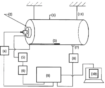
FIG. 1. Experimental setup. (1) cylindrical shell, (2) acoustic driver (loud-
speaker), (3) microphone, (4) microphone power supply, (5) power supply, (6) white-noise source, (7) accelerometer, (8) charge amplifier, (9) FFT ana-
lyzer, (10) personal computer, (11) elastic string.
where [(ro) is the FRF between the signals fi and •Y. If the same loudspeaker is used for all measurements of the FRFs,
the overall FRF matrix between the pressure and displace-
ment is then
Yxp-YxuY•-u•-(1/iYx•)(iY•-)):Yx•Y•-•
•,
(22)
where
the submatrix
Yxv is associated
with .•i/fij and the
submatrix
Ypv is associated
with/5i/•j, and
each
entry
of the
FRFs can easily be measured by the voltage source. Substi-
tuting Eq. (22) into Eq. (19) gives
:VxvV;2fi.
(23)
From
Eq. (23), the FRF submatrices
Yx• and Yp• can be
used
to estimate
the acoustically
induced
vibrations.
Note
that inversion
of Yp• does
not have
ill-conditioned
problems
since it is directly measured and is generally full rank. In addition, the coupled system technique does not require the system of interest to be weakly coupled nor in resonance.
II. EXPERIMENTAL INVESTIGATION
Figure 1 shows the experimental setup and instrumenta- tion. A steel cylindrical shell of length 1 m, radius 0.2 m, and
thickness 2 mm is selected to verify the developed tech- niques. The ends of the cylindrical shell are covered with
steel plates and the closure is done by screws and tapes to ensure air tightness and vibration suppression. The shell is
freely suspended by elastic strings. A 4-• and 30-W loud-
speaker is attached on the top cover of the shell to serve as an acoustic source. Sound pressure and surface acceleration are measured with a 1/2-in. condenser microphone and an
11-g accelerometer, respectively. It should be noted that in the following experimental results the source points used to generate the response curves were all different from the points used to measure the acoustic pressure under point
force mechanical excitation.
cavity
P•
mi½. V
'1
Audspeaker
FIG. 2. The convertible acoustic driver.
A. The resonant system technique
This method requires the measurement of volume accel-
eration
of the acoustic
source
to determine
Yxu or Ypu. To
this end, a convertible acoustic driver 21'22 is mounted on the top of the cylindrical shell to excite the internal acoustic field
(Fig. 2).
To calculate the mode shapes of the coupled system, it suffices to measure only one column or one row of the FRF
matrix. Figure 3 shows 32 DOFs for the FRF measurement,
including the structural DOFs 1-30 and the acoustic DOFs 31 and 32 located on the external and the internal surfaces of
the shell, respectively. The volume acceleration excitation is applied to the acoustic DOF 31 so that a set of FRFs Y i31,
i= 1-32 can be measured (Yi31, i= 1-30 correspond to Yxu
and
Y i31, i-31, 32 correspond
to Ypu).
From
the measured
FRFs, the natural frequencies and mode shapes of thecoupled system can be calculated by the forgoing curve- fitting procedure.
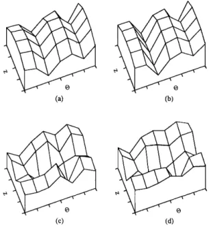
An experiment is performed to verify this method. The cylindrical shell is subjected to sinusoidal acoustic excita- tions at the resonant frequencies 323 and 385 Hz, by using a
loudspeaker located inside the shell at a position different
Unit: mm
•
F-too
32 • •>6 > • "' 26 I 11 16 21 2 7 12 17 22 27 ) ' • • , 3 8 13 18 23 28•4 19 14
19
i24
'29
i'5 10 t• 20 '25 •30FIG. 3. The DOFs on the cylindrical shell defined for the resonant system technique. (3: structural DOF, [3: acoustic DOF.
(c) (d)
FIG. 4. Displacement amplitudes of all structural DOFs for the resonant frequencies 323 and 385 Hz estimated by the resonant system technique in
comparison with the measured data. (a) Estimated data at 323 Hz; (b) mea-
sured data at 323 Hz; (c) estimated data at 385 Hz; (d) measured data at 385
Hz.
from the original one. Then, based on the extracted mode shapes, the surface displacements at the resonant frequencies are estimated by the measured pressure at the acoustic DOF 32. Figure 4 compares the estimated displacements with the
measured data for each structural DOF. The results appear to
be in good agreement except for some discrepancies because
of numerical errors of curve fitting.
Unit: mm
[] [] []
4 5 6 " i
o
I
FIG. 5. The DOFs on the cylindrical shell defined for the coupled system technique. O: structural DOF, [] acoustic DOF.
acoustic DOF. The sound pressures • and the FRF submatri-
ces
Yxu
and
Ypu
are substituted
into
Eq. (19) to calculate
the
displacements • at each frequency.
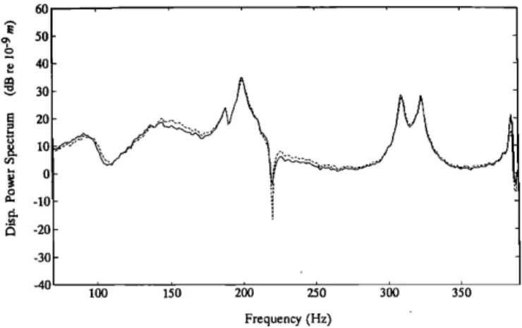
Figure 6 compares the estimated and the measured dis-
placement power spectra of the structural DOF 1. It can be seen from the result that significant error occurs due to rank
deficiency
of Ypu. This can
be alleviated
by SVD pseudoin-
version. The calculated result in Fig. 7 appears better thanthat obtained
from direct
inversion
of Ypu in Fig. 6.
Next, the method of direct FRF measurement is applied to the same test case. As can be observed in the experimental
result of Fig. 8, the estimated displacement power spectrum
is in excellent agreement with the measured spectrum be- cause this approach essentially eliminates the rank-
deficiency
problem
of Ypu.
B. The coupled system technique
As mentioned earlier, two methods are available for ob-
taining
the FRF submatrices
Yxu and Ypu required
by this
method. One may construct the modal model of the coupled system, based on only one column of FRF measurements, and partition the resulting FRF matrix. Alternatively, onemay directly measure the full FRF matrix without curve-
fitting. In the following case of FRF measurement, six DOFs (including the structural DOFs 1 and 2 and the acoustic DOFs 3-6) are defined for the cylindrical shell, as shown in
Fig. 5. Hence,
the Yxu and Ypu are 2x4 and 4x4 matrices,
respectively.
When the first method is employed, one column of the FRF matrix is measured by using the volume acceleration source acting on DOF 3. By curve-fitting the FRFs in the frequency range 70-390 Hz, the modal parameters are cal- culated. Then, the modal model of the coupled system is constructed from the extracted modal parameters.
Alternatively, when the full FRF matrix is directly mea- sured by using Eq. (22), the voltage signal driving the loud-
speaker
is taken
as the
•xcitation.
The
FRFs
y ij between
the
excitation
position
j •(voltage
signal)
and
the response
posi-
tion i (displacement or'pressure) are measured.
In this experiment, a loudspeaker is located at the acous-
tic DOF 3. The sound pressures • are measured at each
III. CONCLUSION
Two experimental techniques have been developed to
estimate shell vibrations induced by internal acoustic pres-
sure. Experiments are conducted on a steel cylindrical shell
to verify the proposed methods. The surface vibrations esti- mated by these methods are found to be in good agreement with the measured data.
50 30 20 lO o -10 -20 -30 -40 160 1•0 260 2•0 360 3•0 Frequency (Hz)
FIG. 6. Displacement power spectrum of DOF 1 estimated by the coupled
system technique based on the derived modal model with four acoustic DOFs. --, estimated data; --- measured data.
•' 50 ? ß - 40 • 30 • 20 • •o o •. 40 t3 -20 -30 -40 100 150 200 250 360 3}0 Frequency (Hz)
FIG. 7. Displacement power spectrum of DOF 1 estimated by the coupled system technique based on the derived modal model with four acoustic
DOFs. Pseudoinversion of Yp, is calculated by SVD. •, estimated
data; --- measured data.
From the experimental results, some remarks are in or- der. The advantage of the resonant system technique is that it provides satisfactory estimations for the acoustically induced vibration at resonant frequencies. Its disadvantages, on the other hand, are that (i) it is not applicable to nonresonant frequencies and (ii) one need construct a volume acceleration
source
for FRF measurement.
The advantages
of the coupled
system technique are that (i) it provides accurate estimations for the acoustically induced vibration, (ii) it has less fre-quency limitation than the other two methods, and (iii) its
experimental procedure is simple to apply. The disadvantage of this method lies in the fact that the data-acquisition pro- cedure appears somewhat tedious if direct FRF measurement
is employed.
The experimental techniques are well suited for the ap- plications where structural vibrations induced by internal
60 . 50 40 30
ø
-20 -30 40 100 150 200 250 300 350 Frequency (Hz)FIG. 8. Displacement power spectrum of DOF 1 estimated by the coupled system technique based on direct FRF measurement with four acoustic
DOFs. •., estimated data; --- measured data.
acoustic fields are desired, but direct measurement of vibra-
tions is not feasible. For complex problems where analytical
or numerical approaches are prohibitive, the proposed ex- perimental techniques serve as simple but useful alternatives.
ACKNOWLEDGMENT
The work was supported by the National Science Coun- cil in Taiwan, Republic of China, under Project No. NSC-81- 0401-E009-571.
l w. H. Clark, "Experimental Investigation of Pressure Oscillations in A Side Dump Ramjet Combustor," AIAA J. 19, 47-53 (1982).
2V. Yang and F. E. C. Click, "Analysis of Low Frequency Combustion Instabilities in a Laboratory Ramjet Combustors," Combust. Sci. Technol. 45, 1-25 (1986).
3 A. Craggs, "The Transient Response of A Coupled Plate-Acoustic Sys- tem Using Plate and Acoustic Finite Elements," J. Sound Vib. 15, 509- 528 (1971).
4D. J. Nefske, J. A. Wolfe, and L. J. Howell, "Structural-Acoustic Finite
Element Analysis of the Automobile Passenger Compartment: a Review of Current Practice," J. Sound Vib. 80, 247-266 (1982).
5 j. D. Jones and C. R. Fuller, "Influence of a Floor on Sound Transmission
into an Aircraft Fuselage Model," J. Aircraft 25, 882-889 (1988). 6F. J. Fahy, "Vibration of Containing Structures by Sound in the Contained
Fluid," J. Sound Vib. 10, 490-512 (1969).
7A. C. Fagerlund and C,• D. Chou, "Sound Transmission through a Cylin- drical Pipe Wall," ASME Trans. J. Eng. Ind. 103, 355-360 (1981). 8F. J. Fahy, Sound and Structural Vibration: Radiation, Transmission and
Response (Academic, London, 1985).
9E. H. Dowell, G. F. Gorman, and D. A. Smith, "Acoustoelasticity: Gen- eral Theory, Acoustic Natural Modes and Forced Response to Sinusoidal Excitation, Including Comparisons with Experiment," J. Sound Vib. 52,
5i9-542 (1977).
•øM. P. Norton, Fundamentals of Noise and Vibration Analysis for Engi-
neers (Cambridge U.P., New York, 1989).
•D. J. Nefske and S. H. Sung, "Component Mode Synthesis of a Vehicle Structural-Acoustic System," AIAA J. 24, 1021-1026 (1986).
12j. M. Shippen and J. W. Dunn, "Selective Elasto-Acoustic Modal Synthe-
sis by Orthogonallty Criteria Applied to Vehicle Structures," J. Vehicle
Des. 12, 208-216 (1991).
•3 Z. D. Ma and I. Hagiwara, "Improved Mod•-Superposition Technique for Modal Frequency Response Analysis of Coupled Acoustic-Structural Sys- tems," AIAA J. 29, 1720-1726 (1991).
•4Z. D. Ma and I. Hagiwara, "Sensitivity A•alysis Method for Coupled
Acoustic-Structural Systems Part I: Modal Sensitivities," AIAA J. 29, 1787-1795 (1991).
•SD. J. Ewins, J. M. M. Silva, and G. Maleci, "Vibration Analysis of a
Helicopter with an Externally Attached Carrier Structure," Shock Vib. Bull. 50, 155-171 (1980).
•6D. J. Ewins, Modal Testing: Theory and Practice (Research Studies, En- gland, 1985).
•7 H. G. D. Goyder, "Methods and Application of Structural Modeling from Measured Structural Frequency Response Data," J. Sound Vib. 68, 209- 230 (1980).
laD. L. Brown, R. J. Allemang, and M. Mergeay, "Parameter Estimation Techniques for Modal Analysis," SAE Paper No. 790221, 1979, pp. 526-
544.
19D. J. Ewins and P. T Gleeson, "A Method for Modal Identification of Lightly Damped Structures," J. Sound Vib. 84, 57-79 (1982).
2øB. Noble and I. W. Daniel, Applied Linear Algebra (Prentice-Hall, Engle- wood Cliffs, NJ, 1988).
2• R. Singh and M. Schary, "Acoustic Impedance Measurement Using Sine Sweep Excitation and Known Volume Velocity Technique," J. Acoust. Soc. Am. 64, 995-1003 (1971).
22 C. H. Kung and R. Singh, "Experimental Modal Analysis Technique for Three-Dimensional Acoustic Cavities," J. Acoust. Soc. Am. 77, 731-738
(1985).