國 立 高 雄 應 用 科 技 大 學
電 子 工 程 系 碩 士 班
碩 士 論 文
啟發式最佳化方法應用於智慧電網之配置與管理
Configuration and Management of Smart Grids with Heuristic
Optimization Methods
研 究 生: 里橋爾
指導教授:
謝欽旭 博士
洪盟峯 博士
中華民國一 O 五年七月
啟發式最佳化方法應用於智慧電網之配置與管理
Configuration and Management of Smart Grids with Heuristic
Optimization Methods
研究生 :里橋爾
Rijal Achmad
指導教授 :謝欽旭 博士
洪盟峯 博士
Dr. Chin-Shiuh
Shieh
Dr. Horng
Mong-Fong
國立高雄應用科技大學
電子工程系碩士班
碩士論文
A Thesis Submitted to
Department of Electronics Engineering
National Kaohsiung University of Applied Sciences
in Partial Fulfillment of the Requirements
for the Degree of Master
in
Electronic Engineering
July 2016
Kaohsiung, Taiwan, Republic of China
Configuration and Management of Smart Grids with Heuristic Optimization Methods
Student: Rijal Achmad Advisor: Dr. Chin Shiuh Shieh Dr. Horng Mong-Fong Department of Electronics Engineering
National Kaohsiung University of Applied Sciences
ABSTRACT
With the depletion of fossil fuels, the use of renewable energy has become the nifty option to meet the energy demand. In order to meet the high load demand the use of renewable energy could be optimized, however, the renewable energy naturally is out of human control since the nature of renewable energy such as the wind and solar energy is uncertain. The hybrid system could be a well alternative to support the use of renewable energy.
Using probability density function and sampling to define Estimation Point of the source, this study will examine the probability of generating power in the grid system including the management energy system between the source and the demand as well. The evolutionary algorithm such as Genetic Algorithm will be used to execute the optimization decision value for the optimal capacity size.
The proposed method will present the solution of renewable energy more efficiently and in balance. The non-one-sided energy generation would support each other in the system as well. The variance of the load shifting as the demand management will show in various rate includes the generation sizing. The flexibility of the system which affects the capacity decision of the hybrid system is also assessed.
Keywords: Evolutionary Algorithm, Hybrid System, Energy Management, Renewable Energy, Optimization.
ACKNOWLEDGEMENTS
In the name of Allah, the Most Gracious and the Most Merciful Alhamdulillah, all praises to Allah for the strengths and His blessing in completing this thesis. It is a great pleasure to acknowledge my deepest appreciation and greatest gratitude to my advisors Professor Chin-Shiuh Shieh to guide in my research. He has a significant contribution in this research. With his immense knowledge he the give numerous suggestions and push me to think in a broader way in order to make the research better.
I extend my special gratitude to Professor Mong-Fong Horng as the second parent in school, for his patience and motivation. He provided insight and expertise that greatly supported the research. His direction assists me in all the time to completed this research.
Next, I would like to express great thanks Professor Mu-Liang Wang. As committee member he helps to make my thesis better. He gives his best attention in my research.
Not less important, I would like to show deeply grateful to Professor Yuh-Chung Lin, to help me improve my writing and correct many grammatical mistakes in my writing with his great enthusiasm.
I also acknowledge with a deep sense of honor, my gratitude towards my parents and member of my family for the support they devote to me through in my whole life and in particular.
Finally, but not the end of my gratefulness is to all of my friends, lab 702, and senior brother who help me directly or indirectly, also motivated me to completed this master thesis.
Rijal Achmad Department of Electronics Engineering July 2016
CONTENT ABSTRACT ... i ACKNOWLEDGEMENT ... ii CONTENT ... iii LIST OF TABLES ... v LIST OF SYMBOLS ... v LIST OF FIGURES... vi CHAPTER 1 INTRODUCTION 1.1 Background ... 1
1.2 Hybrid Renewable Energy ... 2
1.3 Load Shifting and Power Management Method ... 5
CHAPTER 2 LITERATURE REVIEW 2.1 Modelling method ... 11
2.1.1 Wind Probabilistic Generation Modeling ... 11
2.1.2 Solar Probabilistic Generation Modeling ... 16
2.2 Optimization Problem, Classical Numerical Methods
and Deterministic Approaches ... 21
2.3 Heuristic Optimization ... 27
2.3.1 Genetic Algorithm ... 30
2.3.2 Differential Evolution ... 33
CHAPTER 3 PROPOSED METHOD 3.1 Model Description ... 40
3.2 Deterministic Approach ... 55
3.3 Stochastic Approach Genetic Algorithm... 57
3.4 Stochastic Approach Differential Evolution ... 59
CHAPTER 4 RESULT 4.1 Result of Optimal Component Sizing ... 61
4.2 Result of Additional Balancing System ... 62
4.3 Result of Different Charging/Discharging Rate of Storage System... 64
4.4 Deterministic Result with Classical Approach ... 66
4.5 Comparative Result Between GA and DE ... 68
CHAPTER 5 CONCLUSION AND FUTURE WORK ... 73
LIST OF TABLES
Table 1. Result Without Balance of Energy Supply in Genetic Algorithm . . 62 Table 2. Result with Balance of Energy Supply in Genetic Algorithm ... 64 Table 3. Result with Different Rate of Storage Charging and Discharging 65 Table 4. Deterministic Component Sizing with Mixed Integer Non-Linear
Programming ... 67 Table 5. Genetic Algorithm and Differential Evolution Parameter Setting... 68
LIST OF SYMBOLS
α = Shape Parameter
β = Scale Parameter
µ = mean value
σ = standard deviation
v = Wind Speed Bin (m/s)
vi = Cut in Speed (m/s)
vr = Rated Output (Watt)
v0 = Cut out Speed (m/s)
kt = Solar Radiation Bin (Watt)
H = Total Solar Radiation (Watt)
r = Solar Panel efficiency yield (%)
A = PV Surface (m2)
Pw = Power Output (MW)
Pw r = Generator Rating (MW)
Ew = Cost for Each Installed Wind Scale
($)
Epv = Cost for Each Installed
Solar Scale ($)
IEw = Installation Cost of Wind
Generation ($)
IEpv = Installation Cost of PV
Generation ($)
IEs = Installation Cost of Storage System ($)
OEw = Operation Cost of Wind
Generation ($)
OEpv = Operation Cost of PV
Generation ($)
OEs = Operation Cost of Storage
($)
αw = Installed Wind Rating Power
αpv = Installed Solar Rating
Power
S = Installed Storage Capacity (MW)
EP = Power Rating Cost ($)
P = Power Rating (MW)
Ppv = Estimation Number of Solar Power (MW)
Pwt = Total Wind Output
Generated (MW)
Ppvt = Total Solar Output
Generated (MW)
Lv = Load Variance (MW)
ES = Energy Surplus (MW)
Lmin = Minimum load should have
covered (%)
Sc = Storage Capacity (MW)
d = Charging/Discharging Rate Value
(%)
ηs = Efficiency of Storing (%)
Lst = Load Shifting (MW)
LIST OF FIGURES
Fig 1. Hybrid storage system ... 4
Fig 2. Load shifting illustration ... 6
Fig 3. Interconnection in smart grid ... 8
Fig 4. Architecture of home energy management ... 9
Fig 5. The Weibull Data Plot ... 13
Fig 6. Wind speed distribution illustration ... 14
Fig 7. Wind Turbine Power Output Characteristic ... 15
Fig 8. Illustration of Beta Distribution Shape ... 18
Fig 9. Typical I - V characteristic of a photovoltaic cell ... 19
Fig 10. Global and Local Optima Illustration ... 22
Fig 11. Crossover Process Illustration Using 6 Variable Dimension ... 38
Fig 12. Hybrid Renewable System in Smart Grid Interconnection ... 40
Fig 13. Flowchart Proposed Optimization Method in GA ... 42
Fig 14. Fitting Wind Distribution ... 43
Fig 15. Fitting Solar Distribution ... 44
Fig 17. Ideal Energy Generation Planning ... 50
Fig 18. Storage Sizing Illustration ... 52
Fig 19. Illustration of Modified Load in the Load Variance ... 53
Fig 20. The Mixed Integer Non-Linear Programming Process... 50
Fig 21. The Real Value GA Chromosome Example ... 57
Fig 22. The Genetic Algorithm Process ... 58
Fig 23. Differential Evolution Applied Vector ... 59
Fig 24. The Differential Evolution Process ... 60
Fig 25. Minimum Total Expense GA and DE ... 69
Fig 26. PV Scale Component Sizing with Variance of Load Shifting Rate 70
Fig 27. Wind Scale Component Sizing with Variance of Load Shifting Rate 71 Fig 28. DE and GA convergence characteristic... 72
CHAPTER 1 INTRODUCTION
1.1 Background
The increase of energy demand makes energy management becomes important in nowadays, the high demand with limited energy source would be a problem to deal with it. On the other hand, the use of fossil fuel as the main energy source should have limitations or even have to reduce to avoid the depletion of fossil fuel [1], the fossil fuel availability needs many decades to regenerate and able to reuse again.
More than 65% electricity power in the world supplying the energy demand nowadays is produced by steam turbine power plant heating fossil fuels as an energy source. And the immense number of fossil-fueled power plants supply the most of the world's load generating capacity. The Fossil fueled power plants which use coal, oil or gas in order to ignite the incineration chambers to heat the steam. All of them are non-renewable resources which supply will eventually be depleted.
Oil fuel might be highly convenient fuel, roughly three decades before it contributed 30% energy to supply demand, however, mostly it has been substituted with coal because the oil expense has increased more rapidly than the coal price as to insecurity of availability source. At that time, the primary use of oil fuel for run the transportation and chemical purposes than only burn to extract the oil calorific value has also already been discovered.
and carrying the coal is more troublesome moreover the coal inflicts huge numerous of residues, greenhouse gasses and ash, that kind of them are toxic matter, this problem is depending on the kind of coal quality.
Consider the three conversion work, mechanical, and thermal, become electrical energy, the essence energy used from the fossil fuels and the overall efficiency of fossil fueled generated power plant roughly about 40 percent. This evidence means the 60% of the input energy is wasted in the power plant system. Therefore, the efficiencies of the conversion probably low as 30 percent in several conventional power plants. All of power generation are not similar, the proper efficiencies achieved rely on the fuels use and the technique of the generate plant and processes.
1.2 Hybrid Renewable Energy
Because of the first time problems appeared in this thesis, the use of renewable energy such as photovoltaic (PV), wind, biomass, fuel cell, micro-hydro, etc. become a nifty alternative to overcome the increasing energy demand. For example, in practically Grid-connected systems are dimensioned for average wind speeds 5.5 m/s on land and 6.5 m/s offshore where wind turbulence is less and wind speeds are higher. While offshore plants benefit from higher sustainable wind speeds, their construction and maintenance costs are higher. Large-scale wind turbine generators with outputs of up to 8 MW or more with rotor diameters up to 164 meters are now functioning in many regions of the world with even larger designs in the pipeline [22].
However, the reliability of some renewable energy is cannot exactly guarantee because uncertain generation output often did not match the demand pattern [2, 3]. For
example, the wind turbine is depending on wind speed to rotate the turbine, sometimes when the wind has enough speed to produce huge output but less load demand the rest of energy will be discarded. In this situation the hybrid system utilizes with storage system could be useful to overcome the problem. When the energy sources are abundant and the demand is less the energy surplus will save on the storage and then can be released when demand increase and need additional supply energy.
Hybrid renewable energy systems consist of two or more renewable energy products such as solar PV panels, wind generators, Hydro generators, etc. There is a dramatic increase in energy production when hybrid systems are installed typically because multiple renewable energy sources are being utilized. For example, a solar and wind hybrid system provides the advantage of sunny quiet days to produce energy from sunlight while cloudy windy days provides energy directly from the wind [21]. This is the most popular renewable energy hybrid system because it provides energy generation during most weather conditions. Hybrid systems can be installed to operate as either on the grid or off-grid system making them popular in almost all renewable energy installations.
Mostly in the United States, the wind velocities are less in the summer, at the same time the solar irradiance was immense. In the winter the wind is strong while sunlight is less available. Because the peak generating period for the wind and photovoltaic systems develop at different times, the hybrid systems are likely to generate more power when you need it.
Most of the hybrid systems are independent systems, which perform off the grid (not connected directly to an electricity distribution system). In this situation when neither the wind nor the solar system is producing, many hybrid systems supply energy by the batteries and/or a conventional engine generator powered.
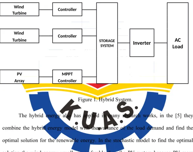
Wind Controller STORAGE SYSTEM AC Load Turbine Wind Controller Inverter Turbine PV MPPT Array Controller
Figure 1. Hybrid System.
The hybrid energy also has applied in many research works, in the [5] they combine the hybrid energy model with the variance of the load demand and find the optimal solution for the renewable energy. In the stochastic model to find the optimal solution the wind energy usually is preferable than the PV system because PV more expensive. Even the energy resources have the same energy potential output, the price of the PV to produce same output will cost higher. The additional method will implement to make the power system more balance. This method will be useful for some places which have both of potential energy, for example when the wind on the day
is limited and the solar energy is available, there will be good results to take advantages of solar power to supply the insufficient wind.
1.3 Load Shifting and Power Management Method
The process to transfer the high energy block is called by Load Shifting. It moves those energies use during a period of time by move forward or postpones their use until the energy supply system can fulfill the extra load readily, the illustration of load shifting can see in figure 2. The conventional purpose behind this process is to reduce generation capacity requirements by adjusting load variance. When the loads difficult be arranged, this should be carried out by implementing energy storage systems to move the load pattern as mentioned in the hybrid system.
By implementing an energy storage system, it is also possible to alternate the varied demand into one with a relatively equal and consistent output. For instance, the great-scale installation of renewable energy generation coupled with the Smart Grid relies highly on energy storage systems for maximum effectiveness and optimization.
Depending on the application, peak-load shifting can be referred to as peak shaving or peak smoothing. As an example, in the night, the energy storage system is charged while the electrical supply system is powering minimal load and the cost of electric usage is reduced. It is then discharged to provide additional power during periods of increased loading, while costs for using electricity are increased. This operation also able to applied to decrease electricity invoice, and also effectively change
the high load demand effect on the system, by minimizing the generation capacity required [20].
Object 69
Figure 2. Load shifting illustration.
Load shifting is not a new concept and has been applied successfully in the past by users in many industrial and great-scale commercial facilities to reduce electrical
peak demand which affects energy bills. However, there are some problem implement load shifting in conventional power plants. First, during operating conditions, it is difficult to start and stops the production. It means generators should be work continuously. Start and stopping will make maintenance costly and hard, in addition also have the flexibility limitation of the power plant. Second, Unmatched with load demand pattern, the overage steam will be released during the off-peak period, indeed wasting energy and fuel. Third, peaking power plants which only perform during peak energy demand hours will not use for 90% of the time. This disadvantage indicates the failure of conventional energy to meet the deep slopes of the load curve. Fourth, when having low-quality coal many power plants will operate under their actual capacity, this conditions will make difficult to arrange the exact coal input to match with load demand as well.
With the rapid expansion of renewable energy plants in recent years, peak-load shifting has received significant concern. Renewable energy sources especially the winds and photovoltaics (PV), has observed exponential development recently, provide irregular power due to meteorological and atmospheric conditions. As these power generations arrive to supply an increasingly notable contribution to the load demand on the electrical grid, their effects become more pronounced on the power quality of that grid. The uncertain fluctuations in power generated by these renewables can be difficult to maintaining transient and dynamic stability within the system. Power quality concerns generally associated with renewable energy sources include voltage transients, frequency deviation, and harmonics.
The advanced of information technology era would enhance the use of smart grid and help to organize the power system much better, illustrated in figure 3. Smart grid is a modernized electrical system grid that uses digital information and communications technology to gather and act on information, such as information about the behaviors of suppliers and consumers, in an automated fashion to improve the efficiency, reliability, economics, and sustainability of the production and distribution of electricity.
Figure 3. Interconnection in smart grid. (source: https://www.knowstartup.com).
Modernized electrical grid with the communication system has established the power scheduling method in home energy management system. That method utilizes cutting edge information and communications technology built in smart grid system would effectively decrease peak of average rate of energy use [4]. The utility combination including AMI (Advanced Metering Infrastructure) deployed in the home energy management system cooperate with home gateway and the integrated grid itself make the load management more flexible and reliable. The AMI responsible for collecting and transmitting power meter reading, pre-payment, tariff to the utility
company as well. The figure 4 showed the component of AMI itself is Smart Meter, Home Gateway, and In Home Display.
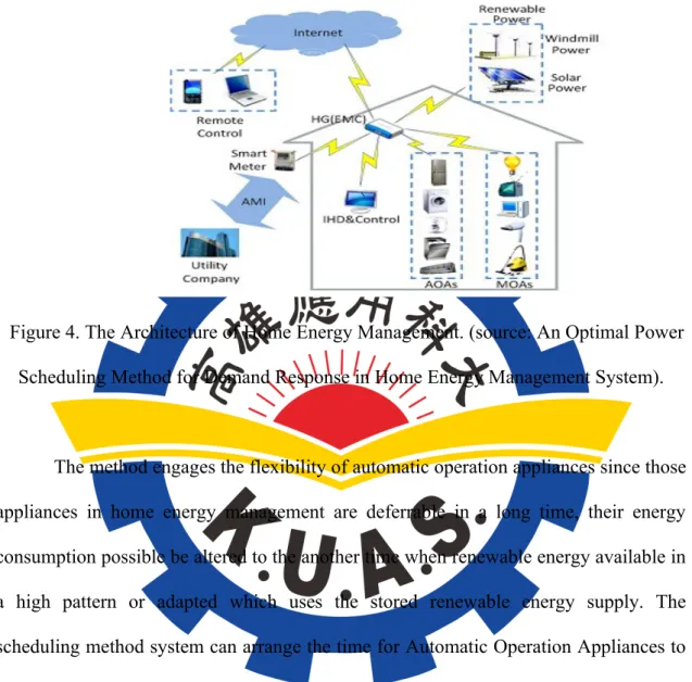
Figure 4. The Architecture of Home Energy Management. (source: An Optimal Power Scheduling Method for Demand Response in Home Energy Management System).
The method engages the flexibility of automatic operation appliances since those appliances in home energy management are deferrable in a long time, their energy consumption possible be altered to the another time when renewable energy available in a high pattern or adapted which uses the stored renewable energy supply. The scheduling method system can arrange the time for Automatic Operation Appliances to operate and send the information to the network whether the system needs necessary additional energy or not and give information about the availability of reserved energy. Theoretically, combining the power management method in home energy management and energy management function in hybrid storage system the average peak energy demand rate could be reduced and the energy use will be more effectively distribute.
The work for the scheduling load demand has to show positive result to manage the peak of load demand, the methodology to move the high load to the other time slot was effectively decrease peak of energy demand average rate and give the low tariff pricing for the resident. Those methods would give advantages when co-operating with another method to optimize the work of renewable energy. In this research the shifted load in power scheduling method will be implemented as the load shifting, the flexibility of the load shifting could affect the power generation and storage system component sizing as well.
In the proposed scenario of [5] the optimization of the wind and solar generation capacity is tending to obtain the optimal solution for the wind or the solar, however in this paper is try to obtain the balance optimization between the wind and solar to fulfill load demand. In some places which have both of energy resources, the balance of optimal capacity will significantly useful, those renewable power source could support each other when the day have a lot solar but low velocity of the wind, the solar system will helpful for supply demand and vice versa.
The additional advantage of utilizing the storage system is to save the discarded energy as reserved energy, and then the reserved energy can discharge back to the system when the load is conges [8, 11, 12]. With those systems, the potential capacity factor both for wind and solar can be unconstrained. The larger storage capacity will make the effective capacity factor increase as the potential of wind and solar pushed into full factor. However, it will give big cost factor, power duration, and congestion duration. From those consider the cost, size from the renewable energy, the charging/discharging rate, and load shifting planning should be developing in balance.
CHAPTER 2 LITERATURE REVIEW
2.1 Modeling Method
The generation of the wind and solar power is cannot decide by ourselves, it is depending on the nature behavior to produce such a wind speed and solar irradiation index. Due the dependent input that affects the power generation output, we should forecast the wind and solar behavior or rather use historical data and model it. To model the wind and solar generation output we can use probability density function. The historical data is needed to achieve the pattern of distribution, after determining the pattern of wind and solar from clustering the historical data, the curve fitting should be useful to attain the scale factor and shape parameter of the pattern. Probability density function could be suitable to model the probability of wind velocity and solar radiation. The variable that affects the pattern of distribution is turned as parameters for generating the pseudo random number which resembles the wind speed and solar irradiation data identically [7].
2.1.1 Wind Probabilistic Generation Modeling
Weibull distribution is a suitable use of modeling probability of wind pattern speed. In the statistical theory and probability technique, the Weibull distribution is one of the widest use, reliable, and continuous probability distribution. Due to its versatility, the Weibull distribution can be used to model a variety of life behaviors. Those advantages have made it highly recommended probability modeling technique for engineers and scientists who used distribution for modeling reliability data. The Weibull
distribution can easily integrate into their data analysis because it is quite flexible to model most of the datasets [18].
The main function uses Weibull distribution function is the able to provide reasonably accurate forecasts and failure analysis in really small sample samples. The solutions are possible become indications of a problem at the earliest without having to simulate many times, moreover taking samples would also consider cost-effective component testing. For instance, when having test for four bearings the unpredictable Weibull tests are completed when the first failure evidence in every group of components. Imagine if all of the bearings should be tested to failure manually, the expense and time required is much greater [19].
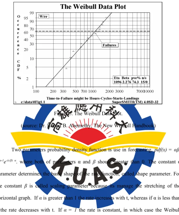
The other advantages of Weibull are it have a simple and beneficial graphical plot of the failure data. the engineer is highly recommended to use the data plot. The data plot of Weibull is especially rich of information as Waloddi Weibull explained out on his paper in 1951’s. In the figure 5 show the Weibull plot characteristic that firstly introduce. The horizontal scale is a measure of life or aging. Start/stop cycles, mileage, operating time, landings or mission cycles are examples of aging parameters. The vertical scale is the cumulative percentage failed. The two defining parameters of the Weibull line are the slope, beta, and the characteristic life. The slope of the line, β, is particularly significant and may provide a clue to the physics of the failure [19].
Figure 5. The Weibull Data Plot.
(source: Dr. Robert B. Abernethy, The New Weibull Handbook)
Two parameters probability density function is use in forecasting, pdf(x) = αβ -αxα-1e-(x/β) α. where both of parameters α and β should greater than 0. The constant α
parameter determines the basic shape of the rate function, called shape parameter. For the constant β is called scaling parameter because its manage the stretching of the horizontal graph. If α is greater than 1 the rate increases with t, whereas if α is less than 1 the rate decreases with t. If α = 1 the rate is constant, in which case the Weibull distribution equals the exponential distribution. In the wind probability modeling we use the 1-parameter Weibull, the 1-parameter Weibull pdf is obtained by setting α = 0 and assuming β as constantly assumed value. The α as a shape parameter and β as scale parameter.
(1)
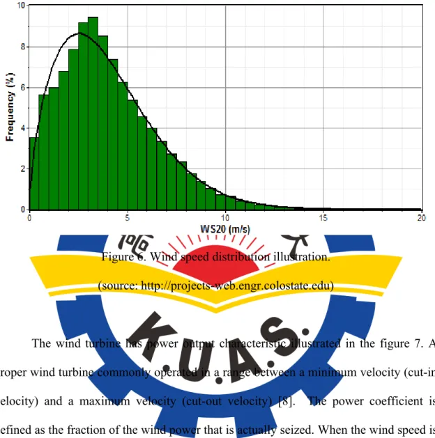
Figure 6. Wind speed distribution illustration. (source:http://projects-web.engr.colostate.edu)
The wind turbine has power output characteristic illustrated in the figure 7. A proper wind turbine commonly operated in a range between a minimum velocity (cut-in velocity) and a maximum velocity (cut-out velocity) [8]. The power coefficient is defined as the fraction of the wind power that is actually seized. When the wind speed is below cut-in speed the power output is 0. The wind turbine generator has the limitation of the power generation. When the potential output power of the wind turbine is more than the maximum input power to the generator, the turbine is controlled to adjust output only the maximum generator power. This function equipped with attached braking system is to maintain the wind turbine standstill, when the velocity increases
above the rated output wind velocity, the force on the turbine will continue to extend and at some point there is a risk to break the rotor.
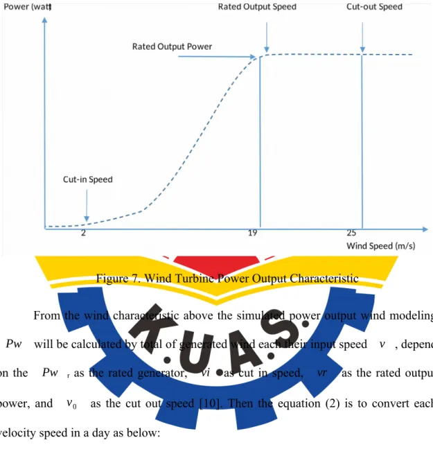
Figure 7. Wind Turbine Power Output Characteristic
From the wind characteristic above the simulated power output wind modeling Pw will be calculated by total of generated wind each their input speed v , depend on the Pw r as the rated generator, vi as cut in speed, vr as the rated output power, and v0 as the cut out speed [10]. Then the equation (2) is to convert each velocity speed in a day as below:
Pw=
{
0 v−vi vr−vi Pwr Pwr v ≤ vi , v ≥ v0 vi≤ v ≤ vr vr ≤ v ≤ v0 (2) where: Pw = Power Output (MW)Pw r = Generator Rating (MW)
v = Wind Speed (m/s)
vi = Cut in Speed (m/s)
vr = Rated Output Power (MW)
v0 = Cut-out Speed (m/s)
2.1.2 Solar Probabilistic Generation Modeling
In the next probability distribution function, we use beta distribution to achieve the pattern probabilistic of solar irradiance. Similar to Weibull distribution, the beta distribution also has been applied to model the behavior of random variables limited to intervals of finite length in a wide variety of disciplines. The beta distribution is a suitable model for the random behavior of percentages and proportions.
The basic form of Beta distribution similar to Gamma distribution. The distribution can be an alternative to consider for variables that naturally tend to extremely inclined. When the random variable Y is gamma distributed with parameters
α and β, then the likelihood of Y is given by:
p (Y )= β
α
Г (α)Y
α−1
e−βY, Y ≥ 0 , β>0 , α>0 (3)
thus the function of gamma Γ (x) will be defined as below:
Г ( x )=
∫
0 ∞
where x is a complex variable and Re(x) > 0. In this form, the function called as Euler’s integral form Gamma function. Similar with the lognormal function distribution, the Y value and the parameters α and β should be positive value. The α parameter defined as the shape parameter. The β parameter is defined as the inverse parameter scale. As an example, the standard deviation in the gamma distribution is comparable with 1/β. The mean value of gamma distribution variable is α divided β. And the variance value would be α / β2. When α larger than 1, then there is a mode which is (α-1) / β. The first form of Beta distribution is given by:
f ( x ;α , β )= 1 B (α , β )x
α−1(1−x )β −1
(5)
where the α and β parameters are defined as positive real value and the x variable should satisfy 0 ≤ x ≤ 1. Then the Beta function value B( α , β ) as the dominant factor run the function as normalizer constant which makes sure that the sum of all area within the density curve equivalent 1 value. Thus the Beta function is defined as a ratio of general Gamma functions as:
B ( α , β)=Г (α) Г (β ) Г (α +β)
(6)
where α=β=1 the Beta distribution simply becomes a uniform distribution with range between 0 and 1. Where α=1 and β=1 or vice versa we obtain triangular shaped distributions, when f(x) = 2 − 2x and the f(x) value is 2x. When α=β=2 we would obtain the parabolic distribution shape f(x) = 6x(1− x). Generally, when both α and β are larger than one the distribution has a specific characteristic at x = (
α − 1)/( α + β − 2) and is zero at the last points. When α and/or β is
less than one f(0) would be infinity, or when f(1) → ∞ the distribution is resulted to be J shape.
The beta distribution is also categorizing as a continuous distribution which also has two parameters α and β, however, both is referred to as shape parameters (shape1 and shape2 in x). If we want to model the solar irradiance with the expected number of a variable that is beta distributed we also can directly use equation defined below:
E ( x )=μ= α
α +β (7)
And if we need to model the variance from a beta distribution will be as below:
Variance ( x)= αβ
( α + β )2(α + β +1) (8)
The radiation value generation kt statistically is modeled using probability density function of beta distribution. Thus the probability density function Fci
(
kt)
that uses to generate random number variable in curve fitting is below:Fci
(
kt)
= Г (α ) Г ( β ) Г (α+ β ) . kt α−1 .(1−kt)β −1 (9) Beta Distribution β = 8Frequency
Value
Figure 8. Illustration of Beta Distribution Shape. (source: http://www.real-statistics.com)
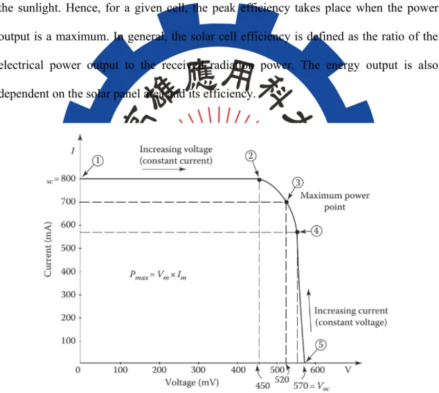
The power of the solar cell is a function of the cell area and the power density of the sunlight. Hence, for a given cell, the peak efficiency takes place when the power output is a maximum. In general, the solar cell efficiency is defined as the ratio of the electrical power output to the received radiation power. The energy output is also dependent on the solar panel area and its efficiency.
Figure. 9 Typical I - V characteristic of a photovoltaic cell. (source: Turan Gönen, Electrical Machines with Matlab)
The I–V characteristic is based on the ideal assumption that the solar cell is operating under a bright noontime sun. In some case that the power density of the sunlight is alleviated, the output of the cell decreases accordingly due to the fact that it is just rising or setting. However, nowadays the efficiency of the solar panel has been increasing as well to tackle those issue with Maximum Power Point Tracking (MPPT) that allows the solar panel tracking optimal solar radiate and able to absorb optimally.
Given the surface PV Area (m²) A, solar panel efficiency yield r, and solar radiation on tilted panels H, the global formula to estimate the electricity generated in the output of a photovoltaic system is the total absorption solar radiation in the tilted panel as given by:
Gpv=A ∙ r ∙ H (9)
2.1.3 Load Demand Modeling
The modeling of load demand is assumed to be a Gaussian distribution and find the variance in each day. The Gauss distribution often named as the normal distribution is the most important distribution in statistics. Where the standard distribution form is given by: f
(
x ;μ , σ2)
= 1 σ√
2 π e −1 2 ( x−μ σ ) 2 (10)where the parameter µ is a location parameter, identical with the mean value, and the σ is the value of standard deviation. When µ value is 0 and σ value equal to 1, it is
extensions is adequate to apply this regular form because µ and σ might be considered as the shift and scale parameter respectively.
Central Limit Theorem explained in the last paragraph indicates that if we add a huge number of random variables together, their sum of the distribution roughly will be normal under specific conditions. The importance of this result comes from the fact that many random variables in real life can be expressed as the sum of a large number of random variables and, the Central Limit Theorem, we can argue that distribution of the variable sum should be normal.
To proceed in load variance modeling, first the hourly historical data will be fitted by curve fitting, then the value attain from the curve fitting will be used to model random number with the estimation of load variance.
2.2 Optimization Problem, Classical Numerical Methods, and Deterministic Approaches
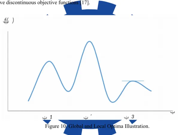
The optimization is involved in searching the optimal values of one or even some of problem-solving variables that appropriate with the objectives without violating constraints. Managing the optimization problems could have more than one, or even more result, and not all of them is global optima, it could have several local optima, however, it depends on the defined objective function. As an example, the graph in Figure 10 has an f(x) function which illustrates the objective possibly obtain the x value where the f(x) have its optimum value at xf(x). And obviously, the local maxima are all of the value x1, x2, and x3 that we observe. There is something that alleviates the function f(x)≥ f (x ± ε), and ε → 0 when occurring just little enhance or decrease of x, in
first order shape f(x) equal to 0 is feasible. Nevertheless, the objective function resulting local optima (x1 and x3) in the highest overall value for the global optimum x2. However, the frequently is difficult to specify as the global optimum or only local optimum, unlike this simple example, because of the complexity of solution space. The resulted variable will contribute from all of the objective functions which become considered part, then the problem space will become multidimensional which usually have discontinuous objective functions [17].
Figure 10. Global and Local Optima Illustration.
Classical numerical methods commonly derived from algorithms which have an iterative search that iteratively improve the initial guess of the solution according to the deterministic rule. As an example to applied the deterministic with Mathematical Programming methods which can manage the objective is in the financial optimization problem, the method also considers constraints contain both equalities and inequalities.
Next following paragraph will give some kind of method that suitable to implement in the kind of matter.
Dynamic Programming is likely a very common concept than an appropriate algorithm. The dynamic programming can be implemented to problems with the temporal structure. As an example in financial multi-temporal problems, the concept is to separate the problem in some areas as a subproblem. Initially, the last “A” sub of the problem should be obtained in the beginning, then the A – 1 is considered the final optimal solution, once the “A” solution found, the work proceed to find a solution in all sub of that problem.
To solve a problem which is a linear optimization, and the objective function have constraints both equality(is) or inequality(is), the Linear Programming would be suitable to solve the problem. Linear Programming is a basic problem solver that used in the various field such as engineering, economy management. In standard linear programming commonly the data are treated as certain or could be random parameters. The Simplex Method is the most common method use to apply where adding a slack variable in order to transform the inequalities become equalities and next searching solution from initial guess until the optimum obtained. This method works quite efficiently for many optimization problems, although this computational complexity is exponential. To came up the random parameters which are uncertain we can apply statistical analysis. The uncertain data parameters should incorporate into the model in some of the situation.
Mixed integer programming problems are established as those where several or all of the decision variables are only allowed to be integers. This is typically required in a range of real-world applications in allocation and planning problems where the discrete variables represent quantities, such as the number of individual shares to be held or the number of pipelines need or the number of electricity generator should be install, and all of those numbers is require integer values for the solution.
There a lot of optimization problems in scientific and engineering applications involve both nonlinear system dynamics and discrete decisions that affect the result of optimization problems. Mixed-integer nonlinear programming is one of the most general modeling examples in optimization, including both nonlinear programming (NLP) and mixed-integer linear programming (MILP) as sub-problems.
Mixed-integer nonlinear programming problems incorporate the combinatorial difficulty of optimizing over discrete variable sets with the challenges of handling nonlinear functions. Then it is well-known that MINLP problems are NP-hard because they are the generalization of MILP problems, which are NP-hard themselves. The most basic form of an MINLP problem when represented in algebraic form is as follows:
min z=f (x , y ) (11)
Subject to:
g(x , y)≤ 0 (12)
The Quadratic Programming can be implemented when the both of constraints equalities and inequalities are linear, and have quadratic form equation to solve the problem. This method basically same with Simplex Method, however, it is capable of solving the exponential case.
When we have an optimization problem that uses uncertain data to cooperate with an objective function, some of the Stochastic Methods can be applied. Statistical or numerical approaches with the estimation of some probabilities are assessed.
Another example with mathematical programming are integer programming, non-linear programming, binary programming, many kinds of algorithms to obtain optimum solutions. To conduct the optimization modeling, the structure model for the method is considered with the specific problem, as an example in mechanical optimization usually have a strict boundary and specific number which should not exceed the constraints to make decision variables.
The classical optimization method is separated in two categories. The first methods category based on full search or complete registration, for instance, checking every candidate solution. The main method such as branching and bounding will converge as much of feasible area as possible and eliminate candidates which already decide as bad initially. However, after eliminating some of the feasible solutions, candidates number left could yet outpace capacity, organize the solutions quantity is different and the first place is finite. Another classical optimization method type included are particularly derived from differential calculus, in this case, would use the
first order method and change the independent variables become a number with the derivative or objective function probably have 0 points.
The complete presumption is that there is only one best solution, possibly that best might be obtained on initial guess direct way. Optimization progress is generally derived from numerical deterministic rules. The interpret that given the similar initial guess values, iterated perform shall constantly result in similar output which is a dispute as unnecessarily fine result, iteration proceeds with same deterministically produced initial guess values would have similar results, and it is incapable to assess the result is the global optima or only local optima which is has been obtained. To demonstrate this deterministic method, it is illustrated in the function in Figure 10. If the initial guess for that x value is close to the x1 (local optima) or local optima in x3, however, the classical numerical procedure is potential to find in the local maximum which is closest with the initial guess, then the global optima x2 would be still difficult to discovered.
Practically the deterministic method behavior also the directly search for nearest value global optimum from the existing objective problem would become an important issue, for specific example when having a lot of local optima, and those of local optima is far away from the global optimum, however near with the initial guess or starting guess value. The minor enhancements of the objective function could result with immense values different from the decision variables.
The other common option to solve the deterministic problem should be Monte Carlo (MC) search. An extensively huge random number and appropriate with consider
then they consider the related variables of the objective function. With a quite big number of independent variable guesses, the approach like this possible to consequently identify the optimum value or at least to found the regions which are a possibility or impossible to be obtained. This method is more suitable compare than the classical numerical methods as its main limitation are a priori the availability of a suitable random number generator and the time necessary to carry an adequately huge range of attempt. Therefore, it could be applied to reduce the search space which can later be approached with classical numerical methods. This would become the main drawback of it, however, that it could be quite inefficient and inaccurate. Sometimes, it is quite often the important section of the opportunity set may shortly be identified far away from the real optimum value. Further search in this area is just time-consuming.
Heuristic optimization techniques and heuristic search methods also combine the stochastic elements. Unlike the Monte Carlo search, they have a procedure to guide the search towards the feasible area in the opportunity region. Therefore, they integrate the advantages from the previously presented approaches. Then just similar with the numerical methods, they set to converge to the optimum in the method of iteration search, however, they are possibly less to obtain the local optimum and global optimum, they are highly flexible and therefore are less limited or might be absolutely unrestricted to certain forms of constraints.
The heuristics discussed in a proper way and implement in the primary section of the object function was designed to solve optimization problems by again and again generating and examine new solutions. These optimization techniques, therefore, guide problems where there really be found by a well-defined model and objective function.
2.3 Heuristic Optimization
Generally, the main characteristic of heuristic optimization methods is the method begin with an initial solution which has extra or less changeable, then yields new optimal solutions iteratively from a specific range of generation then select these solutions and these new solutions would be evaluate, finally will resulting the optimum solution generated during the optimization progress. The process of the iteration procedure is usually stopped when there is no further improvement after the given number of generations (or the result enhancements cannot be evidence), when the optimal solution found is quite good, and when already reached the computational time limit has, or even when several of parameter halt the process. The next evidence of stopping criterion for right result value could be a burden the computational progress. Since heuristic optimization methods possibly to be different enormously in every specific approach, to obtain such a common diversification scenario is hard. The explanation below is considered several major aspects that afford to compare between some of the approaches.
1. New Solutions Generation
The new solutions able to produce by modifying the solution before or even by construct new solutions based on last results. The random guess of the deterministic rule or might combination from both of them (e.g., deterministically produce alternative variable and randomly select one of them) can be implemented.
To deal with local optima, the heuristic method usually considers not just for those latest lead solutions to an enhancement directly, the new solution also treats some of those inferior solutions together along with the best solution found. In order to increase convergence speed, the worst produced solutions could also either be included in a condition not extremely different with the optimum. In the other hand, the too high best solution might be increased, the new produces solutions could be graded and keep the best for next decision. The obtained regulation can be deterministic or have specific random order.
3. Search Agents Number.
Although in some of the heuristic methods, the single agent pointed to update the solution, generation based approaches usually make the use of collective result accumulate in previous iterations.
4. Limit of Feasible Area Bound
Having the enormous population area, the new groups of solutions could be obtaining by search inside a specific near from the current search agent. Some other methods explicit remove some of the neighborhoods areas to keep away the cyclical search pathways or expend substantial calculation time on inconsequential option.
5. Prior Knowledge.
When have a common rule of what is good objective would possibility to implement in such as problem, the prior of knowledge could be implemented in the option of initial guess solutions within the optimization work as the guided search. Although with the participation of prior knowledge would significantly narrow the
feasible area in the search space and speed up the convergence, this would possibly cause guided to the bad solution results as the optimization take the wrong objective or the algorithm might occur difficult to find global optima and local optima. Therefore, the prior knowledge is set up in a rather than bounded the value of heuristic optimization approach rather than a precondition.
6. Specific Constraints Flexibility.
Though there is have common objective approaches which able implemented into exact any variants of optimization area, some of the approaches are called “tailor-made” which is mean as the approaches is a specific variant of constraints. Therefore, it would be inappropriate to fit the designated approach with other optimization problem works.
In the heuristic method, some of them are inspired by nature as the evolution based on genetic methods, the ideas of implemented the evolution theory and artificial life attain some of the methods in computational intelligence. In the heuristic optimization method, the algorithms which subject to the optimization problem are called well known “Evolutionary Algorithm”. The initial solution of P population vectors is generated at the beginning. Each the generation process, every individual genome is treated as a parent that will generate offspring with involving random alteration to the parent’s solution. After that, the population multiplied and only the finest parameters agents picked then will maintain the population in the next iterations.
chromosomes “X” which represents fitness value in the population. To find the fittest solution output, the superior fitness escalates the multiple reproduction opportunities, the low fitness value obviously would lead to elimination. The new population offspring is produced from two chromosomes combination. Moreover, the mutation operators able to take over generated population by randomly modifying the existing solution. More than decades, the Genetic Algorithm become the excellent method in the evolutionary algorithm optimization, because of the value of crossover operator’s options, mutation rate, and cloning of the existing chromosomes.
2.3.1 Genetic Algorithm
The Genetic Algorithm is categorized as a stochastic global search method which copies the theory of biological evolution. Genetic Algorithm performs on a potential solutions population by implementing the survival of the fittest rule to generate better estimation to a solution. In every generation, the latest approximations set is produced by the works of selecting individuals correspond to their fitness value in the problem area and reproducing them together using operators setting as natural genetics. Because of this, the evolution of individual in populations are better suited to their environment than the individuals that they were created from.
As those characteristic, it can be observed that the Genetic Algorithm very different with others classical optimization and search approaches. The major significant differences are:
• Derivative information or another auxiliary knowledge is not necessary for Genetic Algorithm, the directions of search influence only by the objective function and corresponding fitness levels.
• Genetic Algorithm does not use deterministic, rather than use stochastic transition rules.
• Genetic Algorithm able to work on an encoding of the parameter set rather, except when
using real-valued variables.
As to remember Genetic Algorithm give a potential solutions value to a specified optimization problem and the final decision depends on the user. In cases where a specific optimization does not have one individual solution, for example, Pareto-optimal solutions, multi objective optimization and scheduling problems, the Genetic Algorithm is potentially helpful to find these solutions options in the same times. The main factor in the Genetic Algorithm process is described below:
1. Population Representation and Initialization
A number of potential solutions that proceeds on Genetic Algorithm are named a population, composed by several encoding of the variable set together. A population usually is consisting of between 30 to 100 individuals. however, in some variant of the problem will have different implementation, there is a variant named the micro Genetic Algorithm to apply an extremely small number of populations, which have 10
individuals with a restrictive implementation of reproduction and replacement strategy, as an effort to reach real-time execution.
While binary encode chromosome type is the most commonly used in Genetic Algorithm, the alternative encoding technique also increasing concern, for example, the real-valued and integer representations. In several problem cases, the binary representation is disputed is unreliable as blind the searching nature. For example, in the subsection selection problem, the utilization of an integer value representation and look-up tables give a convenient and natural way of expressing the mapping from representation to problem domain.
The Genetic Algorithm with real value phenotype use is stated offer a numerous of benefit in numerical function optimization than binary representations. the Genetic Algorithm efficiency is boosted up because there is no need to convert phenotypes before every evaluation function, therefore, just small amount of memory is required due the efficient of floating-point internal computer representations can be used directly. The precision by discretization to binary or other values also do not have lost, moreover, it gives an extra free approach to implement in the different genetic operators.
2. Selection
The process to determine the times value or trials is called Selection, a certain individual is select for generating offspring. The individual’s selection can be assumed as 2 distinct processes. First, the determination of the trials amount, an individual can expect to accept. second, the alteration of the expected number of trials into a discrete number of offspring.
3. Crossover
The recombination process or called by Crossover is the Genetic Algorithm basic operator for producing new chromosomes. As the nature characteristic, the new individuals generates by crossover possess several sections from parent’s genetic character. The simplest form of crossover is that of single-point crossover, described in the Overview of GAs. In this Section, a number of variations on crossover are described and discussed and the relative merits of each reviewed.
2.3.2 Differential Evolution
Global optimization problem through continuous areas is often present in the whole of the scientific area. Generally, to optimize a specific characteristic of the system with choosing parameters in the system. To simply and ease, a parameters system generally described as a vector.
The basic approach of the optimization problem is initiated by designing the objective function that could exhibit the objectives problem include with constraint limitations. Mostly the objective function defines the optimization problem as a minimization task. In those example problems, the objective function is precisely considered as a cost function. If the function is nonlinear and non-differentiable, direct search methods are the choice.
After the random variable generated, the decision must be made whether appropriate with derived parameter or not. Most of the standard direct search approach
criterion, all of the latest parameter vectors is feasible if it reduces the value of the cost function. Even though the greedy search works converges quite fast, it has the risk fell in a local minimum. Executing some vectors simultaneously, better parameter settings could help other vectors avoid local minima. Generally, people need the practical minimization method to fulfill four requirements:
(1) Able to handle linear, nonlinear, differentiable, non-differentiable, and multimodal cost functions.
(2) Parallel ability to solve computation with intensive cost functions.
(3) Simple and Ease to use, for example, less organize variables to adjust the optimization. These Variables would also be robust and easy to select.
(4) Well convergence characteristic, for example, consistent convergence to the global minimum in continues stand-alone test.
Having some of the requirements mentioned above, the Differential Evolution was designed to be a stochastic direct search method to meet the first requirement. Utilize with direct search technique have the benefit of being simply implemented to optimization experiment where the cost value is derived from a physical test rather than a computer simulation.
The second requirement is necessary for demanding computational optimizations, as an instance, the optimal function evaluation may obtain from time variants (hours to days), and it is often implemented in finite element simulation or integrated circuit design. in order to achieve feasible results in an appropriate time consumes, the only reasonable way is to apply a parallel computer. Differential
Evolution meet those demand by implement stochastic variable in a vector population which able to complete independently.
To complete the third requirement, if the optimization method is automatically arranged it will be advantages because only little input is required from the user. The new variable vectors are generated by considering highest variables and shorten around the low variable. The new variable will substitute their old variables if they fit with the function value with reduced cost compared to their previous. These methods allow the search space, i.e. the polyhedron, to expand and contract without special control variable settings by the user.
The last requirement number 4 needs good convergence characteristic, there are mandatory for a well construct optimization algorithm. Although plenty methods found is theoretically express the convergence characteristic of a global minimization method, just comprehensive attempt within several conditions may exhibit whether a minimization approach can meet the requirement.
As a parallel direct search approach, the Differential Evolution starts with a number of population (NP) candidate solutions, which may be represented as
xi, G ,i=1,2,. . . , NP (14)
where i index denotes the population and G denotes the generation to which the population belongs. The Differential Evolution process depends on the manipulation
In the population for every generation G. NP does not change during the optimization work. The initial variable population is randomly chosen and should cover the entire variable space. Normally, an identical probability distribution for all random variable except the stated variable. If the preliminary solution is available, the first population could be produced by increase the normal distributed random variation to the nominal solution xnom,0. Differential Evolution results in latest variable vectors by including the weighted difference between two population vectors to a third vector. This operation is called by mutation.
Next is the variable mixing is referred by crossover. The mutated variables vector mixed with the variables in the another decisive vector, the target vector, to yield the so-called trial vector.
The last operation is selection, when the test vector results in a lower cost function value than the objective vector, the test vector replaces the objective vector in the next generation. Each population vector has to provide once as the objective vector so that NP tournament occurred in one generation. Next following paragraph explains Differential Evolution’s basic strategy specifically:
1. Mutation
As the main operator of Differential Evolution, the execution of this process causes Differential Evolution dissimilar from other Evolutionary algorithms. The Differential Evolution mutation process uses the vector differentials between the current population variable for specifying both the value and way of perturbation used to the individual subject of the mutation process. The mutation process at each generation
begins by randomly selecting three individuals in the population. For each target vector xi ,G ,i=1,2,. . . , NP , a mutant vector is generated according to
xi ,G +1=xr 1 ,G+F .(xr 2 ,G−xr 3 ,G) (15)
with random indexes r 1, r 2 , r3 ∈ {1, 2, . . . , NP}, integer, mutually different and F > 0. The randomly chosen integers r 1, r 2 , r3 are also chosen to be different from the running index i, so that NP must be greater or equal to four to allow for this condition. F is a real and constant factor ∈ [0, 2] which controls the amplification of the differential variation (xr 2,G−xr 3, G) .
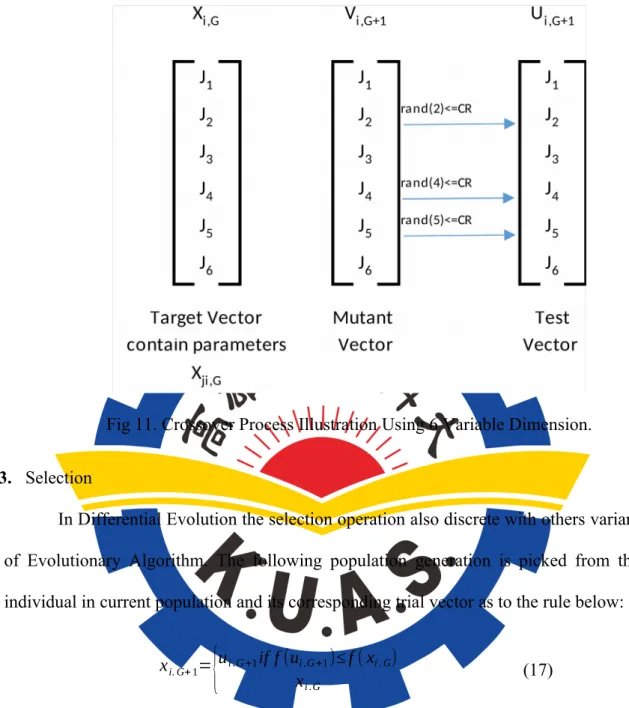
2. Crossover
After the mutation process done, next proceed to the crossover operation. The perturbed individual, vi , G+1=(v1 i , G+1+v2i , G+1, .. . , v¿,G +1) , and the previous population
member xi ,G +1=(x1 i ,G +1+x2 i , G+1, .. . , x¿,G +1) ,are subject to the crossover operation,
that finally generates the population of candidates, or “trial” vectors
ui ,G+1=(u1 i ,G +1+u2 i ,G +1, . . ., u¿,G +1)
uj , i .G +1=
{
vj ,i .G +1if randj≤Cr⩗ j=kxj ,i . G+1
(16)
Where, j = 1. . . n, k ∈ {1, . . ., n} is a random parameter’s index, chosen once for each i, and the crossover rate, Cr ∈ [0, 1], the other control parameter of Differential Evolution, is set by the user. Figure 11 below showed example of crossover process in 6 dimension vectors.
Fig 11. Crossover Process Illustration Using 6 Variable Dimension.
3. Selection
In Differential Evolution the selection operation also discrete with others variant of Evolutionary Algorithm. The following population generation is picked from the individual in current population and its corresponding trial vector as to the rule below:
xi. G+ 1=
{
ui .G+1if f (ui .G+1)≤ f ( xi . G) xi .G(17)
Thus, every individual in the test population appealed with their counterpart in the current population. Lowest individual objective function value will survive from the competition selection to the population in the next generation. As a result, all the individuals of the next generation are as good or better than their counterparts in the current generation. In Differential Evolution the test vector is not compared against all
the individuals in the current generation, but only against one individual, its counterpart, in the current generation.
CHAPTER 3 PROPOSED APPROACH
3.1 Model Description
The objective in this proposed approach is to implement the renewable energy and hybrid system into smart grid management. With the randomness of the wind and solar, the grid system should able to cover all of the load demand with the help of storage system. The wind and solar generated output matrices will match with load variance matrices to find the efficient component sizing should be installed [6]. The difference value from power generation load demand will consider the storage system should supply the load demand or charging. When the generation power exceeds more power, the surplus energy will manage to store in the storage system. However, when the generating power needs extra energy the storage system will support to supply load demand.
Figure 12. Hybrid Renewable System in Smart Grid Interconnection.
The considering the load demand should be helpful to avoid the peak average rate and maintain the power system in balance, the distribution of load demand also takes into account for this simulation as the load demand management in power scheduling method. In this approach, that load distribution will represent as the load shifting. The flexibility and the effectivity of the storage system will also have determined by the rate of load shifting and the charging/discharging storage.
Using Evolutionary Algorithm such as Genetic Algorithm or Differential Evolution would be suitable to attain the optimal capacity of installed wind energy source, solar energy source, and storage system capacity. Initially, the huge population will be constrained, selected from the feasible area and evaluated by the fitness function, then the crossover and mutation function will proceed to achieve the optimal solution.
The randomness of renewable energy such as wind and solar would be difficult for the evolutionary algorithm to find the optimal solution. The Evolutionary Algorithm will face to the huge computational burden for the uncertain result and will be difficult to converge to global optima. To minimize that computational burden, we need to perform some statistical methods or simulation to achieve the point estimation from the uncertain model then the optimal solution of renewable energy able to solve with evolutionary algorithm [9]. The details of proposed approach illustrated in the flowchart below and will explain in the next paragraph.
Figure 13. Flowchart Proposed Optimization Method in GA.
First of all, the input data historical solar irradiance, wind speed, and load demand are used to find the probability model which is represent the nature of wind
No Yes No Max Gen Storage Charging Storage Discharging
Calculate ES, Load Shifting, Sc
S>Smin Input Data (wind, solar, load)
Fit Data Distribution Probability Function
ES > 0
Set Power Estimation Point with MCS
Initialize Population
Increase Lst Yes
Evaluating Fitness Function, Constraints and calc max(Sc) Penalty Factor
Crossover and Mutation
No
Yes
Calculate Power with PDF setting
speed, solar irradiance, and load demand [13]. Using curve fitting we can obtain the probability model of the nature source that will we use to determine the component sizing for each scale of the wind and solar generating power. For the load demand, the normal distribution or Gaussian distribution is applied to model lower bound and upper bound of load variance. Having the parameters from the curve fitting we can generate the pseudo random number with the probability function. Those random number generated will reassemble the nature data that fitted in curve fitting.
Wind Speed Data (mph)
Figure 14. Fitting Wind Distribution.
With Weibull distribution the wind distribution fitting will obtain parameters as follow:
Mean: 5.02301
Variance: 11.0614
Parameter Estimate Std. Err.
α 5.5816 0.7782
β 1.54152 0.250919
Estimated covariance of parameter estimates:
A B
A 0.605595 0.0611139
B 0.0611139 0.0629604
Solar Radiation (KW)
Figure 15. Fitting Solar Distribution.
Log likelihood: -165.429
Domain: 0 < y < Inf
Mean: 362.564
Parameter Estimate Std. Err.
α 1.03324 0.263384
β 350.9 113.87
Estimated covariance of parameter estimates:
a b
a 0.0693711 -23.5592
b -23.5592 12966.4
Load Demand (MW)
Figure 16. Fitting Load Distribution.
Log likelihood: -236.221
Domain: -Inf < y < Inf