An Efficient Perfect Algorithm for Memory Repair Problems
Hung-Yau Lin
1, Fu-Min Yeh
2, Ing-Yi Chen
3, and Sy-Yen Kuo
41, 4
Department of Electrical Engineering, National Taiwan University, Taipei, Taiwan.
2Chung-Shan Institute of Science and Technology, Taoyuan, Taiwan.
3
Department of Computer Science and Information Engineering, National Taipei
University of Technology, Taipei, Taiwan.
1
hylin@lion.ee.ntu.edu.tw
2fmyeh@tpts5.seed.net.tw
4sykuo@cc.ee.ntu.edu.tw
Abstract
Memory repair by using spare rows/columns to replace faulty rows/columns has been proved to be NP-complete. Traditional perfect algorithms are comparison-based exhaustive search algorithms and are not efficient enough for complex problems. To overcome the deficiency of performance, a new algorithm has been devised and presented in this paper. The algorithm transforms a memory repair problem into Boolean function operations. By using BDD (Binary Decision Diagram) to manipulate Boolean functions, a repair function which encodes all repair solutions of a memory repair problem can be constructed. The optimal solution, if it exists, can be found efficiently by traversing the BDD of a repair function only once. The algorithm is very efficient due to the fact that BDD can remove redundant nodes, combine isomorphic subgraphs together, and have very compact representations of Boolean functions if a good variable ordering is chosen. The remarkable performance of the algorithm can be demonstrated by experimental results. Because a memory repair problem can be modeled as a bipartite graph, the algorithm may be useful for researchers in other fields such as graph theory.
1. Introduction
The density of memory chips increases constantly along with the advancement of VLSI technology. As the chip density increases, it becomes harder and harder to manufacture chips that contain no defect (or faulty cell). In volume semiconductor manufacturing, an increase in yield of a few percentage points can have a substantial impact on the profit. For chips that have a uniform structure such as Random Access Memory (RAM), one of the techniques to improve the yield is to use spare rows and columns to replace faulty rows and columns. These devices are referred to as Redundant RAM (RRAM). It has been proved that memory repair by using row/column deletion is NP-complete [1]. A lot of heuristic approximation algorithms have been proposed to speed up the process [1-9] but only a few perfect algorithms have been presented [1-2, 10]. An algorithm is called a perfect algorithm if it can find a repair solution whenever a solution exists. Though heuristic algorithms are very efficient, they have a common drawback: they cannot guarantee a solution to be found even if one solution exists. Perfect algorithms seem to be more preferable but they are not efficient enough for complex problems.
The exhaustive search used in traditional algorithms consists of the following steps. A faulty cell is chosen and it is repaired with a spare line. A line is a row or column. This step branches into two subproblems since the faulty cell can be repaired with a spare row or a spare column. These two subproblems are inserted into a queue. The queue is sorted according to some use-defined cost functions and duplicate records (or partial solutions)
are removed from the queue. The first record in the queue is chosen and removed from the queue. If this partial solution contains no faulty cell, it is the repair solution. Otherwise, it is branched into two subproblems which are also inserted into the queue. Repeat this process until a solution is found or no solution can be found. This algorithm is known as the branch-and-bound (B&B) algorithm [1] or fault-driven approaches in other literatures.
Improvements to exhaustive search algorithms are proposed in [2, 10]. Instead of choosing randomly a faulty cell for branching, they choose the line that contains the most number of faulty cells and repair the line with a spare line of the same type (row or column) or many other spare lines of the other type. They also use an initial screening algorithm to screen out single faulty cells. A single faulty cell is a faulty cell that does not share its line with any other faulty cells. A branch-and-bound algorithm incorporating these improvements is called an improved B&B (IB&B) algorithm in this paper.
Even with these improvements, traditional algorithms such as IB&B are not efficient enough for complex problems. One of the reasons is that they are in essence comparison-based exhaustive search algorithms. It takes time to copy data from a parent partial solution to two subproblems. It takes more time to sort the huge number of records and make these records unique in the queue. This time consuming computation is needed to process a single partial solution at the head of the queue. As the problem becomes more complex, more data in each record needs to be compared. Even worse, much more records will be inserted into the queue because of the exponential growth rate of branching operations. Imagine that there are thousands of records in the queue and the drawback of comparison-based exhaustive search algorithms becomes evident.
Instead of trying to improve the performance of traditional algorithms as other researchers have done, a new algorithm has been devised and presented in this paper. The algorithm transforms a memory repair problem into Boolean function operations. A repair function encoding all repair solutions can be constructed by using BDD (Binary Decision Diagram) [11-12] to manipulate those Boolean functions. It can be proved that a repair function does encode all repair solutions. By traversing the BDD of a repair function only once, a repair solution can be quickly found if it exists. Besides, finding an optimal repair solution is as easy as finding a non-optimal one. An optimal repair solution is defined to be the solution that contains the least number of spares. The algorithm is very efficient due to the fact that BDD can remove redundant nodes, combine isomorphic subgraphs, and have very compact representations of Boolean functions if a good variable ordering is chosen. The remarkable performance of the algorithm can be demonstrated by experimental results. Unlike other exhaustive search algorithms which stop searching when a repair solution is found, the algorithm encodes all solutions in the repair function. This may be of use in some applications. Since a memory repair problem can be modeled as a bipartite graph, the algorithm may be of use for researchers in other fields such as graph theory.
2. The BDD-based algorithm
Not much improvement to the traditional perfect algorithms has been made in recent years. One possible reason is that making great improvement is difficult and heuristic algorithms are used because of the high complexity of perfect algorithms. Instead of trying to improve traditional perfect algorithms, a new algorithm is devised. The algorithm avoids the huge number of copy and comparison operations inherent in traditional algorithms by transforming a memory repair problem into Boolean function operations. The algorithm uses BDD to perform the underlying Boolean function operations. The BDD-based algorithm BDDRepair is shown in Table 1. BDD, DF, CF, and RF will be described in detail in the following sections.
2.1. The defect function DF
A defect function is a Boolean function which encodes the lines (or locations) in which faulty cells should be repaired. If Ri and Ci are used to denote the row and column variables of a faulty
cell i, it is obvious that the following defect function DF will encode all faulty cells of a memory repair problem:
(
)
∏
+ = i cell faulty each for i i C R DF _ _ _ _ (1)A faulty cell can be repaired by using a spare line and this corresponds to the term Ri+Ci in
the parentheses. In order to repair all faulty cells, the terms inside each parentheses pair need to be true. More than one faulty cell may appear in the same row, say Ra. In this case, many terms
in equation (1) will contain Ra. If Ra is true, the terms containing Ra will be evaluated to true. This means that a spare row can repair many faulty cells in the faulty row Ra.
2.2. The constraint function CF
One of the obstacles of developing the BDDRepair algorithm is the construction of a constraint function. A constraint function is a Boolean function encoding all combinations of faulty lines that spare lines can repair. If a memory array has s spare rows and d defect rows (faulty rows), the constraint function for row CFr can be built with the following function:
∑
= = = i s i d i r C CF 0 (2)The meaning of this constraint function is simple and intuitive. Among the d faulty rows, i faulty rows can be repaired and i can range from zero and up to s. If i is less than d, it means i spare rows are used and all other faulty cells not repaired by i spare rows should be repaired by spare columns. Each combinatorial function represents a valid combination of spare rows.
It is not practical to enumerate all terms of the combinatorial functions and a better solution has to be devised. Assume the symbols of those d faulty lines are put into an array L and use L0, L1, ..., and Ld-1 to denote the symbols in L. A placement function PF can be defined as follows:
PF
(
Lk,d,s)
=Lk•PF(
Lk+1,d−1,s)
+Lk•PF(
Lk+1,d−1,s−1)
(3)The meaning of equation (3) is easier understood with the following description. If a faulty line
Table 1. The BDD-based algorithm BDDRepair.
BDDRepair() {
Choose a variable ordering using a heuristic algorithm; Construct the BDD of the defect function DF;
Construct the BDD of the constraint function CF;
Construct the repair function RF by using the equation RF = DF AND CF; Traverse RF;
if (RF contains only one BDD node bdd_zero) no repair solution can be found;
else
report a repair solution; }
Lk is to be repaired by a spare line, the number of spare lines will be one less than the original. If Lk is not to be repaired by a spare line, the number of spare lines will remain the same. In both
cases, Lk is removed from the set of faulty lines and the number of faulty lines left will be one less than the original. The performance of equation (3) can be improved by using a hash table to avoid redundant computation. The CFr can then be constructed with equation (4). Equation (4) can be proved by mathematical induction and the proof is skipped in this paper.
( 0, , ) 0 s d L PF C CF s i i d i r =
∑
= = = (4) Equation (5) and (6) shows two useful properties of the placement function. These two properties are intuitive. If the number of spare lines is greater than the number of defect lines, all defect lines can be repaired and true is returned. If there is no spare line left, then none of the defect lines can be repaired and the symbols of these defect lines need to be complemented and ANDed together.PF
(
Lk,d,s)
=true if d≤s. (5)PF
(
Lk,d,0)
=Lk•Lk+1•Lk+2•L•Lk+d−1 (6)The constraint function for column CFc can be constructed in the same way as CFr. Then, the final constraint function CF can be constructed with the following equation:
CF = CFrAND CFc. (7)
2.3. The repair function RF
The repair function is a Boolean function that encodes all repair solutions of a memory repair problem. Since the defect function encodes the lines to be repaired and the constraint function encodes the lines that spare lines can repair, it is obvious that the repair function can be constructed with equation (8). Section 3 will prove that a RF does encode all repair solutions.
RF = DF AND CF (8)
After a RF has been built, a repair solution can be found by traversing the BDD of a RF only once. A path from the top variable to the terminal node bdd_one is called a solution path. All variables in a solution path taking the 1-edge form a repair solution. The 1-edge or 0-edge in a BDD can be represented by pointers in some computer languages. By following pointers, a repair function can be traversed efficiently.
2.4. A simple example
A very simple problem as shown in the left of Figure 1 is used as an example to illustrate the
algorithm BDDRepair. Because the BDD of CF, DF, or RF can have thousands of nodes for complex problems, it is impossible to draw in this paper a BDD with plenty of nodes. Note this example can be repaired by the initial must-repair screening algorithm [1-2]. It is used because of its simplicity since the initial screening algorithm can be incorporated into our BDD-based algorithm with easy. The 3x3 memory array has one spare row (SR) and one spare column (SC). The darkened cells are faulty cells and others are normal cells.
The first step is to choose a variable ordering and assume the variable ordering (R1 < C1 < C3 < R3) is chosen. Then, the defect function is built by using equation (1):
DF = (R1+C1)(R1+C3)(R3+C3)
The BDD of this defect function is shown in Figure 1. Before the constraint function can be built, the CFr and CFc have to be constructed by using equation (4), (5), and (6). There are two faulty rows in the memory array and assume R1 and R3 are inserted into the array position 0 and 1 respectively. Then CFr can be built as shown next.
3 1 1 1 0 0 1 0 0 1 0 1 0 0 1 0 2 PF(L,21,) L PF(L 1,1,) L PF(L,,10) L true L L L L L R RR C CF i i i r =
∑
= = • + • = • + • = + = + = =Similarly, CFc can be built in the same way. The constraint function can now be built with equation (7) as shown below and the BDD of this constraint function is shown in Figure 1.
3 1 3 1 1 3 1 3 1 1 1 1C RCC RRC RRCC R CF CF CF= r• c= + + +
Finally, the repair function can be constructed by using equation (8) and its BDD is shown in Figure 1. There is only one solution path in Figure 1 and it is
(
R1C1C3R3)
. Therefore, the repair solution to this example problem is R1C3. Please note that the Boolean equations above are shown only for illustration. BDD representations are constructed and used in our algorithm.3. Mathematical proof
This section proves that the repair function does encode all repair solutions of a memory repair problem. Assume there are SR spare rows, SC spare columns, and f faulty cells in a memory. The faulty cells are
(
Ri1,Ci1)
,L,(
Rif,Cif)
. Also assume that these faultycells scatter in FR rows and FC columns, that is, there are FR faulty rows and FC faulty columns. Note that some of the faulty cells may lie in the same line. Thus, f is not necessarily equal to FR or FC.
The next equation shows the defect function.
(
Ri Ci)(
Ri Ci)
(
Rif Cif)
DF = 1+ 1 2+ 2 L +
This equation can be expanded by picking m terms from the row variables and f −m terms from the column variables. For example, if m equals to 1, any one of the row variables can be picked. Though there are m product terms of the form
(
Rx1Cx2Cx3LCxf)
andthey have to be summed up together, only one general term is used to represent this notion. A new subscript x is used instead of the original subscript i to emphasize that Rx can map to any of the row variables Ri. Now the defect function can be rewritten as:
(
)
(
)
∑
− = = • • • • • • = 1 + + 1 ] [ 1 2 ( 1) ( 2) f k k x x xk xk xk xf C C C R R R DF L L[
] [
FC]
SC FC FC FR SR FR FR SC n n FC n SR m m FR m c r CF C C C C C C C C CF CF = + + + • + + + • = • =∑
∑
= = = =0 0 0 1 L 0 1 LNote that it is assumed that SR ≤FR and SC ≤FC. If SR >FR or SC >FC, the corresponding term in the square brackets will be true which means that all faulty lines can be repaired by the spare lines. One of the combinatorial functions, say CFR
1 , is used as an example for expansion. FR
C1 means that one of the faulty lines can be picked from FR faulty lines for repair. C1FR can be
expanded into many terms and these terms have to be summed up together. A general form
(
Rq1Rq2Rq3LRqFR)
is used to represent these terms inFR
C1 . By using such generalized terms, the
constraint function can be rewritten as:
(
) (
)
(
)
(
) (
)
(
)
] [ ] [ ) 1 ( 1 2 1 2 1 ) 1 ( 1 2 1 2 1 FC SC SC FC FC FR SR SR FR FR u u u u t t t s s s r r r r q q q p p p C C C C C C C C C C R R R R R R R R R R CF L L L L L L L L L L + + + + + • + + + =The equation above can be expanded by taking one term in each of the square brackets pair. For example,
(
)
FR
q q q R R
R1 2L and
(
Ct1Ct2LCtFC)
can be taken from each side of themultiplication sign and this creates the product
(
)
FC
FR t t t
q q
q R R C C C
R1 2L 1 2L . There are many terms of this form after expansion because the generalized term
(
)
FR
q q q R R
R1 2L is used in the previous step. Therefore, a generalized term for this product shall also be used and the
product can be rewritten as
(
)
FC FR w w w w w v v v v v vR R R R R C C C C C
R1 2L α (α+1) (α+2)L 1L β (β+1) (β+2)L . Note that the
notation
(
)
FR v v v v vR R R R R1 2L α (α+1)L can represent(
)
FR v v vR RR1 2L if α equals to zero. The
constraint function can then be rewritten with these generalized terms.
Finally, the RF can be obtained by multiplying (Boolean ANDing) DF and CF. By using the techniques similar to those presented above, the multiplication can be expanded into the following form.
(
)
(
)
[
]
[
(
)(
)
]
(
)(
)
[
]
∑
∑
∑
+ + + + + + + + = • • • • • • • = • = = = = = = = FC f k k FR k FC FR f k k k w w w w x x x v v v v v x x x SC SR w w w w v v v v v f k k x x x x x x C C C C C C C R R R R R R R R C C C C R R R R R C C C R R R CF DF RF L L L L L L L L L L L L ) 1 ( 1 ) 2 ( ) 1 ( ) 1 ( 2 1 2 1 ) 1 ( 1 ) 1 ( 2 1 ) 2 ( ) 1 ( 2 1 , 0 , 0 1 β β α α β β α α β α β αIt is well known that a Boolean variable R multiplied with its complement R is zero
(false). Note that
(
)
FR v v v v vR R R R
R1 2L α (α+1)L contains each faulty row variables and
(
Rx1Rx2LRxk)
denotes the row variables that should be repaired. Besides,
(
)
α
v v vR R
R1 2L represents the
rows that are to be repaired by spare rows and
(
)
FR
v
v R
R( +α1)L represents the rows that are not to be repaired by spare rows. If a row variable in
(
)
k
x x xR R
R1 2L is not contained in
(
Rv1Rv2LRvα)
, the row variable will be a member in(
Rv( +α1)LRvFR)
and the product term willbe false. In this case, that term in the square brackets will be false and it will not be a solution path. This means that the faulty rows (not necessarily all faulty rows) that must be repaired cannot be replaced by spare rows. If the term in the square brackets is not zero, it will be a solution path. In such case, any row variable in
(
)
FR
v
v R
R( +α1)L will not appear in
(
Rx1Rx2LRxk)
and each variable in(
Rx1Rx2LRxk)
will also be in(
Rv1Rv2LRvα)
. The same claimand can be eliminated from the summation part of the repair function, each term left in a RF will be a solution path. Thus, a RF encodes all solutions of a memory repair problem.
4. Experimental results
To evaluate the performance of our BDDRepair algorithm, we compare it with IB&B because IB&B is one of the most efficient perfect algorithms we know. The CMU BDD library developed by David E. Long was used to handle the required BDD operations [13]. All other programs were written in C++. Many C++ STL containers were used to speed up the development process. The hardware system contained a single Pentium III CPU running at 1 GHz with 512 MB of memory. The operating system was Linux 2.4.22. All program files were compiled with the compiler gcc 3.3.2 and the optimization flag -O2.
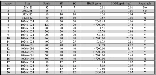
Many experiments have been conducted and Table 2 shows some of the results. The SR and SC are the number of spare rows and spare columns respectively. All spare lines are assumed to have no defect. The Faults in Table 2 denotes the number of faulty cells. All execution time are in CPU seconds. If there is only one node bdd_zero in a RF, then no solution can be found and the memory array cannot be repaired. The column Repairable indicates if a memory array is repairable or not. The arrays in Table 2 are randomly generated because real patterns (or distributions) of defects are not available for testing. Some arrays contain slightly clustered faults while others have sparse or scattered faults.
Most published data only list the number of faulty cells. But more faulty cells do not always imply longer execution time. The number of spare lines and the patterns of defects also have a great impact on execution time. Table 2 can demonstrate this statement. Arrays 17-20 have merely 50 faults and their execution time range from about 1 second to 40 minutes. Another example is Array 5 and Array 7. Thus, the execution time in previously published papers cannot be used directly. Different algorithms have to be implemented and the same test cases have to be used as input. To make objective judgments about performance, many experiments need to be conducted.
The experimental results indicate that BDDRepair significantly outperforms IB&B. This remarkable performance is achieved with the following advantages over traditional perfect algorithms. BDDRepair avoids the time consuming operations inherent in
Table 2. Performance comparison between IB&B and BDDRepair.
Array Size Faults SR SC IB&B (sec) BDDRepair (sec) Repairable
1 128x128 32 7 7 0.11 0.01 No 2 256x256 35 7 7 0.01 0.01 Yes 3 512x512 60 10 10 0.50 0.04 Y 4 512x512 60 10 10 0.57 0.03 N 5 1024x1024 60 20 20 2643.45 0.06 Y 6 1024x1024 120 20 20 > 7200.00 0.44 Y 7 1024x1024 200 20 20 4.51 0.93 Y 8 1024x1024 200 20 20 27.76 0.96 Y 9 1024x1024 200 20 20 530.65 0.93 Y 10 1024x1024 260 20 20 > 7200.00 20.78 Y 14 1024x1024 400 25 25 1936.73 0.51 Y 11 4096x4096 200 40 40 33.79 4.17 Y 12 4096x4096 400 40 40 > 7200.00 1.47 Y 13 4096x4096 500 40 40 > 7200.00 19.77 Y 15 4096x4096 500 40 40 > 7200.00 15.45 Y 16 4096x4096 500 40 40 > 7200.00 13.93 N 17 1024x1024 50 12 12 0.88 0.07 Y 18 1024x1024 50 12 12 3.03 0.07 Y 19 1024x1024 50 12 12 517.89 0.03 Y 20 1024x1024 50 12 12 2439.34 0.07 Y
traditional algorithms by transforming a memory repair problem into Boolean function operations. It uses highly efficient BDD algorithms to manipulate Boolean functions. BDD can remove redundant nodes, combine isomorphic subgraphs, and have very compact representations of Boolean functions if a good variable ordering is chosen.
However, BDDRepair does have a drawback. Like other BDD-based algorithms, the efficiency of BDDRepair highly depends on the variable ordering. A heuristic algorithm MaxRelated was used to find a variable ordering. The basic idea of MaxRelated ordering is to keep more related variables closer. Two variables are related if one variable depends on the other to determine the value of a Boolean function. MaxRelated algorithm seems to be able to find a relatively good variable ordering for most of the arrays we have tested but it does not guarantee to find one. If a bad variable ordering is used or no good variable ordering can be found for a problem, BDDRepair may not have acceptable performance for real world applications. From our tests, dynamic variable ordering could compensate the deficiency of MaxRelated ordering but this may not always work. Currently, we do not know how to find the optimal variable ordering for a memory repair problem and this problem remains to be solved.
5. Conclusions
The proposed algorithm BDDRepair transforms a memory repair problem into Boolean function operations and it uses BDD to manipulate Boolean functions. It is proved that BDDRepair encodes all repair solutions in a repair function. A repair solution can be found by traversing the BDD of a repair function only once. Though the experimental results demonstrate that BDDRepair could have remarkable performance, its performance depends on the variable ordering. Questions about variable orderings remain to be solved. Because a memory repair problem can be modeled as a bipartite graph, the proposed algorithm may be useful for researchers in other fields such as graph theory.
References:
[1] S. Y. Kuo, W. K. Fuchs, “Efficient spare allocation in reconfigurable arrays,” IEEE Design & Test, Feb 1987, pp. 24-31.
[2] W. K. Huang, Y. N. Shen, and F. Lombardi, “New approaches for the repairs of memories with redundancy by row/column deletion for yield enhancement,” IEEE Trans. on Computer-Aided Design, March 1990, pp. 323-328. [3] R. W. Haddad, A. T. Dahbura, and A. B. Sharma, “Increased throughput for the testing and repair of RAMs with
redundancy,” IEEE Trans. on Computers, Feb. 1991, pp. 154-166.
[4] C. P. Low and H. W. Leong, “A new class of efficient algorithms for reconfiguration of memory arrays,” IEEE Trans. on Computers, May 1996, pp. 614-618.
[5] C. P. Low and H. W. Leong, “Minimum fault coverage in memory arrays: a fast algorithm and probabilistic analysis,” IEEE Trans. on Computer-Aided Design, June 1996, pp. 681-690.
[6] D. M. Blough and A. Pelc, “A clustered failure model for the memory array reconfiguration problem,” IEEE Trans. on Computers, May 1993, pp. 518-528.
[7] D. M. Blough, “Performance evaluation of a reconfiguration algorithm for memory arrays containing clustered faults,” IEEE Trans. on Reliability, June 1996, pp. 274-284.
[8] N. Funabiki and Y. Takefuji, “A parallel algorithm for allocation of spare cells on memory chips,” IEEE Trans. on Reliability, Aug. 1991, pp. 338-346.
[9] W. Shi and W. K Fuchs, “Probabilistic analysis and algorithms for reconfiguration of memory arrays,” IEEE Trans. on Computer-Aided Design, Sep. 1992, pp. 1153-1160.
[10] N. Hasan and C. L. Liu, “Minimum fault coverage in reconfigurable arrays,” IEEE Fault-Tolerant Computing Symposium, June 1988, pp. 348-353.
[11] R. E. Bryant, “Graph-based algorithms for Boolean function manipulation,” IEEE Trans. on Computers, Aug. 1986, pp. 677-691.
[12] K. S. Brace, R. L. Rudell, and R. E. Bryant, “Efficient implementation of an OBDD package,” Proceedings of 27th Design Automation Conf., June 1990, pp. 40-45.