行政院國家科學委員會專題研究計畫 成果報告
RBF Network 之遞增式學習演算法之研究
計畫類別: 個別型計畫
計畫編號: NSC92-2213-E-002-095-
執行期間: 92 年 08 月 01 日至 93 年 10 月 31 日
執行單位: 國立臺灣大學資訊工程學系暨研究所
計畫主持人: 歐陽彥正
計畫參與人員: 陳倩瑜 歐昱言
報告類型: 精簡報告
報告附件: 出席國際會議研究心得報告及發表論文
處理方式: 本計畫可公開查詢
中 華 民 國 94 年 4 月 30 日
行政院國家科學委員會補助專題研究計畫
; 成 果 報 告
□期中進度報告
RBF Network 之遞增式學習演算法之研究
計畫類別:
;
個別型計畫 □ 整合型計畫
計畫編號:92-2213-E-002-095
執行期間: 92 年 8 月 1 日至 93 年 10 月 31 日
計畫主持人:歐陽彥正
共同主持人:陳倩瑜
計畫參與人員: 歐昱言
成果報告類型(依經費核定清單規定繳交):
;
精簡報告 □完整報告
本成果報告包括以下應繳交之附件:
□赴國外出差或研習心得報告一份
□赴大陸地區出差或研習心得報告一份
;
出席國際學術會議心得報告一份
□國際合作研究計畫國外研究報告書一份
處理方式:除產學合作研究計畫、提升產業技術及人才培育研究計畫、
列管計畫及下列情形者外,得立即公開查詢
□涉及專利或其他智慧財產權,□一年□二年後可公開查詢
執行單位:國立台灣大學資工程學系
中 華 民 國 94 年 4 月 30 日
A Novel Radial Basis Function Network Classifier
with Centers Set by Hierarchical Clustering
Yu-Yen Ou and Yen-Jen Oyang
Department of Computer Science and Information Engineering National Taiwan University
Taipei, Taiwan
E-mail: {yien,yjoyang}@csie.ntu.edu.tw
Chien-Yu Chen
Graduate School of Biotechnology and Bioinformatics Department of Computer Science and Engineering
Yuan Ze University, Chung-Li, Taiwan E-mail: [email protected] 摘要—本論文提出一個新方法建構半徑式基底函數網路分類器。我 們的貢獻可分為兩個部分:其一是開發漸進式階層分群演算法於建 構網路中的隱藏層,其二則是提升用於計算網路中隱藏層與輸出層 之間權重的最小平方錯誤方法之品質。這篇論文討論使用漸進式階 層分群演算法在建構RBF 網路最佳化於資料分類的問題上所產生 的影響。其資料群的形成是由訓練資料的所屬類別所控制,因此所 產生的分群結果得以適當地描述訓練子集於各個區域空間的分 布。除此之外,此漸進式的架構大大地減少處理大量資料時記憶體 空間的需求。針對網路中權重參數的決定,我們使用迴歸理論來解 決於尋找最佳權重時常常面臨的奇異矩陣的問題。實驗結果顯示我 們所建構的分類器可以提供與支持向量機器分類器(SVM)或是我 們最近提出的以核心密度推估方法為基礎的分類器一樣好的分類 準確度,且同時提供高效能於處理那些有高度重複特性的資料集。 Abstract—This paper proposes a novel method to construct a radial basis function network (RBFN) classifier. Our contribution consists of two parts. The first one is an incremental hierarchical clustering algorithm for constructing the hidden layer, and the second one is to improve the least mean square error method that calculates the weights between the hidden and the output layers of an RBFN. This paper discusses the effects of incorporating an incremental hierarchical clustering algorithm for constructing an RBFN optimized for data classification applications. The formation of clusters is controlled by the class labels of training samples and therefore the clusters identified are well adapted to the local distributions of training instances. In addition, the incremental framework largely reduces the requirement of memory space when the training data set is large. In regard to the calculation of weights, we employ the regularization theory to solve the singular matrix problem that might happen in determining the optimal weights. Experimental results show that the data classifier constructed is capable of delivering comparable classification accuracy as the support vector machine (SVM) and the kernel density estimation based classifier that we have recently proposed, while enjoying significant execution efficiency in handling data sets that contains a high percentage of redundant training instances.
I. INTRODUCTION
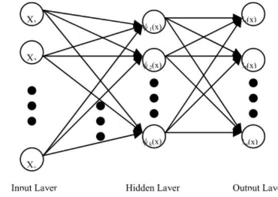
The radial basis function network (RBFN) is a special type of neural networks with several distinctive features [1], [2], [3], [4], [5], [6]. Since its first proposal, the RBFN has attracted a high degree of interest in research communities. An RBFN consists of three layers, namely the input layer, the hidden layer, and the output layer. The input layer broadcasts the coordinates of the input vector to each of the nodes in the hidden layer. Each node in the hidden layer then produces an activation based on the associated radial basis function. Finally, each node in the output layer computes a linear combination of the activations of the hidden nodes. How an RBFN reacts to a given input stimulus is completely determined by the activation functions associated with the hidden nodes and the weights associated with the links between the hidden layer and the output layer. The general mathematical form of the output nodes in an RBFN is as follows:
∑
=−
=
k i i i ji jx
x
c
1),
||;
(||
)
(
ω
φ
μ
σ
(1)
where cj(x) is the function corresponding to the j-th output unit (class-j)
and is a linear combination of k radial basis functions φ() with center μi and bandwidth σi. Also, wj is the weight vector of class-j and wji is the
weight corresponding to the j-th class and i-th center. The general architecture of RBFN is shown in Fig 1.
In this paper, we select the spherical (or symmetrical) Gaussian function as our basis function of RBFN, so the Eq.1 becomes:
∑
=−
−
=
k i i i ji jx
x
c
1 2 2)
2
||
||
exp(
)
(
σ
μ
ω
( 2 )From Eq.2, we can see that constructing an RBFN involves determining the number of centers, k, the center locations, μi, the
bandwidth of each center, σi, and the weights, wji. That is, training an
RBFN involves determining the values of three sets of parameters: the centers (μi), the bandwidths (σi), and the weights (wji), in order to
minimize a suitable cost function.
Basically, there are two categories of learning algorithms proposed for RBFNs [5], [7]. The first category of learning algorithms simply places one radial basis function at each sample [8], [9]. On the other hand, the second category of learning algorithms attempt to reduce the number of hidden nodes in the network, or equivalently the number of radial basis functions in the linear function above [10], [11], [12], [13], [14]. One primary motivation behind the design of the second category of algorithms is to reduce the complexity of the network constructed. The typical procedure incorporated in the second category of learning algorithms conducts a clustering analysis on the training instances and then allocates one hidden node for each cluster of instances. In this regard, the effects of a wide variety of clustering algorithms have been investigated [4], [15]. Nevertheless, both the conventional
agglomerative hierarchical clustering algorithm and the conventional partitional algorithm suffer some kinds of deficiencies. The main problem with the conventional agglomerative hierarchical clustering algorithm is its space complexity of O(n2), where n is the number of
training instances, due to the need to store pairwise distances or similarity scores between the training instances. The main problem with the conventional partitional clustering algorithm is that the user needs to figure
out how many clusters are appropriate for the given training data set. In 1997, Hwang et al. [12] proposed an incremental clustering based approach for determining the locations of hidden nodes in the RBFN to be constructed. The incremental approach enjoys several advantages. First, it does not need to compute all the pairwise distances or similarity scores between training instances. The key issue in this regard is that the space complexity for storing the pairwise distances or similarity scores is greatly reduced, in addition to lower time complexity. Second, it figures out the number of clusters automatically based on a user-specified parameter. Third, it executes more efficiently than the conventional agglomerative hierarchical clustering algorithm and the conventional partitional clustering algorithm. Nevertheless, the incremental clustering algorithm proposed by Hwang employs a fixed threshold of radius to control the formation of clusters. As a result, the clusters identified may not be well adapted to the local distributions of training instances. For example, in a region with a low local density of training instances, the threshold of radius for controlling the formation of clusters should be set to a large value. On the other hand, in a region with a high local density of training instances, the threshold of radius should be set to a small value.
This paper proposes a novel method to construct an RBFN classifier by using an incremental hierarchical clustering algorithm for constructing an RBFN optimized for data classification applications. Our contribution consists of two parts. The first one is an incremental hierarchical clustering algorithm that constructs the hidden layer effectively and efficiently. Since the clustering algorithm is hierarchical, the formation of clusters is controlled by the class labels of training samples instead of a fixed threshold and therefore the clusters identified are well adapted to the local distributions of training instances. In addition, because the clustering algorithm is incremental, it does not need to compute all the pairwise distances or similarity scores between training instances. The second part is
an improved least mean square error method that calculates the weights between the hidden and the output layers of an RBFN. In [12], authors proposed an improved method which uses a smaller matrix to compute the weights. The method proposed by [12] is more efficient and practical than the traditional one, but it may suffer the singular matrix problem and fails to build the classifier in such case. We solve the singular matrix problem by using the regularization theory in this paper, and then propose a method that can obtain the optimal weights analytically and efficiently.
Experimental results show that the data classifier constructed is capable of delivering comparable classification accuracy as the SVM [16] and the novel kernel density estimation (KDE) based classifier that we have recently proposed [8], while enjoying significant execution efficiency in handling data sets that contains a high percentage of redundant training instances. For example, in the experiment with the shuttle data set in the UCI repository [17], the mechanism proposed in this paper enjoys 1231 times and 259 times speedup over the SVM and the KDE based classifier that we have recently proposed, respectively, for constructing a data classifier. In addition, the mechanism proposed in this paper delivers comparable execution efficiency as the SVM in the prediction phase and enjoys 481 times speedup over the KDE based classifier in this regard. Experimental results also reveal that the approaches that have been proposed in recent years for solving the efficiency issues of the SVM and the KDE based classifier all lead to slight degradation of classification accuracy.
This paper is organized as follows. In next section, we introduce an incremental clustering method. In Section III and IV, we detail how to calculate the bandwidths and weights of
the radial basis functions which are employed in constructing the RBFN. Next, numerical experiments are shown in Section V. Finally, we have some discussions and conclusions in Section VI.
II. DETERMINING THE CENTERS
In the proposed hierarchical approach, a hierarchical agglomerative clustering (HAC) algorithm [18], [19] is invoked to cluster all the instances in training data set. After hierarchical clustering terminates, the class labels are applied to the dendrogram to derive target clusters. Each node in the clustering dendrogram corresponds to a cluster of data instances. A node in the dendrogram is identified as a target cluster if it contains only data instances from a single class and its parent does not satisfy the criterion. The centroids of the target clusters are used as the centers in constructing the hidden layer of RBFN. In this paper, the completelink algorithm [19] is employed. The reason of employing the complete-link algorithm is its tendency to find spherical clusters. Since the hierarchical clustering algorithms suffer higher time complexity, an incremental clustering framework for expediting the hierarchical clustering process is introduced as follows.
A. Incremental framework
We adopt the incremental framework proposed in our previous work [20]. This section describes how the incremental algorithm works. The incremental algorithm operates in two phases, initial phase and incremental phase. In both phases, it invokes the complete-link algorithm to construct a clustering dendrogram.
1) Initial phase: In the incremental algorithm, it is assumed that all the incoming data instances are first buffered in an incoming data pool. In the first phase of the algorithm, a number of data instances are taken from the incoming data pool and the complete-link algorithm is invoked to cluster these instances build a tentative dendrogram. We can assume that these data instances are selected sequentially according to the order of input sequence. As demonstrated in our previous work [20], the proposed incremental framework employs two operations, split and merge, to reduce the influence from input ordering. When the
criterion invoked in the first phase are invoked again to find the target clusters from the new tentative dendrogram. During the reconstruction process, two original target clusters will have chance to form a new bigger target cluster. This is regarded as the so-called merge operation.
The incremental phase repeats until there is no data instances left in the incoming data pool. After the clustering process terminates, the centroids of all the target clusters are collected as the centers of RBFN when constructing the classifier in the following sections.
III. CALCULATION OF THE BANDWIDTHS
For the hidden layer of the RBFN classifier, we use the proposed hierarchical approach to determine the number of the nodes and their center locations. Another parameter to be decided for each node in the hidden layer is the bandwidth of its kernel function, σi. Here, we employ the method presented by Moody and Darken [21] to determine the bandwidth of each kernel function. The bandwidth of a kernel
X1 X2 Xn ψ1(x) ψ2(x) ψk(x) C1(x) C2(x) Cm(x)
Input Layer Hidden Layer Output Layer
complete-link algorithm terminates, target clusters are derived by the method described above, i.e. the class labels are used to identify the cluster boundaries in the clustering hierarchy.
There are four pieces of information recorded for each target cluster: (1) the centroid, (2) the radius, (3) the class label and (4) the number of instances in the cluster. The radius of a cluster is defined to be the maximum distance between the centroid and the data instances in this cluster.
2) Incremental phase: In the second phase of the incremental algorithm, the data instances remained in the incoming data pool are examined one by one. For each new data instance, the algorithm will find its nearest neighbor in the set of target clusters. If the distance between the new data instance and its nearest target cluster is smaller than the radius of the target cluster, the new data instance is inserted into the target cluster. If not, the data instance is currently an outlier to the set of target clusters and is therefore put into the tentative outlier buffer temporarily. The data instance, however, may form a target cluster with other data instances that are already in the tentative outlier buffer or that come in later.
If a data instance is successfully inserted into an existing target cluster, we should check if the new data instance possesses the same class label with the other data instances in the target cluster. If not, an additional operation called split should be invoked to identify new target clusters in this local area. In the split operation, we apply the complete-link algorithm only to the data instances in this target cluster, and identify new target clusters with pure property as we did in the first phase. After the split operation finishes, the number of target clusters will increase at least by one.
Once the number of data instances in the tentative outlier buffer exceeds a threshold, the complete-link algorithm is invoked again to construct a new tentative dendrogram. In this reconstruction process, the primitive objects are the target clusters and the data instances in the tentative outlier buffer. In this case, each target cluster is represented by its centroid and regarded as a single data instance. When a new tentative dendrogram has been generated, the same procedure and
function is set as βdenemy, where denemy is the distance to the center of the nearest cluster which belong to a different class and β is a constant. In this paper, we follow the heuristic setting suggested by [12], i.e. β = 5.
IV. CALCULATION OF THE WEIGHTS
After the centers and bandwidths of the kernel functions in hidden layer have been determined, the transformation between the inputs and the corresponding outputs of the hidden units is now fixed. The network can thus be viewed as an equivalent single-layer network with linear output units. Then, we use the least mean square error method to determine the weights associated with the links between the hidden layer and the output layer.
In this section, we will show how the least mean square error method have been used in data classification field, and then propose a method which has a better theoretical foundation and practical use.
Assume h is the output of the hidden layer.
,
)]
(
...
)
(
2
)
(
[
1 T kx
x
x
h
=
φ
φ
φ
( 3 )where k is the number of centers, φ1(x) is the output value of first
kernel function with input x. Then, the discriminant function cj(x) of
class-j can be expressed by the following:
,
)
(
x
h
c
j=
ω
Tj j = 1 , 2 , . . . , m ( 4 )where m is the number of class, and wj is the weight vector
of class-j. We can show wj as:
T jk j j j
[
ω
1ω
2...
ω
]
ω
=
. ( 5 )After calculating the discriminant function value of each class, we choose the class with the biggest discriminant function value as the classification result. We will discuss how to get the weight vectors by using least mean square error method in the following subsections.
A. Traditional Least Mean Square Error Method
The traditional least mean square error method was proposed by Broomhead and Lowe [22]. This method is originally proposed for function approximation, and is the most popular supervised learning method of constructing the weights of RBFN [2], [3], [5], [23]. In this method, the objective function of class-j can be shown as:
2 1
]
)
(
)
(
[
min
∑
=−
n i i j i jx
v
x
c
(6) where⎪⎩
⎪
⎨
⎧
∈
−
=
1
0
.
,)
(
if
x
class
j
otherwise
x
v
j i . (7)This system is overconstrained, being composed of n equations with k unknown weights, then the optimal solution of wj can be written as
j
y
j
=
Φ
+
∗
ω
, (8) where yj = [ vj(x1) vj(x2) . . . vj(xn) ]T , Φli = φi(xl) and Φ+ is thepseudoinverse of Φ. The matrix Φ is rectangular (n×k) and its pseudoinverse can be computed as
Φ+ = (ΦT Φ)−1ΦT ,
provided that (ΦT Φ)−1 exists. The matrix (ΦT Φ) is square and its
dimensionality is k, so that it can be inverted in time proportional to k3.
Although in theory the quantity of (ΦT Φ)−1 exists, the cost of
computing Φ+ is very high. First, we need to store Φ of size (n×k) in the
To find the optimal W that minimizes J, we set the gradient of J(W ) to be zero:
∑
∑
= ==
−
=
∇
m j T j j j m j T j j wJ
W
P
E
hh
W
P
E
h
V
1 1]
0
[
}
{
2
}
{
2
)
(
, (11)where [0] is a k × m null matrix.
Let Ki denote the class-conditional matrix of the secondorder moments of h, i.e.
Ki = Ei {hhT }. (12)
If K denotes the matrix of the second-order moments under the mixture distribution, we have
∑
==
m j j jK
P
K
1 . (13) Then Eq. 11 becomesKW = M, (14) where
∑
==
m j T j j jE
h
V
P
K
1}
{
. (15) If K is nonsingular, the optimal W can be calculated byW∗ = K−1M. (16)
When compared to the traditional method, the size of K, k × k, is much smaller than the Φ matrix of size (n × k) described in the previous subsection. Therefore, the improved method requires less memory space for storing the matrix, as well as consumes much less
memory. The value of n in some classification problems is very large, such that it may be impractical to have such large amounts of memory space for storage. Also, the process of calculating (ΦT Φ)−1 for large Φ is
computationally expensive. In addition, this method needs a lot of computations for matrix multiplication and inversion. Therefore, this method may not be suitable for the use of classification problem.
B. Improved Least Mean Square Error Method
The improved least mean square error method for data classification was proposed by Devijver et. al.[24] and has been employed by Hwang et. al. in [12]. This method aims to calculate wj for m classes at the same
time. We detail the procedures as follows.
For a classification problem with m classes, let Vi designate the i-th
column vector of an m × m identity matrix and W be an k × m matrix of weights:
]
...
[
ω
1ω
2ω
mω
=
Then the objective function to be minimized is
∑
=−
=
m j j T j jE
W
h
V
P
W
J
1 2}
||
{||
)
(
, (10)where Pj and Ej{} are the a priori probability and the expected value of
class-j, respectively.
computation time for matrix multiplication. It is apparent that the improved method is more efficient than the traditional one.
However, there is a critical drawback of the improved method. That is, K may be singular and this will crash the whole procedure. By observing the matrix hhT, we are aware of that the matrix hhT is
symmetric positive semi-definite (PSD) matrix with rank = 1. Since K is the summation of hhT for each training instance, K is also a PSD
matrix with rank ≤ n. When k → n, it is highly possible to have K be singular. From our experiences, if all the training instances are chosen as centers, this method is not going to work eventually. Thus, we solved this problem in the following subsection.
C. Proposed Least Mean Square Method
A very simple solution to solve the singular problem has been shown in the context of regularization theory [25]. It consists in replacing the the objective function as follows:
∑
∑
= =+
−
=
m j j T j m j j T j jE
W
h
V
P
W
J
1 1 2}
||
{||
)
(
λ
ω
ω
, (17)where λ is the regularization parameter. Then the Eq. 14 becomes (K + λI)W = M. (18)
TABLE I
THE BENCHMARK DATA SETS USED IN THE EXPERIMENTS If we set λ > 0, (K + λI) will be a positive definite (PD) matrix and therefore is nonsingul ar. The optimal W ∗ can be calculated by W∗ = (K + λI)−1M. (19)
Finally, we can get the optimal
W
j*for class-j from W∗, and thenthe optimal discriminant function cj(x) for class-j is derived. By using
the regularization theory, the optimal weights can be obtained analytically and efficiently.
V. EXPERIMENTS IN THE PROBLEM OF DATA CLASSIFICATION
The experiments in this section are conducted to evaluate the performance of the proposed RBFN classifier against other famous classifiers, the KDE based classifier [8], SVM [16], and KNN. Also, the incremental hierarchical clustering algorithm is compared with the APC-III clustering algorithm employed in [12]. Our proposed RBFN classifier and the APCIII based classifier share the same procedures of determining bandwidths and weights in constructing the RBFN. The discussions of the experiments will focus on the following two issues: classification accuracy and execution efficiency.
Table I lists main characteristics of the nine benchmark data sets used in the experiments. All these data sets are from the
UCI repository [17]. Among the nine data sets, three of them are considered as the larger ones, as each contains more than 5000 samples with separate training and testing subsets. The remaining six data sets are considered as the smaller ones and there are no separate training and testing subsets in these six smaller data sets. Accordingly, different evaluation practices have been employed for the smaller data sets and for the larger
data sets. For the three larger data sets, 10-fold cross validation has been conducted on the training set to determine the optimal parameter values
# of training samples # of testing samples satimage 4435 2000 letter 15000 5000 shuttle 43500 14500 iris 150 N/A wine 178 N/A vowel 528 N/A segment 2310 N/A glass 214 N/A vehicle 846 N/A TABLE II
COMPARISON OF CLASSIFICATION ACCURACY WITH THE THREE LARGER
DATA SETS TABLE III
COMPARISON OF CLASSIFICATION ACCURACY WITH THE SIX SMALLER
DATA SETS
KDE SVM 1NN 3NN APC-III Proposed
iris 97.33 97.33 96.00 95.33 95.33 96.00 wine 99.44 99.44 95.52 96.07 98.89 97.78 vowel 99.62 99.05 99.62 97.35 93.37 98.48 segment 97.27 97.40 97.27 96.14 94.98 97.53 glass 75.74 71.50 72.01 92.01 69.16 72.86 vehicle 73.53 86.64 69.73 71.39 78.25 79.19 Average 90.49 91.89 88.36 88.05 88.33 90.31
the size of training data set is larger than 20000. In regard to the parameter settings of other classifiers for comparison, we adopted the parameter settings suggested by the authors in their original papers.
Table II compares the accuracy delivered by alternative classification algorithms with the three larger benchmark data sets. As Table II shows, the proposed method basically deliver the same level of accuracy with other famous classifiers, SVM and KDE, while the KNN and APC-III based classifier do not produce comparable generation results. Table III lists the experimental results with the six smaller data sets. Table III shows that the proposed method basically deliver the same level of accuracy for these six data sets. The experimental results presented in Table III also show that the proposed method, KDE based classifier and the SVM generally deliver a higher level of accuracy than the KNN and APC-III based classifier.
Table IV compares the execution time of the KDE based classifier, the SVM, the APC-III based classifier and the proposed method with the three larger data sets presented in Table I. In Table IV, the total
KDE SVM 1NN 3NN APC-III Proposedd
satimage 92.30 91.30 88.80 90.65 90.25 92.00 letter 97.12 97.98 95.68 95.16 91.16 97.48 shuttle 99.94 99.92 99.94 99.91 97.34 99.82 Average 96.45 96.40 94.84 95.24 92.92 96.43
to be used in the testing phase. On the other hand, for the six smaller data sets, 10-fold cross validation has been conducted on the entire data set and the average result is reported.
Our incremental algorithm has two key parameters, the size of initial data samples and the size of the tentative outlier buffer. In our experiments, both of the size of initial data instances and the size of tentative outlier buffer are set to 1000. We observed that these two buffers do not affect the quality of the classifier much but do influence the execution time. The larger the buffer size, the longer the reconstructing process. In the experiments, the incremental mechanism is turned on when
time taken to construct classifiers based on the given training data sets are listed in the rows marked by "Make classifier". The time listed in "Make classifier" row are the time of cross validation for KDE based classifier and the time of model selection for SVM. On the other hand, for both the APC-III based classifier and the proposed algorithm, the reported time include the time of clustering process and the time of calculting bandwidths and weights. In addition, the time taken by alternative classifiers to predict the classes of the testing instances are listed in the rows marked by "Prediction".
As we can see in Table IV, the mechanism proposed in this paper is much more efficient than the SVM and the KDE based classifier for constructing a data classifier. In addition, the mechanism proposed in this paper delivers comparable execution efficiency as the SVM in the prediction phase and
TABLE IV
COMPARISON OF EXECUTION TIME IN SECONDS
KDE SVM APC-III Proposed
satimage 676 64644 136 274 letter 2842 387096 712 5244 Make Classifier shuttle 98540 467955 2595 380 satimage 21.30 11.53 0.63 7.06 letter 128.60 94.91 2.15 28.06 Prediction Time shuttle 996.10 2.13 0.48 2.07
enjoys 30 times speedup over the KDE based classifier in this regard.
VI. CONCLUSION
In this paper we present an efficient method to construct an RBFN classifier whose performance was shown to be as good as the existing classification methods on the data sets used in this paper. Our contribution consists of two parts. First, we propose an incremental hierarchical clustering algorithm for constructing the hidden layer effectively and efficiently. Second, an improved least mean square error method that calculates the weights between the hidden and the output layers of an RBFN is introduced.
In the proposed clustering approach, the formation of clusters is controlled by the class lables of training samples and therefore the clusters identified are well adapted to the local distributions of training instances. In addition, it does not need to compute all the pairwise distances or similarity scores between training instances. Experimental results show that the data classifier constructed is capable of delivering comparable classification accuracy as the SVM and the kernel density estimation based classifier that we have recently proposed, while enjoying significant execution efficiency in handling data sets that contains a high percentage of redundant training instances.
Also, the proposed least mean square error method is efficient and with good theoretical foundations. The traditional least mean square method requires large memory to store the matrix and consumes a lot of execution time for the matrix multiplications and inversions. The improved method proposed by [12] is more efficient and practical than the traditional one, but it may suffer the singular matrix problem and fails to build the classifier in such case. In this paper, we solve the singular matrix problem by using the regularization theory, and this provides a good framework for constructing an RBFN in classification problems.
Experimental results also reveal that the approaches that have been proposed in recent years for solving the efficiency issues of the SVM and the kernel density estimation based mechanism all lead to slight degradation of classification accuracy. Thus, how to improve the efficiency of learning algorithms without sacrificing classification accuracy still deserves further studies.
REFERENCES
[1] J. Park and I. W. Sandberg, “Universal approximation using radial-basisfunction networks,” Neural Computation, vol. 3, no. 2, pp. 246–257, 1991.
[2] T. Poggio and F. Girosi, “A theory of networks for approximation and learning,” Tech. Rep. A.I. Memo 1140, Massachusetts Institute of Technology, Artificial Intelligence Laboratory and Center for Biological Information Processing, Whitaker College, Jul 1989.
[3] J. Ghosh and A. Nag, “An overview of radial basis function networks,” Radial Basis Function Neural Network Theory and Applications, R. J. Howlerr and L. C. Jain (Eds), 2000. [4] T. M. Mitchell, Machine Learning. McGraw-Hill, 1997.
[5] M. J. L. Orr, “Introduction to radial basis function networks,” tech. rep., Center for Cognitive Science, University of Edinburgh, UK, 1996.
[6] V. Kecman, Learning and Soft Computing: Support Vector Machines, Neural Networks, and Fuzzy Logic Models. The MIT Press, 2001.
[7] C. M. Bishop, “Improving the generalization properties of radial basis function neural networks,” Neural Computation, vol. 3, no. 4, pp. 579– 588, 1991.
[8] Y.-J. Oyang, S.-C. Hwang, Y.-Y. Ou, C.-Y. Chen, and Z.-W. Chen, “Data classification with radial basis function networks based on a novel kernel density estimation algorithm,” IEEE Transactions on Neural Networks, pp. 225 – 236, 2005.
[9] D. G. Lowe, “Similarity metric learning for a variable-kernel classifier,” Neural Computation, vol. 7, pp. 72–85, 1995.
[10] A. Lyhyaoui, M. Martinez, I. Mora, M. Vazquez, J.-L. Sancho, and A. R. Figueiras-Vidal, “Sample selection via clustering to construct support vector-like classifiers,” IEEE Transactions on Neural Networks, vol. 10, p. 1474, Nov 1999.
[11] S. Chen, C. F. N. Cowan, and P. M. Grant, “Orthogonal least squares learning algorithm for radial basis function networks,” IEEE Transactions on Neural Networks, vol. 2, pp. 302–309, Mar. 1991.
[12] Y. Hwang and S. Bang, “An efficient method to construct a radial basis function neural network classifier,” Neural Networks, vol. 10, no. 8, pp. 1495–1503, 1997.
[13] M. J. L. Orr, “Regularisation in the selection of radial basis function centres,” 1995. [14] E. I. Chang and R. P. Lippmann, “A boundary hunting radial basis function classifier which allocates centers constructively,” in Advances in Neural Information Processing Systems, vol. 5, pp. 131–138, Morgan Kaufmann, San Mateo, CA, 1993.
[15] I. H. Witten and E. Frank, Data mining. Los Altos, US: Morgan Kaufmann, 2000. [16] C.-W. Hsu and C.-J. Lin, “A comparison of methods for multi-class support vector machines,” IEEE Transactions on Neural Networks, vol. 13, no. 2, pp. 415–425, 2002. [17] C. L. Blake and C. J. Merz, “UCI repository of machine learning databases,” tech. rep., University of California, Department of Information and Computer Science, Irvine, CA, 1998. Available at http://www.ics.uci.edu/~mlearn/MLRepository.html.
[18] A. K. Jain, M. N. Murty, and P. J. Flynn, “Data clustering: a review,” ACM Computing Surveys, vol. 31, pp. 264–323, Sept. 1999.
[19] A. K. Jain and R. C. Dubes, Algorithms for Clustering Data. Prentice Hall International, 1988.
[20] C.-Y. Chen, S.-C. Hwang, and Y.-J. Oyang, “An incremental hierarchical data clustering algorithm based on gravity theory,” in Proc. of PAKDD- 2002, pp. 237–250, 2002. [21] J. Moody and C. J. Darken, “Fast learning in networks of locally-tuned processing units,” Neural Computation, vol. 1, no. 2, pp. 281–294, 1989.
[22] D. S. Broomhead and D. Lowe, “Multivariable functional interpolation and adaptive networks,” Complex Systems, vol. 2, pp. 321–355, 1988.
[23] I. Tarassenko and S. Roberts, “Supervised and unsupervised learning in radial basis function classifiers,” in IEE Proceedings-Vision, Image and Signal Processing, vol. 141, pp. 210–216, 1994.
[24] P. A. Devijver and J. Kittler, Pattern recognition : a statistical approach. Prentice Hall, 1982.
[25] A. N. Tikhonov and V. Y. Arsenin, Solutions of Ill-Posed Problems. Washington D.C.: V.H. Winston & Sons, John Wiley & Sons, 1977.