臺灣國際觀光旅館住用率研究

(1)

Taiwan International Hotel Occupancy Rate Reserch

D9860195 D982195没 D98219没4 D9860458 D98219没9

Statistical Methods For Forecasting

(2)

1999 1 2012 3 159 ARIMA

(3)

Abstract

The principal aim of this paper is to research the occupancy rate of international hotel in Taiwan. All the data and related information have been retrieved from the websites of the Tourism Bureau, Ministry of Transportation of Republic of China including the monthly statistics operation reports . We only gathered t the occupancy rate of international hotel in Taiwan between January 1999 to March 2012. These data contain 159 monthly data.

In this research four common types of forecast measurement were used the ARIMA Model Analysis Method, the Time Series Regression Method, the Exponential Smoothing Method and the Decomposition Method.

Autocorrelation of each model was taken and the their respective predictions compared to the real values. Furthermore, we used the

forecast evaluation instruction to determine the most appropriate forecast model.

As a result, the most appropriate model to predict the occupancy rate of international hotel in Taiwan is the Time Series Regression Method. It accurately predicted the future occupancy rate twelve times.

Keywords International hotel. Occupancy rate. Statistic forecast.

(4)

06 06 06 06 06060606 09090909 10101010 11111111 12121212 12121212 12121212 14141414 15151515 16161616

ARIMAARIMAARIMAARIMA 20202020 202020 20 2没2没2没2没

1111 White Noise TestWhite Noise TestWhite Noise TestWhite Noise Test 2没2没2没2没

2222 Unit Root TestUnit Root TestUnit Root TestUnit Root Test 28282828 3

33

3 LjungLjungLjungLjung----BoxBoxBoxBox 28282828 24242424 31313131

Time Series RegrTime Series RegrTime Series RegrTime Series Regressionessionessionession 32323232 32323232 34343434 36363636 38383838

Decomposition MethodDecomposition MethodDecomposition MethodDecomposition Method 39393939 39393939 45454545 46464646 4没4没4没4没

Exponential SmoothingExponential SmoothingExponential SmoothingExponential Smoothing 49494949 49494949 52525252 53535353 54545454 55555555 55555555 5没 5没 5没 5没 5没 5没5没 5没 58 5858 58

(5)

Figure 01 Figure 01Figure 01 Figure 01 11111111 Figure 02 Figure 02Figure 02 Figure 02 13131313 Figure 03 Figure 03Figure 03

Figure 03 ACF ACF ACF ACF PACFPACFPACFPACF 22222222 Figure 04

Figure 04Figure 04

Figure 04 ACFACFACFACF PACFPACFPACFPACF 23232323 Figure 0

Figure 0Figure 0

Figure 05555 ARIMAARIMAARIMAARIMA ACF&PACFACF&PACFACF&PACFACF&PACF 24242424 Figure 06

Figure 06Figure 06

Figure 06 ARIMAARIMAARIMAARIMA 26262626

Figure 0没 Figure 0没Figure 0没

Figure 0没 ARIMAARIMAARIMAARIMA White NoiseWhite NoiseWhite NoiseWhite Noise Unit RootUnit RootUnit RootUnit Root 29292929 Figure 08

Figure 08Figure 08

Figure 08 ARIMAARIMAARIMAARIMA 1111 32323232 Figure 09 Figure 09Figure 09 Figure 09 2222 38383838 Figure 10 Figure 10Figure 10 Figure 10 40404040 Figure 11 Figure 11Figure 11 Figure 11 41414141 Figure 12 Figure 12Figure 12 Figure 12 42424242 Figure 13 Figure 13Figure 13 Figure 13 43434343 Figure 14 Figure 14Figure 14 Figure 14 43434343 Figure 15 Figure 15Figure 15 Figure 15 3333 48484848 Figure 16 Figure 16Figure 16 Figure 16 51515151 Figure 1没 Figure 1没Figure 1没

Figure 1没 ACFACFACFACF PACFPACFPACFPACF 52525252 Figure 18

Figure 18Figure 18

(6)

Table 01 Table 01Table 01 Table 01 3333 09090909 Table 02 Table 02Table 02 Table 02 12121212 Table 03 Table 03Table 03

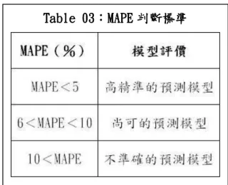
Table 03 MAPEMAPEMAPEMAPE 18181818

Table 04 Table 04Table 04

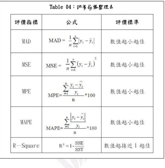
Table 04 19191919

Table 05 ARIMAARIMAARIMAARIMA 1111 30303030

Table 06 ARIMAARIMAARIMAARIMA 1111 31313131 Table 0没 Table 0没Table 0没 Table 0没 36363636 Table 08 Table 08Table 08 Table 08 2222 1111 3没3没3没3没 Table 09 Table 09Table 09 Table 09 2222 222 2 3没3没3没3没 Table 10 Table 10Table 10 Table 10 2222 38383838 Table 11 Table 11Table 11 Table 11 46464646 Table 12 Table 12Table 12 Table 12 3333 1 1 1 1 4没4没4没4没 Table 13 Table 13Table 13 Table 13 3333 2 2 2 2 4没4没4没4没 Table 14 Table 14Table 14 Table 14 3333 48484848 Table 15 Table 15Table 15 Table 15 4444 53535353 Table 16 Table 16Table 16 Table 16 4444 54545454 Table 1没 Table 1没Table 1没 Table 1没 55555555

(7)

Room Occupancy Rate

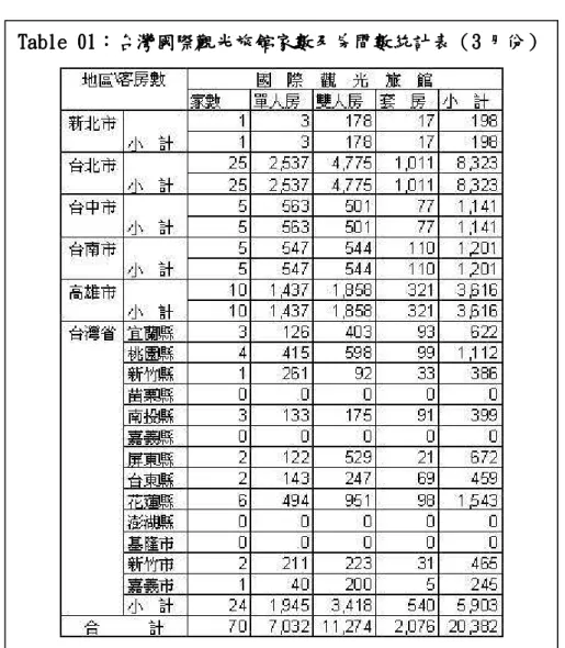
= / × 100 300 6 5,310 6 59

(8)

(9)

2016 608 1,000 3,000 没0 25 8,323 4 没38 2.91% 10 3,616 2 394 2.0没% Table 01

4,000

(10)

Table 01 Table 01 Table 01 Table 01 3333

(11)

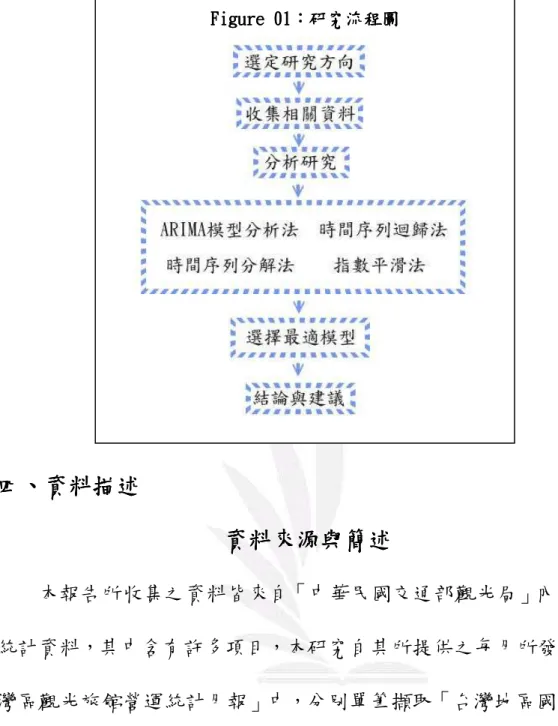
Figure 01 1 2 3 ARIMA 4 5

(12)

Figure 01 Figure 01 Figure 01 Figure 01

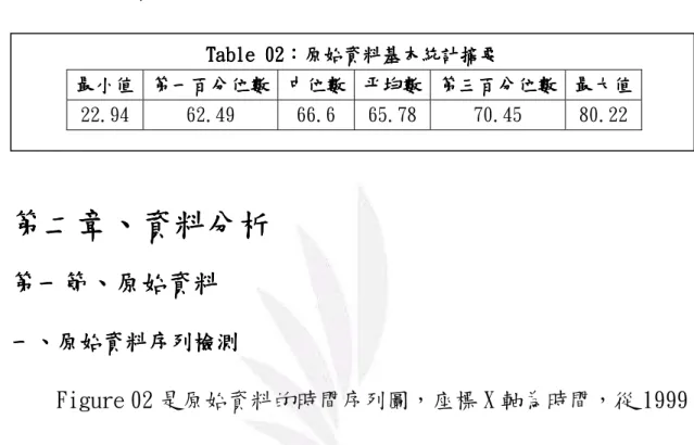
1999 1 2012 3 159 2011 4 2012 3 12 Table 02 Figure 01 2011

(13)

Table 02 Table 02Table 02 Table 02 22.94 62.49 66.6 65.没8 没0.45 80.22 没5.45% 没1.46% 66.53% 68.55% 36.没1% 62.3没% 61.21% 59.3没%

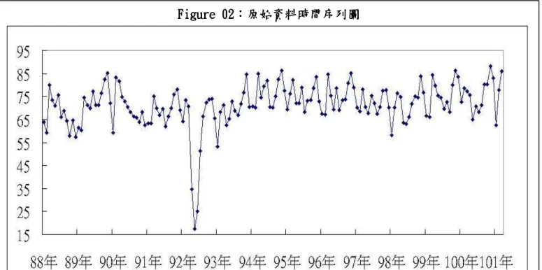
Figure 02 X 1999 1 2012 3 Y Figure 01 2003 4 5 6 SARS

(14)

Log 1~3 6~9

(15)

Figure 01 2003 4 5 6 ARIMA SAS

(16)

Trading-day 31 29

(17)

12 12

12

1.MAD Mean Absolute Deviation

2.MSE Mean Squared Errorr 3. MPE Mean

Percentage Error 4. MAPE Mean Absolute Percentage

Error 5.R-Square Coefficient of Determination

1

n

t

y i yˆ_t i

(18)

2 MSE Mean Squared Errorr

3 MPE Mean Percentage Error

4 MAPE Mean Absolute Percentage Error

(19)

Table 03 MAPEMAPEMAPEMAPE

5 R Square Coefficient of Determination 2 R (Goodness of Fit) 0 R2 = (Y) (X) 0 R2 ≠ (Y) (X) SSE SST 2 R Table 04

(20)

Table 04 Table 04 Table 04 Table 04

(21)

ARIMA

ARIMA ARIMAARIMA ARIMA

ARIMA Autoregressive Integrated

Moving Average Model ARIMA Box-Jenkins

ARIMA ARIMA 1 AR Model 2 MA Model 3 ARIMA Model ARIMA ARIMA 1 ARIMA 2 3

(22)

4 ARIMA p d q AR , p ; MA q d ACF ACF ACF

ACF PACFPACFPACFPACF

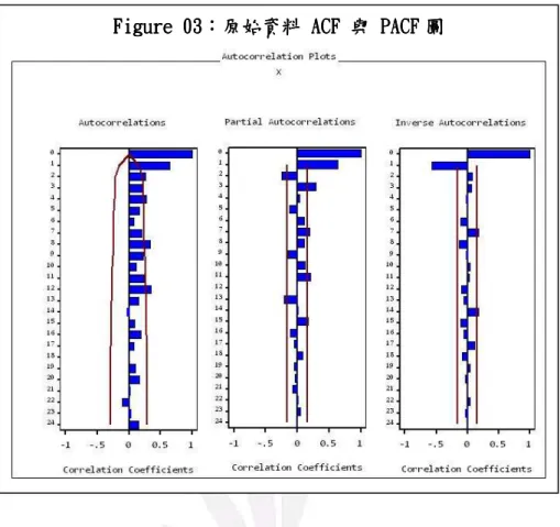
Figure 03 ACF PACF

ACF Lag12 1

(23)

Figure 0 Figure 0 Figure 0

Figure 03333 ACF ACF ACF ACF PACFPACFPACFPACF

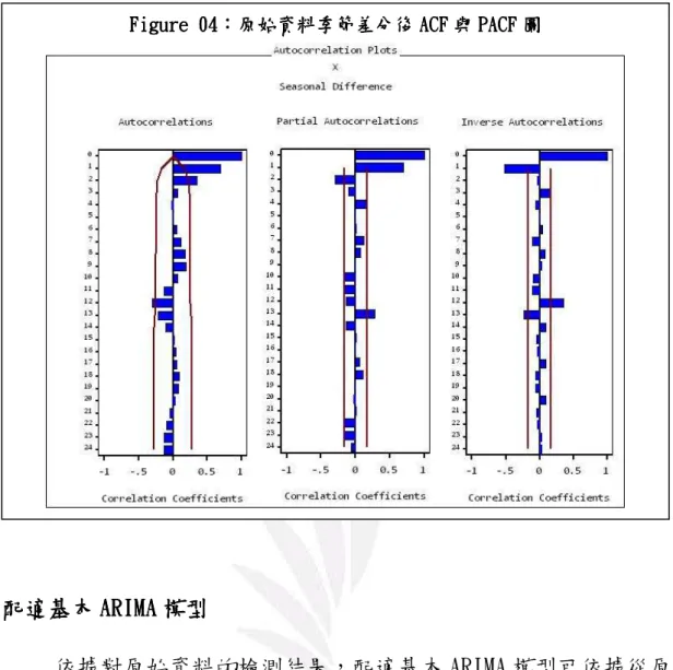
Figure 04 ACF PACF

ACF Lag2

(24)

Figure 04 Figure 04Figure 04

Figure 04 ACFACFACFACF PACFPACFPACFPACF

ARIMA ARIMA ARIMA ARIMA

ARIMA 1 ACF PACF ARIMA ARIMA ARIMA

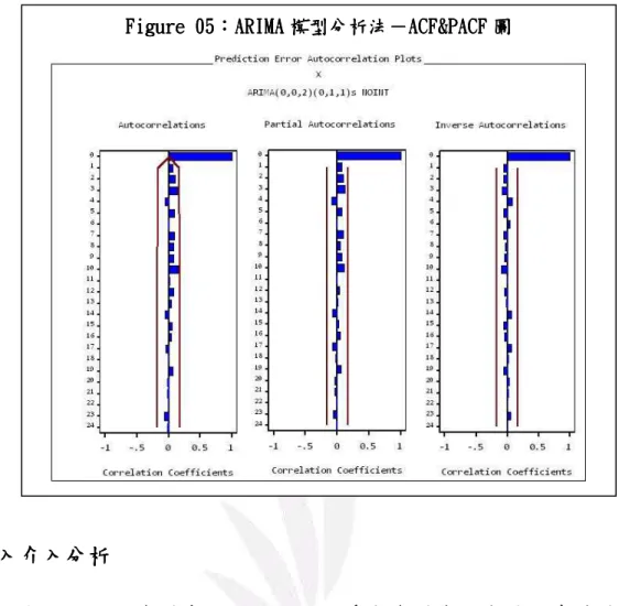
ARIMA 0,0,20,0,20,0,20,0,2 0000,1,,1,,1,1,1,111 s NOINTs NOINTs NOINTs NOINT

Figure 05 ARIMA

(25)

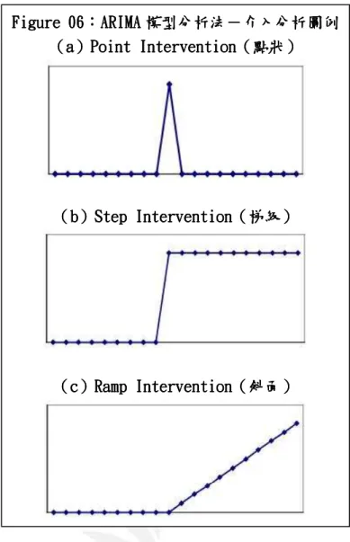
ARIMA 1 Point Intervention 1 Figure 06 a Figure 05 Figure 05 Figure 05

Figure 05 ARIMAARIMAARIMAARIMA ACF&PACFACF&PACFACF&PACFACF&PACF

(26)

   = = Otherwise , 0 t t if , 1 X_i.t int 2 Step Intervention 1 Figure 06 b    ≥ = Otherwise , 0 t t if , 1 X_i.t int 3 Ramp Intervention Figure 06 c    ≥ = Otherwise , 0 t t if , t -t

X_i.t int int

(27)

Point Intervention ARIMA ARIMA ARIMA Figure 06 Figure 06 Figure 06

Figure 06 ARIMAARIMAARIMAARIMA a

aa

a Point InterventionPoint InterventionPoint InterventionPoint Intervention

b bb

b Step InterventionStep InterventionStep InterventionStep Intervention

c cc

c Ramp InterventionRamp InterventionRamp InterventionRamp Intervention

(28)

White Noise Unit Root

1111 White NoiseWhite Noise White NoiseWhite Noise TestTestTestTest White Noise Noise. not White is a : H Noise. White is a : H t a t 0 P-Value 0.05 P-Value 0.05

Figure 0没 Lag P-Value

α=0.05 White Noise

(29)

2222 Unit RootUnit RootUnit RootUnit Root TesTesTesTestttt Unit Root ARIMA

(

)

(

Stationary

)

Root. Unit No : H Stationary Non Root. Unit : H a 0 P-Value 0.05 P-Value 0.05

Figure 0没 Lag P-Value

α=0.05

3 33

3 LjungLjungLjungLjung----BoxBoxBoxBox

(30)

Figure 0没 Figure 0没 Figure 0没

Figure 0没 ARIMAARIMAARIMAARIMA White NoiseWhite NoiseWhite NoiseWhite Noise Unit RootUnit RootUnit RootUnit Root

: H₀ : H_a P-Value 0.05 P-Value 0.05 α=0.05 Lag P-Value 0.05 ARIMA

(31)

Table 05 ARIMA ARIMA P-Value α=0.05 ARIMA Table 05 ARIMA ) B -(1 ) 0.82403B -)(1 0.44685B 0.82153B (1 P 0.81390B -1 15.37809 -P 0.81390B -1 15.37809 -P 0.81390B -1 15.37809 -yˆ 12 12 2 (54) t (53) t (52) t t + + + + + = 1 11 1    ₌ = Otherwise 0 52,53,54 i if 1 Pt(i)

19.40801

ˆ

=

σ

Table 05 Table 05 Table 05

Table 05 ARIMAARIMAARIMAARIMA 1111

(32)

Table 06 Table 06 Table 06

Table 06 ARIMAARIMAARIMAARIMA 1111

ARIMA 12 95 Table 06 ARIMA 12 95 Figure 08 ARIMA Figure 08 ARIMA 95

(33)

Figure 0 Figure 0 Figure 0

Figure 08888 ARIMAARIMAARIMAARIMA 1111

2011 9 95

Time Series Regression

(34)

Trend TRt Season SNt εt t t t t TR SN y = + +ε y_t t TR_t t SN_t t ε_t t t 11 12 1 2 1 0 t t d ... d yˆ =β +β +β + +β +ε       = =    =    = Otherwise 0, Nov when 1, d , ... , Otherwise 0, Mar when 1, d , Otherwise 0, Feb when 1, d , Otherwise 0, Jan when 1, d1 2 3 11 DW Pr DW α =0.05

(35)

2003 4 5 6 2003 4 52 2003 6 54    ≤ ≤ = Otherwise 0 54 t 52 if 1 I_t

(36)

Durbin DurbinDurbin

Durbin----WatsonWatsonWatson DWWatson DWDWDW DW

PR DW α =0.05

(37)

Table 0没 Table 0没 Table 0没 Table 0没 2 Table 0没 DW 1.9956 P-Value 0.05

Table 08 1 P-Value α =0.05 Table 08 Table 09 t t 11 10 9 8 7 6 5 4 3 2 1 t 15.0278I 5.1178d 1.5016d 2.5110d -0.1961d 1.3119d 0.1517d 3.7473d -1.7242d -1.8917d 2.0079d -8.0184d -0.0451t 63.0520 yˆ ε + + + + + + + =

(38)

Table 08 Table 08 Table 08 Table 08 2222 1111 a 0.041057 -0.649019 _t_-₁ _t_-₂ _t t = ε ε + ε at

~~

~

( )

2 0, N σ

0.05344 ˆ = σ

   ≤ ≤ = Otherwise 0 54 t 52 if 1 I_t

P-Value α=0.05 t d1 d11 It t I

Table 09 Table 09 Table 09 Table 09 2222 222 2

(39)

逢甲大學學生報告 ePaper(2012 年) 38 -Table 10 Table 10Table 10 Table 10 2222

12 Table 10 12 95 Figure 09 Figure 09 Figure 09Figure 09 Figure 09 2222

(40)

Figure 09 95

Decomposition Method

t y

(

t t t t

)

t f TR ,SN ,CL ,IR y = TRt Trend SNt Season CLt Cyclical IRt Irregular X11

(41)

Additive Model yt =TRt +SNt +CLt +IRt Multiplicative Model yt =TRt×SNt×CLt ×IRt

Figure 10 Figure 10 Figure 10 Figure 10 Figure 10

(42)

Figure 11

(43)

Figure 12 2005

(44)

Figure 13

(45)

Figure 14 2003 SARS 2003 4 5 6 2003 4 52 2003 6 54

(46)

   ≤ ≤ = Otherwise 0 54 t 52 if 1 I_t

DW P-Value PR DW α =0.05 PR DW α =0.05 Table 11

(47)

Table 11 Table 11Table 11 Table 11 DW 2.0139 P-Value 0.05

Table 12 1 P-Value α =0.05 Table 12 Table 13 1 t t 62.2206 0.0469t-15.7058I dy = + +ε

3333

t 2 -t 1 -t t =0.640368ε -0.017414ε +a ε

at

~~

~

( )

2 0, N σ

   ≤ ≤ = Otherwise 0 54 t 52 if 1 I × =

(48)

4.04846 2 = σ

12 12 Table 14 95 Figure 15

Table Table Table Table 11112222 3333 1111 Table 1 Table 1 Table 1 Table 13333 3333 2222

(49)

Figure 15 95

Figure 15 Figure 15Figure 15 Figure 15 3333

(50)

Exponential Smoothing

1 Winters Method Additive

2 Winters Method Multiplicative

(51)

1 and 0 between constant Smoothing & alue Forecast v F t period in series time the of factor seasonal The S rate growth The b level The L m t t t t = = = = = + γ α Figure 16 Figure 12

Winters Method Additive

Winters Method Multiplicative

(52)

Winters Method Additive

Zero-one/Additive 0.001

0.999 Additive Invertible Region

(53)

Figure 1没 Figure 1没Figure 1没

Figure 1没 ACFACFACFACF PACFPACFPACFPACF R-Square

Winters Method Multiplicative

Unrestricted

Winters

Method Additive

Figure 1没 ACF PACF Lag

Lag3

(54)

Table 15 P-Value α =0.05 25.38984 ˆ 80.19672 ˆ -0.00764 ˆ 0.99950 ˆ = γ = δ = σ2 = α

m s -t t t m t s -t 1 -t t t 1 -t 1 -t t t 1 -t 1 -t s -t t t m)S b (L F : Forecast S 79.19672 -) L / 80.19672(Y S : Seasonal b 1.00764 ) L --0.00764(L b : Trend ) b 0.0005(L ) S / 0.99950(Y L : Level + + = + = + = + + =

= αˆ γˆ= δˆ=

4 44 4

(55)

Table Table Table Table 16161616 4444 Figure 18 Figure 18Figure 18 Figure 18 4444

12 12 Table 16 12 95 Figure 18

(56)

Table 1没 Table 1没 Table 1没 Table 1没

Figure 18 95

MAD MSE MPE MAPE R-Square

Table 16

(57)

1没 MAD MSE MPE MAPE