ㄧ個只花O(log N)時間找出具有N點之雙環式網路的steps的演算法以及Hyper-L1三環式網路的存在性的探討

全文

(1)國立交通大學應用數學系碩士論文ㄧ個只花 O(log N)時間找出具有 N 點之雙環式網路的 steps 的演算法以及 Hyper-L1 三環式網路的存在性的探討 An O(log N)-Time Algorithm to Find the Steps of a Double-Loop Network with N Nodes and the Existence of Hyper-L1 Triple-Loop Networks. 研究生：唐文祥指導老師：陳秋媛. 教授. 中華民國九十三年六月.

(2) ㄧ個只花 O(log N)時間找出具有 N 點之雙環式網路的 steps 的演算法以及 Hyper-L1 三環式網路的存在性的探討 An O(log N)-Time Algorithm to Find the Steps of a Double-Loop Network with N Nodes and the Existence of Hyper-L1 Triple-Loop Networks 研究生：唐文祥. Student: Wen-Shiang Tang. 指導老師：陳秋媛教授. Advisor: Dr. Chiuyuan Chen. 國立交通大學應用數學系碩. 士. 論. 文. A Thesis Submitted to Department of Applied Mathematics College of Science National Chiao Tung University In partial Fulfillment of Requirement For the Degree of Master In Applied Mathematics June 2004 Hsinchu, Taiwan, Republic of China. 中華民國九十三年六月.

(3) ㄧ個只花 O(log N)時間找出具有 N 點之雙環式網路的 steps 的演算法以及 Hyper-L1 三環式網路的存在性的探討研究生：唐文祥. 指導老師：陳秋媛. 教授. 國立交通大學應用數學系摘. 要. 雙環式網路及三環式網路是許多學者專家廣泛探討的區域網路架構。給定一個正整數 N，找出具有 N 點、直徑最小的雙環式網路 DL(N;s1,s2)的 s1 和 s2（又稱為 steps）是學者專家們ㄧ直以來所想達成的目標。已知雙環式網路的 minimum distance diagram 是 L-型；對於雙環式網路而言，直徑可以很容易的由它的 L-型計算出。因此「找出具有 N 點、直徑最小的雙環式網路」的一個常見的方法是：將此問題轉換為「先找出一個直徑相當不錯的 L-型，再找出與這個 L-型對應的雙環式網路 DL(N; s1, s2)的 s1 和 s2 」。給定一個雙環式網路 DL(N; s1, s2)，在論文[8]中，Cheng 和黃光明老師提出了一個漂亮而且只花 O(log N)時間、找出對應的 L-型的演算法。但是，「給定一個 L-型，是否能夠只花 O(log N)時間，找出與這個 L-型相對應的雙環式網路 DL(N; s1, s2)的 steps」，卻一直是一個 open problem [5]。在這篇論文裡，我們提出一個只花 O(log N) 時間、找出與一個給定的 L-型相對應的雙環式網路 DL(N; s1, s2)的 steps 的演算法。令 N(D)表示一個直徑為 D 的三環式網路所能包含的最多點數。Hyper-L 型已被多位學者發現為推導出 N(D)的下界的一個有效的工具。然而，並非每一個 Hyper-L 型都會有一個三環式網路來得到它。截至目前為止，共有三種 hyper-L 型被學者們提出來，為了方便起見，我們分別稱它們為 hyper-L0、hyper-L1、hyper-L2。在論文[7]中，陳秋媛老師、黃光明老師、李珠矽老師、以及石舜仁學長提出了 hyper-L0 三環式網路存在的充份必要條件。在這篇論文裡，我們提出 hyper-L1 三環式網路存在的充份必要條件。. 關鍵詞：雙環式網路、L-型、直徑、演算法、三環式網路、hyper-L 型. 中華民國九十三年六月 i.

(4) An O(log N)-Time Algorithm to Find the Steps of a Double-Loop Network with N Nodes and the Existence of Hyper-L1 Triple-Loop Networks Student : Wen-Shiang Tang. Advisor : Dr. Chiuyuan Chen. Department of Applied Mathematics National Chiao Tung University Hsinchu 300, Taiwan, R.O.C.. Abstract Double-loop networks and triple-loop networks have been widely studied as architecture for local area networks. Given an N, it is desirable to find a double-loop network DL(N; s1, s2) with its diameter being the minimum among all double-loop networks with N nodes. It is well known that the minimum distance diagram of a double-loop network yields an L-shape. Since the diameter can be easily computed from an L-shape, one method is to start with a desirable L-shape and then asks whether there exist s1 and s2 (also called the steps of the double-loop network) to realize it. While Cheng and Hwang [8] have given an elegant O(log N)-time algorithm to find the L-shape of a double-loop network DL(N; s1, s2), it is an open problem whether the steps of a double-loop network with N nodes can be found in O(log N) time [5]. In this thesis, we propose an O(log N)-time algorithm to find the steps of a double-loop network with N nodes. Hyper-L tiles were proven to be an effective tool to obtain lower bounds for N(D), the maximum number of nodes in a triple-loop network with diameter D. Unfortunately, not every hyper-L tile has a triple-loop network realizing it. Up to now, three types of hyper-L tiles have been proposed; for convenience, call them hyper-L0, hyper-L1, and hyper-L2. In [7], Chen et al. derived the necessary and sufficient conditions for the existence of hyper-L0 triple-loop networks. In this thesis, we shall derive the necessary and sufficient conditions for the existence of hyper-L1 triple-loop networks.. Keywords:. Double-loop network, L-shape, diameter, algorithm, triple-loop network, hyper-L tile. ii.

(5) 誌. 謝. 兩年前機緣巧合下，來到台灣的矽谷---新竹市；幸運的在擁有『六最---最傑出研究、最精緻校園、最先進院系、最注重教學、最照顧學生、最優秀校友』的交通大學度過了我兩年的研究生涯。在兩年的研究日子裡，總覺得所獲得的遠大於比所付出的。老師們的細心教導與關愛，同學和學長的勉勵與切磋，讓我有一段充實而愉悅的研究生活，感動且溫馨的回憶。畢業在即，心中滿是感激與不捨。首先特別要感謝我的指導教授---陳秋媛老師，老師以其豐富的學識，帶領我走入了 Algorithms、Graph theory 、Networks 等領域，在其精湛的教學演繹之下，使我們更能掌握住其中的精髓所在，在理論基礎上加深印象。除了課業上的指導之外，在生活上也受到老師相當多的照顧與關心；也總是在我徬徨無助與迷惘的時候及時給予幫助與意見；對於我的未來生涯的規劃也提供寶貴的意見，真的非常感謝老師所付出的一切。其次要感謝黃光明老師與黃大原老師，對我的諸多幫助與關愛；也感謝傅恆霖老師及翁志文老師的教導。還有同門的建瑋、君逸，在我做研究時，不時給予我一些靈感和程式方面的協助來論證我們的推論。也感謝飛黃學長，電腦的熱情贊助，使我可以很快的觀察出一些推論的結果，對於我的生涯規劃也提供了寶貴的意見。同時也要感謝和我的同學，正傑、嘉文、貴弘、啟賢、棨丰、喻培、抮君、致維、宏嘉、昭芳與同門的學弟及二樓研究室的學妹們。對我來說，生命中能和這些人相遇，真的是我的福氣。最後也要感謝我的父母及家人，若不是他們長久以來的支持，不可能有我今天的小小成果。在此獻上無限的感激，謝謝你們。紙短情長，願每位關心、照顧我的人，永遠健康快樂。. iii.

(6) Contents Abstract (in Chinese). i. Abstract (in English). ii. Acknowledgement. iii. Contents. iv. List of Figures. v. 1. Introduction. 1. 2. The Smith normalization method, the sieve method, and the CCH algorithm. 3. 5. Our algorithm. 11. 4 Necessary and sufficient conditions for the existence of hyper-L1 triple-loop networks. 16. References. 22. Appendix. 26. iv.

(7) List of Figures 1. An L-shape with parameters. . . . . . . . . . . . . . . . . . . . . . .. 2. 2. Two examples of L-shapes. . . . . . . . . . . . . . . . . . . . . . . . .. 2. 3. A hyper-L tile. . . . . . . . . . . . . . . . . . . . . . . . . . . . . . .. 4. 4. A hyper-L1 tile. . . . . . . . . . . . . . . . . . . . . . . . . . . . . . .. 4. 5. The Fig. 5 in [1]. . . . . . . . . . . . . . . . . . . . . . . . . . . . . . 20. v.

(8) 1. Introduction. Multi-loop networks have been widely studied as architecture for local area networks. A multi-loop network ML(N ; s1 , s2 , · · · , st ) has N nodes 0, 1, 2, · · · , N − 1 and dN links, i → i + s1 , i → i + s2 , · · · , i → i + st (mod N ), i = 0, 1, · · · , N − 1. The integers s1 , s2 , ..., st are called the steps of the multi-loop network. A multi-loop network is strongly connected if and only if gcd(N, s1 , s2 , ..., st ) = 1; see [4, 14, 16]. Since the literature considered only strongly connected multi-loop networks, this thesis considers only strongly connected multi-loop networks, too. When t = 2, the multi-loop network is usually called the double-loop network and is denoted by DL(N ; s1 , s2 ). See [4, 14, 15, 16, 18] for surveys of these networks. When t = 3, the multi-loop network is called the triple-loop network and is denoted by T L(N ; s1 , s2 , s3 ). For details of multi-loop networks, refer to [3, 4, 15, 16]. Fiol et al. [12] proved that DL(N ; s1 , s2 ) is strongly connected if and only if gcd(N, s1 , s2 ) = 1. When DL(N ; s1 , s2 ) is strongly connected, then we can talk about a minimum distance diagram (MDD) which is a diagram with node 0 in cell (0, 0), and node v in cell (i, j) if and only if is1 + js2 ≡ v (mod N ) and i + j is the minimum among all (i0 , j 0 ) satisfying the congruence. Namely, a shortest path from 0 to v is through taking i s1 -links and j s2 -links (in any order). Note that in a cell (i, j), i is the column index and j is the row index. An MDD includes every node exactly once (in case of two shortest paths, the convention is to choose the cell with the smaller row index, i.e., the smaller j). Since DL(N ; s1 , s2 ) is clearly node-symmetric, there is no loss of generality in assuming: node 0 is the origin of a path. Wong and Coppersmith [19] proved that the MDD for DL(N ; s1 , s2 ) is always an L-shape (a rectangle is considered a degeneration). An L-shape is determined by four parameters l, h, p, n as shown in Figure 1. These four parameters are the lengths of four of the six segments on the boundary of the L-shape. For example,. 1.

(9) DL(9; 2, 5) in Figure 2 has l = 5, h = 3, p = 3, and n = 2. Let N = lh − pn. Fiol et al. [12, 13] and Chen and Hwang [6] proved that there exists a DL(N ; s1 , s2 ) realizing the L-shape(l, h, p, n) if and only if (1.1). l > n, h ≥ p, and gcd(l, h, p, n) = 1.. n. p. h l Figure 1: An L-shape with parameters.. 1. 3. 3. 4. 5. 5. 7. 6. 7. 8. 0. 2. 0. 1. 2. 4. 6. 8. DL(9; 1, 6). DL(9; 2, 5). Figure 2: Two examples of L-shapes. The diameter d(N ; s1 , s2 ) of a double-loop network DL(N ; s1 , s2 ) is the largest distance between any pair of nodes. It represents the maximum transmission delay between two nodes. Thus it is desirable to minimize the diameter and this is the problem discussed by many authors; see [2, 8, 10, 11, 13, 17, 19]. Let d(N ) denote the best possible diameter of a double-loop network with N nodes. Wong and Coppersmith [19] showed that d(N ) ≥. l√. m 3N − 2.. Given an N , it is desirable to find a double-loop network DL(N ; s1 , s2 ) with its diameter being equal to d(N ). Since the diameter of a double-loop network 2.

(10) DL(N ; s1 , s2 ) can be readily computed from the dimensions of its L-shape, one method is to start with a desirable L-shape and then asks whether there exist s1 and s2 to realize it. Three algorithms have been proposed for finding the steps of a double-loop network with N nodes: the Smith normalization method [2, 11], the sieve method [6, 15], and the Chan-Chen-Hong’s algorithm (the CCH algorithm for short) [5]. While Cheng and Hwang [8] have given an elegant O(log N )-time algorithm to find the L-shape of a double-loop network DL(N ; s1 , s2 ), it is an open problem whether the steps of a double-loop network can be found in O(log N ) time. Both the Smith normalization method [2, 11] and the CCH algorithm [5] take O((log N )2 ) time; see [5]. The exact time complexity analysis for the sieve method is not known; see also [5]. Wong and Coppersmith [19] proved that T L(N ; s1 , s2 , s3 ) is strongly connected if and only if gcd(N, s1 , s2 , s3 ) = 1. The MDD for a triple-loop network is a 3dimensional array with each step in the xi -axis signifying an si -step. Unfortunately, the MDD for a triple-loop network does not have a uniform nice shape like the Lshape, and this fact has really hampered the study of triple-loop networks. Aguiló, Fiol and Garcia [3] overcame this difficulty by skipping the triple-loop network and going directly to a nice 3-dimensional shape which they called hyper-L tile. This hyper-L tile is characterized by three parameters l, m, n, and is highly structured and symmetrical (see Figure 3). Note that l, m, n are integers, m ≥ n ≥ 0, and l > m + n. They used the hyper-L tile to derive a dense family of triple-loop networks which has the property N (D) ≥. 2 (D + 3)3 ≈ 0.074D3 + O(D2 ), 27. where N (D) is the maximum number of nodes in a triple-loop network for a fixed diameter D. Note that when a family of triple-loop networks has a good N -D ratio, we say it is dense. 3.

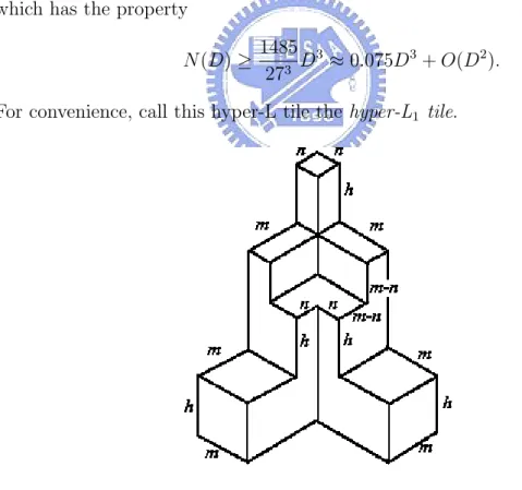
(11) 000 111 00 11 000 111 00 11 1 0 000 111 00 11 11 00 1 0 000 111 1 0 000 111 111 000 111 1 0 000 0 1 000 111 111 000 111 11 000 00 111 000 00 11 000 111 000 111 111 000 111 000 11 00 000 111 00 11 000 111 111 000 111 000 00 11 000111 111 000 m. m. l. n. n. Figure 3: A hyper-L tile.. Also, Aguiló-Gost [1] presented a new type of hyper-L tiles which is characterized by three parameters h, m, n, and is also highly structured and symmetrical (see Figure 4). Aguiló-Gost [1] used it to derive a new dense family of triple-loop networks which has the property N (D) ≥. 1485 3 D ≈ 0.075D3 + O(D2 ). 3 27. For convenience, call this hyper-L tile the hyper-L1 tile.. Figure 4: A hyper-L1 tile. While the hyper-L and the hyper-L1 tiles seem to be promising tools for studying the triple-loop network, we must be able to verify that those hyper-L tiles producing 4.

(12) good results are indeed the MDDs of some triple-loop networks. In [7], Chen et. al. have presented necessary and sufficient conditions for the existence of hyper-L triple-loop networks; see also [3]. In this thesis, we first prove that there exists a family of double-loop networks such that the sieve method requires Ω((log N )3/2 ) time to find the steps for each double-loop network in this family. We then propose a simple O(log N )-time algorithm to find the steps of a double-loop network with N nodes. We also give necessary and sufficient conditions for the existence of hyper-L1 triple-loop networks. This thesis is organized as follows: In Section 2, we briefly describe the Smith normalization method, the sieve method, and the CCH algorithm. In Section 3, we propose a simple O(log N )-time algorithm to find the steps of a double-loop network with N nodes. In Section 4, we give necessary and sufficient conditions for the existence of hyper-L1 triple-loop networks.. 2. The Smith normalization method, the sieve method, and the CCH algorithm. For completeness of this thesis, we briefly describe the Smith normalization method, the sieve method, and the CCH algorithm in this section. The sieve method is based on the sieve method in number theory and is very simple and easy to implement. The CCH algorithm is based on the Smith normalization method of Aguiló, Esqué and Fiol [2, 11], but unlike the Smith normalization method, it does not require any matrix operations and thus greatly simplifies the computation of the Smith normalization method. Given an L-shape, Aguiló and Fiol [2], and also Esqué et al. [11] proposed the following method for computing s1 and s2 such that DL(N ; s1 , s2 ) realizes L. THE-SMITH-NORMALIZATION-METHOD [2, 11]. Input: l, h, p, n of an L-shape L, where l > n, h ≥ p, and gcd(l, h, p, n) = 1. 5.

(13) Output: s1 and s2 such that DL(N ; s1 , s2 ) realizes the L-shape L(l, h, p, n). 1. Let. µ M=. l −p −n h. ¶ ,. M0 = M, i = 0, j = 0, k = 0. 2. Repeat the sub-steps 2.1-2.2 until the (1,1) element of Mj divides both the (2,1) element and the (1,2) element of Mj . 2.1 If the (1,1) element of Mj does not divide the (2,1) element of Mj , then let i = i + 1, j = j + 1, and find a nonsingular unimodular (i.e., determinant ± 1) integral matrix Li such that the (1,1) element of Mj = Li Mj−1 is the greatest common divisor of the first column of Mj−1 . 2.2 If the (1,1) element of Mj does not divide the (1,2) element of Mj , then let j = j + 1, k = k + 1, and find a nonsingular unimodular integral matrix Rk such that the (1,1) element of Mj = Mj−1 Rk is the greatest common divisor of the first row of Mj−1 . 3. If the (2,1) element of Mj is not zero, then let i = i + 1, j = j + 1, and find a nonsingular unimodular integral matrix Li to make the (2,1) element of Mj = Li Mj−1 zero. 4. If the (1,2) element of Mj is not zero, then let j = j + 1, k = k + 1, and find a nonsingular unimodular integral matrix Rk to make the (1,2) element of Mj = Mj−1 Rk zero. 5. If the (1,1) element of Mj does not divide the (2,2) element of Mj , then add column 2 of Mj to column 1 of Mj and go to Step 2. 6. Now Mj is the Smith normal form of M, i.e., µ Mj = Li · · · L2 L1 MR1 R2 · · · Rk = S(M) = 6. 1 0 0 N. ¶ ..

(14) Let L = Li · · · L2 L1 . If. µ L=. α β γ δ. ¶ ,. then let s1 = γ (mod N ) and let s2 = δ (mod N ). Return s1 , s2 .. Given an L-shape, Chen and Hwang [6] (see also [15]) proposed the following method, which is based on the sieve method in number theory, for computing s1 and s2 such that DL(N ; s1 , s2 ) realizes L. THE-SIEVE-METHOD [6]. Input: l, h, p, n of an L-shape L, where l > n, h ≥ p, and gcd(l, h, p, n) = 1. Output: s1 and s2 such that DL(N ; s1 , s2 ) realizes the L-shape L(l, h, p, n). 1. Let k = 0 and let F = the set of prime factors of N . 2. Let ak = kn + h, bk = kl + p, Fk = the set of prime factors of gcd(ak , bk ). 3. If f 6∈ Fk for all f ∈ F , then s1 = ak (mod N ) and s2 = bk (mod N ) realize L; otherwise, if f ∈ Fk for any f ∈ F , then go to Step 2.. We now prove that there exists a family of double-loop networks such that the sieve method requires Ω((log N )3/2 ) time to find the steps for each double-loop network in this family. The following lemma will be used in the proof. Lemma 1 Let p1 , p2 , · · · , pt be the smallest t primes, where t ≥ 2 and p1 < p2 < √ · · · < pt . If N = p1 × p2 × · · · × pt , then pt ≥ log N .. 7.

(15) Proof. Suppose N = p1 × p2 × · · · × pt . Then N ≤ (pt )! ≤ ppt t . Therefore log N ≤ pt log pt and log log N ≤ log pt + log log pt ≤ 2 log pt . So log pt ≥ √ √ log log N and we have pt ≥ log N .. 1 2. log log N =. Theorem 2 There exists a family of double-loop networks such that the sieve method requires Ω((log N )3/2 ) time to find the steps for each double-loop network in this family. Proof. Let t be an integer such that 2 ≤ t ≤ 100000. Let p1 , p2 , · · · , pt be the smallest t primes and p1 < p2 < · · · < pt . Let d = p1 × p2 × · · · × pt−1 . It is not difficult to verify that for each t in {2, 3, · · · , 100000}, pt ≤ 2pt−1 and thus j k l m j k 2d 2d are two consecutive integers. ≥ 1. Since 2d is not divisible by pt , pt and 2d pt pt Therefore » (2.2). ¼ ¹ º 2d 2d =1 − pt pt. and ¼ ¹ º 2d 2d ) = 1. , gcd ( pt pt. ». (2.3) Let. » l = pt. ¼ ¹ º 2d 2d − d. − d, h = d, p = d, n = pt pt pt. We claim that there exists a DL(N ; s1 , s2 ) realizing the L-shape(l, h, p, n). To prove this claim, we have to show that l > 0, h > 0, p ≥ 0, n ≥ 0, l ≥ p, h ≥ n, lh − pn = N, ³ ´ −d = and to show that the three conditions in (1.1) hold. It is clear that l > pt 2d pt ´ ³ j k − 1 − d ≥ 0. We ≥ 1, we have n > pt 2d d > 0, h = d > 0, p = d ≥ 0. Since 2d pt pt have l ≥ p since. » l = pt. ¼ µ ¶ 2d 2d − d = d = p. − d ≥ pt pt pt 8.

(16) We have h ≥ n since µ h = d = pt. 2d pt. ¶. ¹ − d ≥ pt. º 2d − d = n. pt. Let N = p1 × p2 × · · · × pt . Then ¶ ¶ µ ¹ º µ » ¼ 2d 2d −d − d d − d pt lh − pn = pt pt pt µ» ¼ ¹ º¶ 2d 2d − = dpt pt pt = dpt. (by (2.2)). = N. By (2.2), we have l > n. Since h = p, we have h ≥ p. Note that (2.4). gcd(pt , d) = gcd(pt , p1 × p2 × · · · × pt−1 ) = 1.. Thus ¼ ¹ º 2d 2d − d) − d, d, d, pt gcd (l, h, p, n) = gcd (pt pt pt ¹ º » ¼ 2d 2d , d) , pt = gcd (pt pt pt » ¼ ¹ º 2d 2d , d) (by (2.4)) , = gcd ( pt pt. ». = 1. (by (2.3)) We now claim that for each t in {2, 3, · · · , 100000}, the sieve method requires Ω((log N )3/2 ) time to find the steps for each double-loop network with L-shape L(l, h, p, n). Since N = p1 × p2 × · · · × pt , in the sieve method we will have F = {p1 , p2 , · · · , pt }. Since gcd(a0 , b0 ) = gcd(h, p) = d, we have F0 = {p1 , p2 , . . . , pt−1 }. 9.

(17) l m j k 2d − d + d) = − d + d, p Since gcd(a1 , b1 ) = gcd(n + h, l + p) = gcd(pt 2d t pt pt l m j k ), by (2.3) we have gcd(a1 , b1 ) = pt and therefore , pt 2d gcd(pt 2d pt pt F1 = {pt }. Recall that p1 , p2 , · · · , pt are the smallest t primes and p1 < p2 < · · · < pt ; i.e., p1 = 2, p2 = 3, p3 = 5, · · · . Note that if f ∈ F appears in Fk for some k and kf is the smallest such k, then f appears in every f th k after kf . Therefore p1 ∈ F appears in gcd(a0 , b0 ), gcd(a2 , b2 ), gcd(a4 , b4 ), gcd(a6 , b6 ), etc, p2 ∈ F appears in gcd(a0 , b0 ), gcd(a3 , b3 ), gcd(a6 , b6 ), gcd(a9 , b9 ), etc, p3 ∈ F appears in gcd(a0 , b0 ), gcd(a5 , b5 ), gcd(a10 , b10 ), gcd(a15 , b15 ), etc, p4 ∈ F appears in gcd(a0 , b0 ), gcd(a7 , b7 ), gcd(a14 , b14 ), gcd(a21 , b21 ), etc, ··· pt−1 ∈ F appears in gcd(a0 , b0 ), gcd(apt−1 , bpt−1 ), gcd(apt−1 ×2 , bpt−1 ×2 ), etc, pt ∈ F appears in gcd(a1 , b1 ), gcd(apt +1 , bpt +1 ), gcd(apt ×2+1 , bpt ×2+1 ), , etc. Thus the first k such that f 6∈ Fk for all f ∈ F is pt . By Lemma 1, pt ≥. √. log N .. Since each iteration of the sieve method involves the Euclidean algorithm, the sieve method requires Ω((log N )3/2 ) time and we have this theorem. We now describe the CCH algorithm. Given an L-shape L, Chan, Chen and Hong [5] proposed the following algorithm for computing s1 and s2 such that DL(N ; s1 , s2 ) realizes L. For completeness, we append the proof of the correctness of the CCH algorithm in the appendix.. The CCH algorithm [5]. Input: l, h, p, n of an L-shape L, where l > n, h ≥ p, and gcd(l, h, p, n) = 1. Output: s1 and s2 such that DL(N ; s1 , s2 ) realizes L. 10.

(18) 1. Find r1 = gcd(l, −n). 2. Find integers α1 and β1 such that α1 l + β1 (−n) = r1 . 3. Find r2 = gcd(r1 , −α1 p + β1 h). 4. Find integers α2 and β2 such that α2 r1 +β2 (−α1 p+β1 h) = r2 and gcd(β2 , r2 ) = 1. 5. s1 = α2 n − β2 h (mod N ) and s2 = α2 l − β2 p (mod N ).. In [5], Step 4 is performed by the following algorithm. ALGORITHM-MODIFIED-EUCLIDEAN [5]. Input: Integers a and b, not both zero, and r = gcd(a, b). Output: Integers x and y such that xa + yb = r and gcd(y, r) = 1. 1. Find integers α and β such that αa + βb = r. 2. If gcd(β, r) = 1, then let x = α, y = β, return x, y and stop this algorithm. 3. Let k = gcd(β, r), r0 = r, and d = k. 4. WHILE (d > 1) DO BEGIN r0 = r0 /d; d = gcd(r0 , k); END 5. Let a0 = a/r, b0 = b/r, x = α + r0 b0 and y = β − r0 a0 . Return x, y.. For example, let l = 5, h = 3, p = 3, and n = 2. Then the CCH algorithm derives r1 = 1, α1 = 1, β1 = 2, r2 = 1, α2 = −2, and β2 = 1. 11.

(19) Thus N = 9, s1 = −7 (mod 9) = 2, and s2 = −13. (mod 9) = 5.. It can be verified from Figure 2 that DL(9; 2, 5) realizes L-shape(5,3,3,2).. 3. Our algorithm. Our algorithm is based on the CCH algorithm and therefore unlike the Smith normalization method, our algorithm does not require any matrix operations. It is well-known that Lemma 3 If a and b are integers, not both zero, then there exist integers α and β such that αa + βb = gcd(a, b). It is known that gcd(a, b) = gcd(|a|, |b|) and if |b| ≥ |a| > 0, then α, β, and gcd(a, b) can be found in O(log |a|) time by using the Euclidean algorithm [9]. Chan et. al. [5] proved that Lemma 4 [5] If α, a, β, b are integers, not all zero, such that αa + βb = 1, then gcd(a, β) = 1. Step 4 of the CCH algorithm is based on Theorem 5 described below. Theorem 5 [5] If a and b are integers, not both zero, then there exist integers x and y such that xa + yb = gcd(a, b) and gcd(y, gcd(a, b)) = 1. Recall that N = lh − pn. It is obvious that Steps 1, 2, and 3 of the CCH algorithm can be done in O(log N ) time by using the Euclidean algorithm. Step 5 of the CCH algorithm takes O(1) time. Since Step 4 of the CCH algorithm takes O((log N )2 ) time (see [5] for details), the CCH algorithm takes O((log N )2 ) time. We thus conclude that if Step 4 of the CCH algorithm can be done in O(log N ) time, then the CCH algorithm takes only O(log N ) time and the steps of a doubleloop network with N nodes can be found in O(log N ) time. The key observation of 12.

(20) our algorithm is that Theorem 5 can be proved in another way and this new proof leads to an O(log N )-time implementation for Step 4 of the CCH algorithm. A new proof for Theorem 5. Set r = gcd(a, b) for easy writing. By Lemma 3, there exist integers α and β such that αa + βb = r. If gcd(β, r) = 1, then we are done. In the following, assume that gcd(β, r) = k > 1. Let r0 be the largest integer such that (3.5). r0 | r and gcd(r0 , k) = 1.. Then either r0 = 1 or r0 > 1. In the former case, every prime factor of r is also a prime factor of k. In the latter case, every prime factor of r is either a prime factor of k or a prime factor of r0 . Let a0 = a/r, and b0 = b/r. Note that gcd(r0 , β) = 1; otherwise, we will have gcd(β, r) > k. Since αa + βb = r, we have αa0 + βb0 = 1. By Lemma 4, we have gcd(a0 , β) = 1. Since gcd(a0 , β) = 1 and k | β, we have gcd(a0 , k) = 1. Since k | β and gcd(r0 , k) = 1 and gcd(a0 , k) = 1, we have (3.6). gcd(β − r0 a0 , k) = 1.. Since gcd(r0 , β) = 1 and r0 | r0 a0 , we have (3.7). gcd(β − r0 a0 , r0 ) = 1.. Recall that r0 = 1 or r0 > 1. In the former case, by (3.6), by (3.7), and by the fact that every prime factor of r is also a prime factor of k, we have gcd(β − r0 a0 , r) = 1. 13.

(21) In the latter case, by (3.6), by (3.7), and by the fact that every prime factor of r is either a prime factor of k or a prime factor of r0 , we also have gcd(β − r0 a0 , r) = 1. Let x = α + r0 b0 and y = β − r0 a0 .. (3.8) Then. xa + yb = (α + r0 b0 )a + (β − r0 a0 )b = r and gcd(y, r) = gcd(β − r0 a0 , r) = 1. We proved the theorem. The following lemma provides an efficient way to find r0 in (3.8), which is the largest integer satisfying (3.5). Lemma 6 Let r and k be positive integers such that k | r and k > 1. Then r0 =. r gcd(k blog2 rc , r). is the largest integer satisfying (3.5). Proof. Assume that k = ps11 ps22 · · · psmm , where p0i s are distinct prime factors of k. Also assume that t. t. m+1 m+2 r = pt11 pt22 · · · ptmm pm+1 pm+2 · · · ptnn ,. where p0j s are distinct prime factors of r. Note that when pm+1 , pm+2 , · · · , pn do not exist (this case occurs when k contains every prime factor of r), we will simple say t. t. m+1 m+2 that pm+1 pm+2 · · · ptnn = 1. It is clear that the largest integer satisfying (3.5) is. t. t. m+1 m+2 r0 = pm+1 pm+2 · · · ptnn. 14.

(22) and it suffices to prove that r. t. gcd(k blog2 rc , r). t. m+1 m+2 = pm+1 pm+2 · · · ptnn .. Note that blog2 rcs1 blog2 rcs2 p2. k blog2 rc = p1. blog2 rcsm · · · pm .. Since 2 is the smallest prime, we have ti ≤ blog2 rc, for all i, 1 ≤ i ≤ n. Therefore ti ≤ blog2 rcsi , for all i, 1 ≤ i ≤ m. Thus gcd(k blog2 rc , r) = pt11 pt22 · · · ptmm . So r gcd(k blog2 rc , r). t. =. t. m+1 m+2 pt11 pt22 · · · ptmm pm+1 pm+2 · · · ptnn tm+1 tm+2 = pm+1 pm+2 · · · ptnn . t1 t2 t m p1 p2 · · · pm. The new proof of Theorem 5 and Lemma 6 lead to the following new algorithm for finding x and y in Theorem 5. ALGORITHM-NEW-MODIFIED-EUCLIDEAN. Input: Integers a and b, not both zero, and r = gcd(a, b). Output: Integers x and y such that xa + yb = r and gcd(y, r) = 1. 1. Find integers α and β such that αa + βb = r. 2. Find k = gcd(β, r). 3. If k = 1, then let x = α, y = β, return x, y and stop this algorithm.. 15.

(23) 4. If k ≥ 2 , find r0 =. r gcd(k blog2 rc , r). .. 5. Let a0 = a/r, b0 = b/r, x = α + r0 b0 and y = β − r0 a0 . Return x, y.. The correctness of ALGORITHM-NEW-MODIFIED-EUCLIDEAN follows from Lemma 6. We now prove that: Theorem 7 If we use ALGORITHM-NEW-MODIFIED-EUCLIDEAN instead of ALGO RITHM-MODIFIED-EUCLIDEAN in Step 4 of the CCH algorithm, then the CCH algorithm takes O(log N ) time to find the steps of a double-loop network. Proof. Recall that N = lh − pn. Since Steps 1, 2, 3, and 5 of the CCH algorithm take O(log N ) time, it suffices to prove that ALGORITHM-NEW-MODIFIEDEUCLIDEAN takes O(log N ) time. When Step 4 of the CCH algorithm is performed, inputs to ALGORITHM-NEW-MODIFIED-EUCLIDEAN are a = r1 , b = −α1 p + β1 h, r = gcd(r1 , −α1 p + β1 h). In the following, Step i refers to Step i in ALGORITHM-NEW-MODIFIED-EUCLIDEAN. Since r1 = gcd(l, −n), we have r1 > 0, r1 ≤ N, and min{|a|, |b|} = min{|r1 |, | − α1 p + β1 h|} ≤ |r1 | = r1 ≤ N. Therefore Step 1 can be done in O(log N ) time by using the Euclidean algorithm. Since r = gcd(r1 , −α1 p + β1 h), we have r > 0, r ≤ r1 ≤ N, 16.

(24) and min{|β|, |r|} ≤ |r| = r ≤ N. Therefore, in Step 2, finding k = gcd(β, r) can be done in O(log N ) time by using the Euclidean algorithm. It is obvious that Step 3 and Step 5 can be done in O(1) time. It remains to prove that in Step 4, finding r0 =. r gcd(kblog2 rc ,r). can also be done. in O(log N ) time. Note that computing k blog2 rc takes O(logblog2 rc) = O(log log N ) time. Since r > 0 and r ≤ N , we have min{|k blog2 rc |, |r|} ≤ |r| = r ≤ N. Therefore, finding gcd(k blog2 rc , r) takes O(log r) = O(log N ) time. Hence finding r0 =. r gcd(kblog2 rc ,r). takes a total O(log log N ) + O(log N ) + 1 = O(log N ). time, where +1 is for the division. From the above, Step 4 can be done in O(log N ) time. We have this theorem.. 4. Necessary and sufficient conditions for the existence of hyper-L1 triple-loop networks. The following two lemmas will be used in the remaining discussions. Lemma 8 If a, m, b, n are integers, not all zero, such that am − bn = 1, then gcd(a, n) = 1. Proof. Assume that am − bn = 1 and gcd(a, n) = k. Then k | a and k | n. Thus k | am − bn = 1. So k = 1.. Lemma 9 If m and n are integers, not both zero, and gcd(m, n) = 1, then there exist integers a and b such that am − bn = 1 and gcd(a, 2m + n) = 1.. 17.

(25) Proof. By Lemma 3, there exist integers a and b such that am − bn = 1. By Lemma 8, we have (4.9). gcd(a, n) = 1.. If gcd(a, 2m + n) = 1, then we are done. In the following, assume that gcd(a, 2m + n) = d > 1. Let a = pd and 2m + n = qd. Then gcd(p, q) = 1. Since gcd(m, n) = 1, we have ½ 1 if n is odd, gcd(2m + n, n) = gcd(2m, n) = 2 if n is even. If gcd(2m + n, n) = 1, then clearly gcd(qd, n) = 1 and thus gcd(d, n) = 1. Now suppose that gcd(2m + n, n) = 2. Then gcd(qd, n) = 2; therefore gcd(d, n) = 1 or gcd(d, n) = 2. If gcd(d, n) = 2, then 2 | a and we have gcd(a, n) ≥ 2; this contradicts with(4.9). From the above, we have (4.10). gcd(d, n) = 1.. Let q = st, where s is the largest factor of q such that (4.11). gcd(s, d) = 1.. That is, s (t) contains those prime factors of q that are relative prime (not relative prime) to d. (As an example, if q = 22 ·32 ·7 and d = 2·32 , then s = 7 and t = 22 ·32 .) Then (4.12). gcd(s, t) = 1.. Since gcd(p, q) = 1 and q = st, we have (4.13). gcd(p, s) = 1. 18.

(26) Since t contains those prime factors of q that are not relative prime to d, by (4.10), we have (4.14). gcd(t, n) = 1.. Let a0 = a + sn and b0 = b + sm. Then a0 m − b0 n = (a + sn)m − (a + sm)n = am − bn = 1. Moreover, gcd(a0 , 2m + n) = gcd(a + sn, 2m + m) = gcd(pd + sn, qd) = gcd(pd + sn, q) (by (4.10) and (4.11)) = gcd(pd + sn, st) = gcd(pd + sn, s) (by (4.12) and (4.14)) = 1 (by (4.11) and (4.13)). Thus we have this lemma. Let HL1 (h, m, n) denote a hyper-L1 tile with parameters h, m, n. Aguiló-Gost [1] defined  n −m −m M1 (h, m, n) =  n n + m −m  2h h 2h − n . and derived that the diameter of HL1 (h, m, n) is given by (4.15). D(h, m, n) = max{3m + h + n, 2m + 2h + n, 3h + 3n} − 3.. Note that two sides labelled length n in Figure 5 in [1] are actually of length m − n; see Figure 5 This flaw can be verified by checking the lengths of the sides 19.

(27) of the topmost n × n square and the lengths of the sides of the rightmost m × h rectangle. See Figure 4 for a correction of Figure 5. Thus matrix M1 should be  n −m −m  −m M1 (h, m, n) =  n n + m 2h h h+m−n . and the diameter of HL1 (h, m, n) should be (4.16). D(h, m, n) = max{3m + h + n, 2m + 2h + n, 3h + 3n, m + 2h + 3n} − 3.. Figure 5: The Fig. 5 in [1]. Note that the difference between the diameters derived by (4.15) and by (4.16) can be quite large. To see this, let h = 2t − 1 − k m = 2t − 1 n = t + k, where t and k are positive integers chosen in such a way that both gcd(m, n) = 1 and 3 - m − n are satisfied. Then the diameter derived by (4.15) is 9t − 6, while the. 20.

(28) diameter derived by (4.16) is 9t − 6 + k. The difference between the two diameters is k. As an example, when k = 5, we can choose t = 10, h = 14, m = 19, and n = 15. Aguiló-Gost [1] observed that HL1 (h, m, n) tessellates the space. By studying the distribution of node 0 in the space, Aguiló-Gost obtained     0 s1 M T ×  s2  ≡  0  (mod N ) or 0 s3    α s1 T    β  N for some integers α, β, γ. s2 = M × γ s3 . (4.17). Also, N = det M . For convenience, we call a triple-loop network whose MDD is HL1 (h, m, n) an HL1 (h, m, n) triple-loop. We now give a necessary and sufficient condition for the existence of an HL1 (h, m, n) triple-loop. Theorem 10 A necessary and sufficient condition for the existence of an HL1 (h, m, n) triple-loop is gcd(m, n) = 1 and 3 - m − n. Proof. Note that N = det M . Suppose an HL1 (h, m, n) triple-loop exists. From (4.17), we have   s1  s2  s3   α ¡ T ¢−1  β N = M γ    h(2m + n) + (m − n)(m + n) −(h(2m + n) + n(m − n)) −h(2m + n) α    m(m − n) h(2m + n) + n(m − n) −h(2m + n) β . = m(2m + n) 0 n(2m + n) γ Suppose that gcd(m, n) = 1 and 3 - m − n. Since gcd(m, n) = 1, by Lemma 9, there exist integers a and b such that am − bn = 1 and gcd(a, 2m + n) = 1. Since gcd(a, 2m + n) = 1, we have a 6= 0. Since gcd(m, n) = 1, gcd(m − n, m) = 1. 21.

(29) Since gcd(m, n) = 1, 3 - m − n, and gcd(m − n, m) = 1, (4.18). gcd(m − n, 2m + n) = gcd(m − n, 3m) = gcd(m − n, 3) = 1.. Setting (α, β, γ) = (a, 0, −b), we obtain the solution     h(a + b)(2m + n) + a(m − n)(m + n) (mod N ) s1 .  s2  =  bh(2m + n) + am(m − n) (mod N ) 2m + n s3 Since N = det M , we have (4.19). N = (2m + n)(h(2m + n) + n(m − n)).. Let. ½ φ(a) =. −1 1. if a > 0, if a < 0.. From (4.19), 2m + n | N . Since 2m + n | N , there exists an integer k1 such that h(a + b)(2m + n) + a(m − n)(m + n). (mod N ). = k1 (2m + n) + φ(a)a(m − n)(m + n) and 0 < k1 (2m + n) + φ(a)a(m − n)(m + n) < N . Also, there exists an integer k2 such that bh(2m + n) + am(m − n). (mod N ). = k2 (2m + n) + φ(a)am(m − n) and 0 < k2 (2m + n) + φ(a)am(m − n) < N . Therefore     k1 (2m + n) + φ(a)a(m − n)(m + n) s1 .  s2  =  k2 (2m + n) + φ(a)am(m − n) 2m + n s3. 22.

(30) Note that gcd(k1 (2m + n) + φ(a)a(m − n)(m + n), k2 (2m + n) + φ(a)am(m − n), 2m + n) = gcd(a(m − n)(m + n), am(m − n), 2m + n) = gcd(an(m − n), am(m − n), 2m + n) = gcd(n(m − n), m(m − n), 2m + n) (by the fact that gcd(a, 2m + n) = 1) = gcd(n, m, 2m + n) (by (4.18)) = gcd(m, n) = 1. So if gcd(m, n) = 1 and 3 - m − n, then clearly gcd(N, s1 , s2 , s3 ) = gcd(s1 , s2 , s3 ) = 1 and T L(N ; s1 , s2 , s3 ) exists. On the other hand, suppose gcd(m, n) = d > 1 or 3 | m − n. In the former case, each si , i = 1, 2, 3, is a linear combination of terms divisible by d. Furthermore, from (4.19), N is also a linear combination of terms divisible by d. Hence gcd(N, s1 , s2 , s3 ) ≥ d > 1 and T L(N ; s1 , s2 , s3 ) does not exist. In the latter case, since 3 | m − n, we have gcd(2m + n, m − n) = gcd(3m, m − n) = r ≥ 3. Therefore each si , i = 1, 2, 3, is a linear combination of terms divisible by r. Furthermore, from (4.19), N is also a linear combination of terms divisible by r. Hence gcd(N, s1 , s2 , s3 ) ≥ r > 1 and T L(N ; s1 , s2 , s3 ) does not exist.. 23.

(31) References [1] F. Aguiló-Gost, New dense families of triple loop networks, Disc. Math. 197/198 (1999) 15-27. [2] F. Aguiló and M. A. Fiol, An efficient algorithm to find optimal double loop networks, Disc. Math. 138 (1995), 15-29. [3] F. Aguiló, M. A. Fiol and C. Garcia, Triple-loop networks with small transmission delay, Disc. Math. 167/168 (1997) 3-16. [4] J.-C. Bermond, F. Comellas and D. F. Hsu, Distributed loop computer networks: a survey, J. Parallel Distribut. Comput. 24 (1995), 2-10. [5] R. C. Chan, C. Y. Chen and Z. X. Hong, A simple algorithm to find the steps of double-loop networks, Disc. Appl. Math. 121 (2002), 61-72. [6] C. Y. Chen and F. K. Hwang, The minimum distance diagram of double-loop networks, IEEE Trans. Comput. 49 (2000), 977-979. [7] C. Y. Chen, F. K. Hwang, J. S. Lee and S. J. Shih, The existence of hyper-L triple-loop networks, Disc. Math. 268 (2003) 287-291. [8] Y. Cheng and F. K. Hwang, Diameters of weighted double loop networks, J. Algorithms 9 (1988), 401-410. [9] T. H. Cormen, C. E. Leiserson, R. L. Rivest, and C. Stein, Introduction to Algorithms, 2nd Ed. (2001), The MIT Press, 856-862. [10] P. Erdös and D. F. Hsu, Distributed loop networks with minimum transmission delay, Theoret. Comput. Sci. 100 (1992), 223-241. [11] P. Esqué, F. Aguiló, and M. A. Fiol, Double commutative-step diagraphs with minimum diameters, Disc. Math. 114 (1993), 147-157.. 24.

(32) [12] M. A. Fiol, M. Valero, J. L. A. Yebra, I. Alegre, and T. Lang, Optimization of double-loop structures for local networks, in Proc. XIX Int. Symp. MIMI’82, Paris, France (1982), 37-41. [13] M. A. Fiol, J. L. A. Yebra, I. Alegre, and M. Valero, A discrete optimization problem in local networks and data alignment, IEEE Trans. Comput. C-36 (1987), 702-713. [14] F. K. Hwang, A survey on double-loop networks, Reliability of Computer and Communication Networks, Eds: F. Roberts, F. K. Hwang and C. Monma, AMS series (1991), 143-151. [15] F. K. Hwang, A complementary survey on double-loop networks, Theoret. Comput. Sci. A 263 (2001), 211-229. [16] F. K. Hwang, A survey on multi-loop networks, Theoret. Comput. Sci. A 299 (2003), 107-121. [17] F. K. Hwang and Y. H. Xu, Double loop networks with minimum delay, Disc. Math. 66 (1987), 109-118. [18] J. M. Peha and F. A. Tobagi, Analyzing the fault tolerance of double-loop networks, IEEE Trans. Network. 2 (1994), 363-373. [19] C. K. Wong and D. Coppersmith, A combinatorial problem related to multimodule memory organizations, J. Assoc. Comput. Mach. 21 (1974), 392-402.. 25.

(33) Appendix Theorem 11 [5] The CCH algorithm is correct and it takes at most O((log N )2 ) time. Proof. Note that N = lh − pn. Let µ M=. l −p −n h. ¶. Consider column 1 of M: it contains l and −n. After Step 1 is performed, we have r1 = gcd(l, −n) and α1 l + β1 (−n) = r1 . Let ¶ µ α1 β1 . L1 = l n r1. r1. and let M1 = L1 M. Then ¶ ¶µ ¶ µ µ α1 β1 r1 −α1 p + β1 h l −p . = M1 = N l n 0 −n h r1 r1 r1 Consider row 1 of M1 : it contains r1 and −α1 p + β1 h. After Step 2 is performed, we have r2 = gcd(r1 , −α1 p + β1 h), α2 r1 + β2 (−α1 p + β1 h) = r2 , and gcd(β2 , r2 ) = 1. Let. Ã R1 =. α2 β2. −(−α1 p+β1 h) r2 r1 r2. and let M2 = M1 R1 . Then ¶Ã µ r1 −α1 p + β1 h α2 M2 = N 0 β2 r1. !. −(−α1 p+β1 h) r2 r1 r2. Consider column 1 of M2 : it contains r2 and. N β2 . r1. .. !. µ =. r2. N β2 r1. 0. ¶. N r2. .. ). Note Let r3 = gcd(r2 , Nrβ2 1. that in Step 2 we choose gcd(β2 , r2 ) = 1. Thus ) = gcd(r2 , rN1 ) = gcd(r1 , −α1 p + β1 h, rN1 ). r3 = gcd(r2 , Nrβ2 1 We claim that r3 = 1. Suppose this is not true and r3 > 1. Then every entry of M1 is a multiple of r3 . Since M1 = L1 M, we have ¶ ¶µ µ l −β 1 r −α p + β h 1 1 1 1 −1 r1 . M = L1 M1 = N 0 det(L1 ) − rn1 α1 r1 26.

(34) That is, 1 M= det(L1 ). µ. l r1 − rn1. −β1 α1. ¶. µ. r1 r3. r3. 0. −α1 p+β1 h r3 N r1 r3. ¶ .. Since r3 = gcd(r1 , −α1 p + β1 h, rN1 ), µ. −α1 p+β1 h r3 N r1 r3. r1 r3. 0. ¶. is integral. Since det(L1 ) = ±1, every entry of M must be a multiple of r3 . Then gcd(l, h, p, n) ≥ r3 > 1; this contradicts with the assumption that gcd(l, h, p, n) = 1. Therefore r3 = 1. ) and r3 = 1, by Lemma 3, there exist integers α3 and β3 Since r3 = gcd(r2 , Nrβ2 1 such that α3 r2 + β3 ( Nrβ1 2 ) = 1. Let µ L2 =. α3. β3 r2. r2. 0. −N β2 r1. ¶ .. and let M3 = L2 M2 . Then µ M3 =. α3. β3 r2. −N β2 r1. ¶µ. N β2 r1. Let. µ R2 =. ¶ =. N r2. 1 − βr32N 0 1. µ. 1 0. β3 N r2. ¶ .. N. ¶ .. and let M4 = M3 R2 . Then µ M4 =. 1 0. β3 N r2. ¶µ. N. 1 − βr32N 0 1. ¶. µ =. 1 0 0 N. ¶ = S(M).. From the above, L2 L1 MR1 R2 = S(M). Moreover, L1 , L2 , R1 and R2 are unimodular integral matrices. Let L = L1 L2 . Then ! ¶ Ã ¶µ µ α3 α1 + βr11n α3 β1 + βr31l α3 β3 α1 β1 . = L= −N β2 l n −N β2 β1 +r2 l −N β2 α1 +r2 n r2 r1 r1 r1 r r 1. 1. Using the facts that N = lh − pn and α1 l + β1 (−n) = r1 and α2 r1 + β2 (−α1 p + β1 h) = r2 , we have. −N β2 α1 +r2 n r1. = α2 n − β2 h and. −N β2 β1 +r2 l r1. = α2 l − β2 p. Thus if. S1 = α2 n − β2 h (mod N ) and s2 = α2 l − β2 p (mod N ), then DL(N ; s1 , s2 ) realizes L. 27.

(35) It is clear that Steps 1, 2, and 3 can be done in O(log N ) time by using the Euclidean algorithm. Step 4 can be done in O((log N )2 ) time by using ALGORITHMMODIFIED-EUCLIDEAN. Step 5 can be done in O(1) time. Thus the CCH algorithm takes at most O((log N )2 ).. 28.

(36)