A Storage Management for Mining Object Moving Patterns in Object Tracking
Sensor Networks
Chih-Chieh Hung and Wen-Chih Peng
∗Department of Computer Science
National Chiao Tung University
Hsinchu, Taiwan, ROC
E-mail:{[email protected], [email protected]}
Abstract
One promising application of sensor networks is object tracking. Because the movements of the tracked objects usu-ally show repeating patterns, we propose a heterogeneous tracking model, referred to as HTM, to efficiently mine ob-ject moving patterns and track obob-jects. To ensure the qual-ity of moving patterns, we develop a storage management to facilitate mining object moving patterns. Specifically, we explore load-balance feature to store more moving data for mining moving patterns. Once a storage of a cluster head is occupied by moving data, we devise a replacement strategy to replace the less informative patterns. Simulation results show that HTM with storage management is able not only to increase the accuracy of predition but also to save more energy in tracking objects.
1 Introduction
Object tracking is one of the killer applications for wire-less sensor networks. Various energy conservation schemes for object tracking sensor networks have been extensively studied in the literature [3][5]. In this paper, we concen-trate at the prediction-based object tracking sensor network. The prediction-based object tracking sensor networks relies on certain prediction mechanisms to achieve energy saving. We argue that tracked objects such as human or animals tend to have their own moving patterns since the behaviors of human or animals are likely to be regular [4]. Thus, ef-ficient techniques for obtaining moving patterns of objects are very important for energy conservation in object track-ing sensor networks. Various data mintrack-ing techniques have been explored in the literature [1]. However, these prior works mostly require data to be collected at one central-ized server, leading to a significant amount of energy
con-∗The corresponding author of this paper.
sumption in data collection. Our goal is to propose an ef-ficient data mining mechanism for deriving object moving patterns in object tracking sensor network and utilize the object moving patterns for energy saving prediction-based object tracking sensor networks.
To facilitate collaborative data collection processing in object tracking sensor networks, cluster architectures are usually used to organize sensor nodes into clusters (with each cluster consisting of a cluster head and sensors). Sim-ilar to [2], we consider the sensor network which consists of heterogeneous nodes of various functions and roles and thus propose a heterogeneous tracking model (referred to as HTM) in the cluster architecture, in which a large number of inexpensive sensor nodes perform sensing operations and a limited number of heterogeneous nodes (standing for clus-ter heads) offer data collection and mining capabilities. For scalability, the cluster heads recursively form a hierarchical architecture for efficiently mining and queries. As such, the higher-level cluster heads will maintain coarse object mov-ing patterns and the low-level cluster heads will have more precise object moving patterns. Based on the obtained ob-ject moving patterns, the cluster heads predict the obob-ject movements. If the prediction fails, a recovery procedure will be executed by waking up sensor nodes within the cov-erage region of the cluster head. Based on HTM, only a bound number of sensor nodes need to participate in the re-covery procedure.
In HTM, cluster heads should keep as many moving log data as possible in their clusters. Note that cluster heads also have storage constraint and the amount of data will affect the effect of pattern mining. Notice that the conventional hierarchy clustering architectures (i.e., the level i cluster head is chosen among these level (i-1) cluster heads) suf-fer from the storage load unbalance problem. Assume that the storage space of a cluster head is S and the height of hierarchy is k, there is always a cluster head (called heavy node) which stores information of all level in the hierarchy
and thus can only useS
k to store information of each level.
The heavy node can only mine patterns with shorter term than these cluster heads that only store information of one or fewer levels. In this paper, we develop a storage manage-ment, which consists of two modules: load-balance storage scheme and one replacement strategy. In the load-balance scheme, we address how to mine and maintain the informa-tive patterns under the storage constraints of cluster heads. We develop a replace strategy to replace less informative patterns when the storage space of a cluster head is full.
The rest of the paper is organized as follows. Preliminary is described in Section 2. Storage management for HTM is presented in Section 3. Performance study is conducted in Section 4. This paper concludes with Section 5.
2 Preliminaries
In this section, we briefly illustrate the tracking mecha-nism used in HTM. Assume that low-end sensor nodes and cluster heads have unique sensor identifications and these sensor nodes are well time-synchronized. Suppose that each low-end sensor node is a logical representation of a set of sensor nodes which collaboratively detect an object. When a low-end sensor detects an object, this sensor node will in-form the corresponding level-0 cluster heads of the detected object identification, object arrival time and its sensor iden-tification. In other words, the location of an object is repre-sented as a sensor identification and the moving log for each object is viewed as a moving stream, which is composed of a series of symbols. Since the cluster heads still have the storage constraint, in this paper, we adopt the variable mem-ory Markov (referred to as VMM) model, which has been shown to be very effective in capturing dependences and in obtaining sequential models in one scan, to discover object moving behavior in every cluster head.
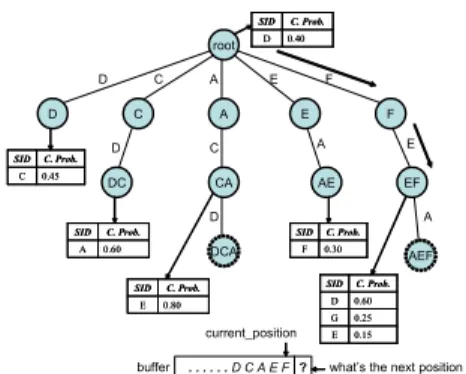
Due to the storage constraint in cluster head and the de-pendence of movements, mining object moving patterns can be regarded as a VMM model training. For each object, we use a variation of a suffix tree called emission tree [6] to maintain its VMM model and one corresponding buffer in a cluster head is used to hold the most recently segment of moving records. Each edge of an emission tree represents a moving record (i.e., sensor id) appearing in the moving path. A tree node of an emission tree is denoted as a con-catenation of the edge labels from the node to the root. In other words, a tree node labeled as rk...r2r1can be reached
from the traversal path from root → r1→ r2→ ... → rk.
Each tree node will maintains the occurrence number of its label in the moving path. Furthermore, each tree node also records the conditional probabilities of all consecutive mov-ing records given the node label as the precedmov-ing segment. For example, according to the conditional probabilities of consecutive moving records of node EF in Figure 1, it can
root D C DC A CA DCA E AE F EF AEF D C A E F D C D A E A 0.45 C C. Prob. SID 0.45 C C. Prob. SID 0.60 A C. Prob. SID 0.60 A C. Prob. SID 0.40 D C. Prob. SID 0.40 D C. Prob. SID 0.80 E C. Prob. SID 0.80 E C. Prob. SID 0.30 F C. Prob. SID 0.30 F C. Prob. SID 0.15 E 0.25 G 0.60 D C. Prob. SID 0.15 E 0.25 G 0.60 D C. Prob. SID . . . D C A E F ? buffer current_position
what’s the next position ?
Figure 1. The resulting emission tree. The nodes with dash circle are immature. Aother nodes are mature.
be verified that P(D|EF) is 0.60. Consequently, if the most recently moving record is EF, one can estimate the consec-utive movement to be D.
VMM model is trained on the fly and not all the tree nodes are suitable for predicting. There are two kind of nodes in an emission tree: mature node and immature node. Mature nodes are those tree nodes whose the conditional probabilities are stable. When predicting the next move-ment, only mature node is participated in prediction. Fol-lowing the above example, the mature node EF is used to predict instead of the immature node AEF. To justify whether a node is mature or not, we explore L∞ distance, which is defined as follows:
Definition 1: For a node y with the corresponding
proba-bility table denoted as x and the number of tuples in table x is n, L∞(x, x0) = max
i=1,...,n(|dxi − dx
0
i |), where dxi
rep-resents the probability value for tuple i in table x and table x0is the probability table after updating.
Definition 2: For node y and given two application
depen-dent parameters α and β, if L∞(x, x0) ≤ α for β times of
successive updates, then node y is a mature node.
3 Storage Management for HTM
Since the quality of moving patterns are the dominant factor for HTM, the storage management is thus an impor-tant issue for HTM. In Section 3.1, we develop a new stor-age scheme for HTM. In Section 3.2, we devise a replace-ment strategy to keep the most informative patterns when memory space of a cluster head is full.
3.1 Load-Balance Data Storage Scheme
To facilitate to understand the concept, we assume that cluster heads are grid deployed and the degree of
hierar-chy is four1. To avoid the heavy node problem of
conven-tional hierarchy architectures, we must consider the number of levels of information a cluster head stores. Once a clus-ter head stores too much information, we tend to separate data flows to other cluster heads stored fewer information. Based on this concept, we propose a storage load-balanced scheme for HTM:
Given child cluster heads Ciin level i and the coordinate
of sink, the parent cluster head of Ciis assigned by the
fol-lowing rules: If there exist a cluster head v ∈ Cisuch that
v stores only one level of information and v is the nearest sink among any cluster head u∈Ci, then v is parent cluster
head of Ci. Otherwise, redirect the task to a cluster head w,
where w is the cluster heads closet to sink among all 1-hop neighbors of Ci. The sink is assigned to be parent in highest
level
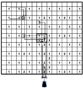
The proposed scheme can be illustrated as the following example. An illustrative example shows in Figure 2. Every square represents a cluster head. The square marked k is the cluster head stores the information of level 0 and level k. Sink is in the bottom of the network. Arrows repre-sent the data flow from low level cluster heads to its parent. Consider the circled level-2 cluster head, the circle level-2 cluster head in the marked region is the cluster head nearest to sink among circled level-2 cluster heads, but it already stores two levels of information and then redirects the task to its right neighbor. Its right neighbor stores only level 0 information and then become the parent of circled level-2 cluster heads.
To prove our scheme is storage load-balanced, we eval-uate the variance of storage cost. Suppose the height of the hierarchy is k, the expected value of the storage cost for each cluster head is EHT M = 4−4
−k
3 . Then we can
evalu-ate the variance of the storage cost as: VHT M = (2−EHT M)2(4k−13 )+(1−EHT M)2(2×4k +13 ) 4k = 2 9− 4−k 9 − 4−2k 9 = Θ(1)
Similarly, we can evaluate the storage cost for each clus-ter head using conventional clusclus-tering hierarchy architec-tures to be Θ(k2). It can be seen that V
HT M grows in the
constant rate and is independent to the height. Therefore we can conclude that the proposed scheme can satisfy the storage load-balance and thus ensure the quality of moving patterns for each cluster head.
3.2 Storage Replacement Strategy
Through the proposed storage scheme can ensure that a level i (i ≥ 1) cluster head only has to maintain two lev-els of information, with time passing by, the storage of each cluster head will run out. Therefore, we must to discard less
1That is, every parent cluster head in hierarhcy has four children.
1 1 2 1 1 2 1 1 2 1 1 2 3 1 1 1 1 3 1 1 1 1 2 1 1 2 1 1 2 1 1 2 1 1 1 1 1 1 3 1 1 1 1 2 3 2 1 1 2 1 1 1 1 2 1 1 1 1 1 1 1 1 1 1 2 1 1 2 1 1 2 1 1 2 1 1 1 1 1 1 1 1 1 1 1 1 2 1 1 2 1 1 2 1 1 2 3 1 1 1 1 3 1 1 1 1 2 1 1 2 1 1 2 1 1 2 1 1 1 1 1 1 3 1 1 1 1 2 3 2 1 1 2 1 1 1 1 2 1 1 1 1 1 1 1 1 1 1 2 1 1 2 1 1 2 1 1 2 1 1 1 1 1 1 1 1 1 1
Figure 2. Storage load-balanced scheme for HTM.
informative patterns to store more informative ones. Hence, the storage replacement strategy is necessary for dealing with this situation. When the memory space of a cluster head is full and the count of one symbol in the table main-tained by an emission tree node is larger than given thresh-old min_sup, we have to decide to prune other nodes so that the newborn node can be inserted into emission trees. We specify a threshold and if the prediction hit rate of the tree to which the newborn node belongs is already larger than , we can ignore the insertion since this emission tree already has higher prediction rates. Otherwise, we must select an appropriate node to be pruned from other trees. The prun-ing mechanism consists two steps:
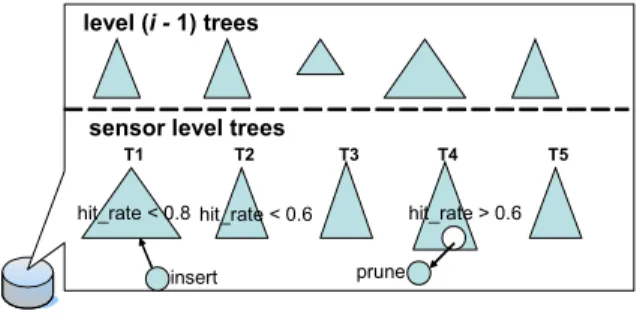
1) Select the tree to be pruned. Each object usually has its own moving behavior. An object may stay in some gions more frequently than other regions. Hence, the re-porting rates of objects in each cluster head will be differ-ent. For tree selection, each tree maintains a counter. The counter increases one when a tree is updated and minuses one every T periods. Obviously, a tree with a lower counter value means that it is not often used than other trees. Once a newborn generated, we only select the same level tree to the newborn node to prune. To guarantee that the accuracy of each tree is acceptable, we specify a threshold ξ. Sup-pose that the new node will be inserted into a level i emis-sion tree. Among other level i trees with their prediction hit rates ≥ ξ, the tree with the minimal counter value will be selected. Consider an example in Figure 3, where the size of a tree stands for the access counter value of the tree. Let = 0.8 and ξ = 0.6. Since the hit rate of tree T1<0.8, we
T2~T5. T2will not be selected since its hit rate<0.6 and T4
is next selected. Since the hit rate of T4 >0.6, T4 is then
selected to be pruned.
level (i - 1) trees
sensor level trees
insert prune hit_rate < 0.8
T1 T2 T3 T4 T5
hit_rate < 0.6 hit_rate > 0.6
Figure 3. An illstrative diagram of pruning node in a level i cluster head when its mem-ory space is full and the new node is decided to be inserted.
2) Select the node which will be replaced by the new
node. Once the tree is selected, we must prune the node
such that there will be less impact to the selected emission tree. Let LNode is the set of all leaf nodes which no other node is derived from them. For example, assume that node
CD and CDA are leaf nodes, node CDA belongs to LNode.
For the node selection, each tree maintains the profits for
LNodes. To derive the profit function for a node, two
fac-tors, the probability and the maturity, of a node is used to evaluate the importance of a node. The maturity of a node x is defined as MD(x) =N
β, where N is the number of times
that the L∞distance of the probability distribution of node
x is smaller than α. Obviously, the higher the two factors
are, the more important the node is. Therefore, given c as a real constant used as the base, we define the profit function for a node as:
Profit(x) = P (x) × (MD(x) + c)
The node with the minimal profit value in LNode will be chosen to be pruned. Moreover, to reduce the cost of maintaining LNode, if a node becomes mature, we won’t continue to update the probability entries in the table of the node. For example, suppose node DCAE is a node in LNode and node DC and node DCA are immature. We don’t have to recalculate P (DCAE) until one of node DC and node
DCA becomes mature.
With a storage replacement strategy, there will not be a specific tree which is always selected to be pruned. Since if the prediction hit rate of a tree becomes < ε, the tree will not be selected anymore. Furthermore, even if the hit rate of a tree becomes lower due to the node pruning, it still has chances that the nodes can be inserted back.
4 Performance Study
In this section, experimental results of our performance study (based on simulation) are presented. The simulation model is described in Section 4.1. The comparison of our scheme with PES scheme [5] is conducted in Section 4.2. Finally, the sensitivity analysis of our proposed storage re-placement strategy is described in Section 4.3.
4.1 Simulation Model
In the experiment, we consider a three-level heteroge-neous tracking model, where 9 low-end sensors are de-ployed in each 0 cluster. Hence, there are 16 level-0 cluster head, 4 level-1 cluster heads, one level-2 cluster head, and the number of low-end sensors is 144. To simu-late the object movements, we generate VMM model trees for each object in each cluster head. In addition, the city mobility model [3] is used to simulate object movements with locality. With the model, each object has a probability
p1 to determine whether it should leave its current level-1
cluster, and a probability 1 - p1to stay. In the former case,
it will choose a level-1 cluster as the next position according to its VMM model tree in the level-2 CH (It may stay in the current level-1 cluster). In the latter case, it has a probability p0 to determine whether it should leave its current level-0
cluster, and a probability 1 - p0to stay. Similarly, in the
for-mer case, it will choose a level-0 cluster as the next position according to its VMM model tree in the parent. In the latter case, it will stay in its current level-0 cluster. In all cases above, the VMM model looking up procedure is repeated until the object has decided to move to which low-end sen-sor monitored region. The probability pi is determined by
an exponential probability pi= e−C·2 i+1
, where C is a pos-itive constant. A higher value of C means higher locality. The value of δ used to justify whether the cluster head shall be in the prediction phase is set to 0.5 and the probability threshold for the number of senors in the prediction phase (i.e., γ ) is set to 0.2.
4.2 Experiments of PES and HTM
In this experiment, we compare our object tracking mod-els with load-balance storage scheme denoted as HTM with PES scheme [5]. In order to show the proposed load-balance storage scheme, we also implement our tracking model without load-balance storage scheme, expressed as HTM w/o). To conduct the experiments of PES scheme in [5], each object will change its speed and direction every 5 seconds and employ the INSTANT heuristic for prediction. The sampling and reporting frequency are once per second. Once the prediction is not correct, the recovery procedure
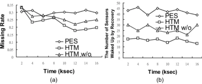
(b) (a) 0 0.05 0.1 0.15 0.2 0.25 0.3 0.35 2 4 6 8 10 12 14 16 Time (ksec) Mi s s ing R a te PES HTM HTM w/o 0 5 10 15 20 25 30 35 40 45 50 2 4 6 8 10 12 14 16 Time (ksec) Th e Numb er o f S ens or s Wak ed U p by Reco ver y PES HTM HTM w/o
Figure 4. (a) The average missing rates be-tween PES, HTM and HTM w/o (b) The average number of nodes participated in the recovery procedure.
will be performed by waking up sensor nodes. The missing rate of two scheme is shown in Figure 4(a).
The number of sensor nodes waken up under PES and HTM is shown in Figure 4(b). By utilizing object moving patterns, HTM is able to accurately predict the movements of objects and then the number of executing the recovery procedure is small. Note that the impact of storage bal-ance to moving patterns is shown. In HTM w/o, cluster heads that store too many levels of information will reduce the accuracy of prediction. Furthermore, due to the very hierarchical nature of HTM, once the recovery procedure is performed, only a bound number of sensors activate for tracking objects. Thus we can conclude that load-balance storage scheme improves the accuracy of prediction.
4.3 Sensitivity Analysis of Storage Replacement Strategy
To conduct the experiments of various β for emission tree node maturity verification, the value of α is set to 0.01. Figure 5 shows the predication rates with the value of β var-ied. As can be seen in Figure 5, the value of β should not set too small or too large. If the emission tree training just gets starting, it is possible that the probability difference is very small when the cluster head receives the same record for a few times. Thus, with a smaller value of β, tree nodes do not collect sufficient moving information for prediction. Once the value of β is too large, tree nodes are hard to be-come mature nodes. Even though tree nodes collect enough moving information, these tree nodes are not able to use for prediction. Clearly, the selection of β will be dependent upon the moving behavior of objects and can be determined empirically. 0.72 0.74 0.76 0.78 0.8 0.82 0.84 5 10 ß 15 20 P red icti o n H it R at e MinSup=25 MinSup=50 MinSup=75
Figure 5. The impact of β for emission tree node maturity verification.
5 Conclusions
In this paper, we proposed a heterogeneous tracking model, called HTM, to efficiently mine object moving terns and track objects. Since HTM relies on moving pat-terns to predict, storage management is an important issue. In this paper, we proposed a load-balance storage scheme for HTM that satisfies storage load-balanced and thus en-sure the quality of moving patterns in each cluster head. Furthermore, when a storage of a cluster head is full, we also developed a storage replacement strategy. Simulation results show that HTM with our proposed storage manage-ment can achieve the best performance to improve the ac-curacy and thus saves energy for tracking objects.
References
[1] M.-S. Chen, J. Han, and P. S.Yu. Data Mining: An Overview from Database Perspective. IEEE
Transac-tions on Knowledge and Data Engineering, 8(6):866–
883, December 1996.
[2] M. Y. et al. Exploiting heterogeneity in sensor net-works. In Proceedings of 24th Annual Joint Conference
of the IEEE Computer and Communications Societies (INFOCOM 2005), 2005.
[3] C.-Y. Lin and Y.-C. Tseng. Structures for in-network moving object tracking in wireless sensor networks. In
BROADNETS, pages 718–727. IEEE Computer
Soci-ety, 2004.
[4] W.-C. Peng and M.-S. Chen. Developing Data Alloca-tion Schemes by Incremental Mining of User Moving Patterns in a Mobile Computing System. 15(6), 2003. [5] Y. Xu, J. Winter, and W. C. Lee. Prediction-based
Strategies for Energy Saving in Object Tracking Sen-sor Networks. In Proceedings of the 2004 IEEE
International Conference on Mobile Data Manage-ment(MDM’04), 2004.
[6] J. Yang and W. Wang. Agile: A general approach to detect transitions in evolving data streams. In
Proceed-ings of ICDM, pages 559–562. IEEE Computer Society,