Updating Generalized Association Rules with
Evolving Fuzzy Taxonomies
Wen-Yang Lin1, Ja-Hwung Su2, and Ming-Cheng Tseng3 1
Dept. of Computer Science and Information Engineering, National University of Kaohsiung, Kaohsiung City, Taiwan;2Dept. of Information Management, Kainan University, Taoyuan, Taiwan;3Refining Business Division, CPC Corporation, Taiwan
Tel: +886-7-5919517 Fax: +886-7-5919514
Email:[email protected];[email protected];[email protected]
Abstract. Mining generalized association rules with fuzzy taxonomic structures has been
recognized as an important extension of generalized associations mining problem. To date most work on this problem, however, required the taxonomies to be static, ignoring the fact that the taxonomies of items cannot necessarily be kept unchanged. For instance, some items may be reclassified from one hierarchy tree to another for more suitable classification, abandoned from the taxonomies if they will no longer be produced, or added into the taxonomies as new items.
Additionally, the membership degrees expressing the fuzzy classification may also need to be adjusted. Under these circumstances, effectively updating the discovered generalized association rules is a crucial task. In this paper, we examine this problem and propose two novel algorithms, called FDiff_ET and FDiff_ET*, to update the discovered generalized frequent itemsets. Empirical evaluations show that our algorithms can maintain their performance even in high degree of taxonomy evolution, and are significantly faster than applying the contemporary fuzzy generalized association mining algorithm FGAR to the database with evolving taxonomy.
Keywords. Data mining; Fuzzy taxonomy; Frequent itemsets; Generalized association rule; Rule maintenance
1. Introduction
Mining generalized association rules is to discover the co-occurred relationships between items as well as their generalization in a taxonomy structure from a transaction database. Consider the taxonomy in Fig. 1. It is very likely we can discover an association rulePC Printer that reveals most of customers who buy PC also tend to buy printer, even though the association between more specific products of them, for example, Notebook and Laser Printer, does not hold.
Since Srikant and Agrawal (1995) introduced the problem of mining generalized association rules from transaction database with taxonomy information, lots of subsequent researches on algorithmic improvement or model extension have been conducted. One of the prosperous avenues on extending generalized association mining is to consider fuzzy taxonomy (Wei and Chen 1999), in which the child-node can partially belong to its parent-child-node with a certain degree in (0, 1). For example, consider the fuzzy taxonomy in Fig. 1, wherein HP Officejet is regarded as being both Printer and Scanner, but to different membership degrees.
Laser HP Officejet ScanMaker Printer Scanner Peripheral PC Desktop Notebook 1 1 1 1 1 1 0.7 0.3
Fig. 1. An example of fuzzy taxonomy T.
To our best knowledge, all work to date on generalized association rules with fuzzy taxonomies assumes that the taxonomic structure is static, not considering the situation that the taxonomy may change as time passes; some items will be shifted from one classification to another, some trees of the taxonomies will be merged together or be split into smaller trees if the items on the trees cannot meet the demands in a new classification, items will be abandoned if those items do not be produced any more, and newborn items are added. Additionally, the
membership degrees expressing the fuzzy classification may also need to be adjusted. Under these circumstances, how to update the discovered generalized association rules effectively becomes a critical task. Our previous work (Tseng et al. 2008; Tseng et al. 2008) has studied this problem of updating generalized association rules but the taxonomy structure is crisp. In this paper, we extend our work to deal with the issue that the taxonomy is fuzzy. Two algorithms, FDiff_ET and FDiff_ET*, are proposed to accomplish the task of updating generalized association rules when the fuzzy taxonomy is evolved. Empirical evaluations show that our algorithms can maintain their performance even in high degree of taxonomy evolution, and are significantly faster than applying the contemporary fuzzy generalized association mining algorithm FGAR (Chen and Wei 2002) to the database with evolving taxonomy.
The remainder of the paper is organized as follows. A review of related work is given in Section 2. The problem of updating previously discovered generalized association rules when the fuzzy taxonomic structure evolves is formalized in Section 3. In Section 4, we elaborate on the proposed two algorithms and give an example to illustrate the ideas. Empirical evaluation of the proposed algorithms with the FGAR algorithm using synthetic dataset is described in Section 5. Finally, our conclusions are stated in Section 6.
2. Related Work
The problem of mining association rules in presence of taxonomy information was first addressed by Han and Fu (1995) and Srinkant and Agrawal (1995), independently. Srinkant and Agrawal (1995) named the problem as mining generalized association rules, aiming to find associations among items at any crossing levels of the taxonomies under the minimum support and minimum confidence constraints. The problem concerned by Han and Fu (1995) was somewhat different in that they generalized the uniform minimum support constraint to a level-wise assignment, i.e., items at the same level received the same minimum support. The objective is to develop mining associations level-by-level in a fixed hierarchy. That is, only associations among items on the same level are examined progressively from the top level to the bottom. Since then, several algorithmic improvements (Huang and Wu 2002; Sriphaew and
Theeramunkong 2004) or problem extensions (Domingues and Rezende 2005; Tseng and Lin 2007) have been proposed.
The problem of mining generalized association rules with fuzzy taxonomic structures was first proposed by Wei and Chen (1999). Later they proposed an extension of the Apriori algorithm, namely FGAR, to accomplish this mining task (Chen and Wei 2002). Various extensions of their work have been made recently, including the concept of introducing generalized weights to distinguish the importance of items in the taxonomy (Kaya and Alhajj 2006; Shen et al. 2005), quantitative attributes (Hong et al. 2003; Wang et al. 2005), multiple minimum supports (Lee et al. 2008), and attribute generalization (Angryk and Petry 2005; Petry and Zhao 2009).
Compared with the substantial amount of research work on mining generalized association rules, there is a lack of effort devoted to the problem of mining
generalized associations with taxonomy evolution. We have considered this problem (Tseng et al. 2008) and some of its extensions, and have proposed efficient Apriori-like algorithms.
3. Problem Statement
3.1 Mining Generalized Association Rules with Fuzzy Taxonomies
Let I{i1, i2, …, im} be a set of items and DB = {t1, t2,…,tn} be a set of
transactions, where each transaction tiTID, Shas a unique identifier TID and a set of items S (SI). We assume that the fuzzy taxonomy of items, T, is available and is denoted as a directed acyclic graph on IJ, where J = {j1, j2, …, jp}
represents the set of generalized items derived from I. An edge in T denotes an
is-a relis-ationship, this-at is, if there is is-an edge from j to i, we cis-all j is-a pis-arent
(generalization) of i and i a child of j. For example, in Fig. 1 I = {Laser, HP Officejet, ScanMaker, Desktop, Notebook} and J = {Scanner, Printer, PC, Peripheral}.
In a crisp taxonomy, we assume that the child item belonging to its ancestor has a membership degree with 1. But in a fuzzy taxonomy, the membership degree of an item may relate to all nodes of the taxonomy. For any two nodes x and y in the taxonomy, the membership degreexyof an item y belonging to its ancestor node
x can be calculated as follows (Wei and Chen 1999): xy=
y x l
: (e onlle) (1)
where l: xy is one of the paths of accessing x from y, e on l is one of the edges on path l, andleis the membership degree on the edge e on l. Operatorsand depend on the problem of concern. For illustrative purposes, max stands forand min for. Furthermore,xxis set to 1, indicating that any item is fully belonging to itself.
Next, consider calculating the support of items under a fuzzy taxonomy. If a is an item in a certain transaction tDB, and x is an item in certain itemset X, then the membership degreexawith which a belongs to x can be obtained according to (1). Finally, the support sup(X) = count(X)/|DB|, where count(X) denotes the
accumulated degree that every transaction supports X in DB, calculated as follows: ) max ( min ) ( xa DB t x X a t DB t tX X count
Example 1 Consider Fig. 1. The membership degreePeripheralLasermin
{(Printer, Laser),(Peripheral, Printer)}min {1, 1} 1. Similarly,PeripheralOfficejet
max {min {(Printer, officejet),(Peripheral, Printer)}, min {(Scanner, officejet),(Peripheral, Scanner)}max {min {0.7, 1}, min {0.3, 1}} = 0.7. Now consider the transaction
database in Table 1. Let X = {Peripheral, PC}. The degree that the first
transaction supports X is min {max {PeripheralLaser,PeripheralHP Officejet}, max
{PCLaser,PCHP Officejet} = min {max {1, 0.7}, max {0, 0}} = 0.
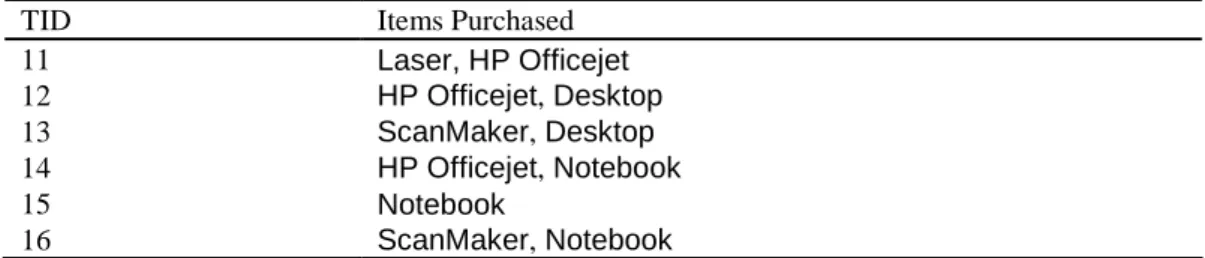
Table 1. An example transaction database (DB).
TID Items Purchased
11 Laser, HP Officejet 12 HP Officejet, Desktop 13 ScanMaker, Desktop 14 HP Officejet, Notebook 15 Notebook 16 ScanMaker, Notebook
Given a set of transactions DB and a fuzzy taxonomy T, a generalized association rule is an implication of the following form
A B,
where A, BI J, A B , and no item in B is an ancestor of any item in A. The support of this rule, sup(A B), is equal to the support of A B. The confidence of the rule, conf(A B)sup(AB)sup(A), is the fraction of
transactions in DB containing A that also contain B. For example, the following is a generalized association rule generated from the transactions in Table 1 with the taxonomy in Fig. 1, with support of 22% and confidence of 65%.
Notebook Scanner (supp 22%, conf 65%)
Definition 1 The problem of mining generalized association rules from a set of transactions DB with a fuzzy taxonomy T is to find all generalized association rules that have support and confidence no less than a user-specified minimum support (ms) and minimum confidence (mc), respectively.
The task of mining generalized association rules is usually decomposed into two steps:
1. Frequent itemset generation: generate all itemsets that exceed the ms. 2. Rule construction: construct all association rules that satisfy mc from the
frequent itemsets in Step 1.
It has been shown in the literature that the process for generating frequent itemsets requires lots of computations as well as I/O operations whereas the rule
construction is straightforward and quite simple compared with the frequent itemset generation. For this reason, the problem of mining generalized association rules is usually reduced to the problem of finding all frequent itemsets for a given minimum support ms.
After an initial discovery of all the generalized association rules in DB, let L be the set of all generalized frequent itemsets with respect to ms. As time passes, some update activities may occur to the taxonomies due to various reasons (Han and Fu 1994). Let T’denote the updated taxonomies. The problem of updating discovered generalized association rules in DB is to find the set of frequent itemsets L’with respect to the refined taxonomies T’.
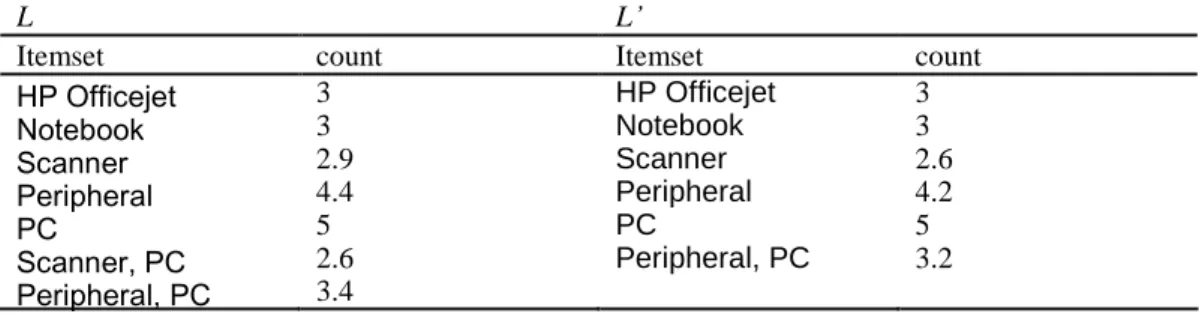
Example 2 Suppose that the taxonomy in Fig. 1 is refined to that in Fig. 2, with the inclusion of a new subcategory of peripheral, Fax, as well as the adjusting of membership degrees of HP Officejet. Let ms42%, i.e., minimum count 2.5. The sets of frequent itemsets with respect to the old taxonomy L and the new taxonomy L’are shown in Table 2.
Fig. 2. A refined fuzzy taxonomy of T in Fig. 1.
Table 2. The sets of frequent itemsets L and L’w.r.t. the taxonomies in Fig. 1 and Fig. 2,
respectively.
L L’
Itemset count Itemset count
HP Officejet 3 HP Officejet 3 Notebook 3 Notebook 3 Scanner 2.9 Scanner 2.6 Peripheral 4.4 Peripheral 4.2 PC 5 PC 5 Scanner, PC 2.6 Peripheral, PC 3.2 Peripheral, PC 3.4
Laser HP Officejet ScanMaker Printer Scanner Peripheral PC Desktop Notebook 1 1 1 1 1 1 Fax 1 0.2 0.2 0.6
3.2 Types of Taxonomy Updates
Our previous work (Tseng et al. 2008) has identified four basic types of item updates that will cause taxonomy evolution, item insertion, item deletion, item
rename, and item reclassification. The essence of frequent itemsets update for
each type of taxonomy evolutions is further clarified in what follows. A new type of taxonomy update specific to the fuzzy taxonomic structure is introduced as well. Note that hereafter the term “item”refers to a primitive or a generalized item.
Type 1: Item insertion. The strategies to handle this type of update operation are different, depending on whether the inserted item is primitive or generalized. When the new inserted item is primitive, we cannot process this item until there is an incremental database update, because the new item does not appear in the original set of frequent itemsets. On the other hand, if the new item represents a generalization, then the insertion itself also has no effect on the discovered associations until the new generalization incurs some item reclassification. Fig. 3 shows an example of this type of taxonomy evolution, where a new item “J”is inserted as a primitive item or a generalized item. Note that in Fig. 3b item “E”is reclassified to the generalization represented by “J”.
A G C I D B F H E J A G C I D B F H J E (a) (b)
Fig. 3. An example of taxonomy evolution caused by item insertion. The inserted item “J” is:(a)
primitive; (b) generalized.
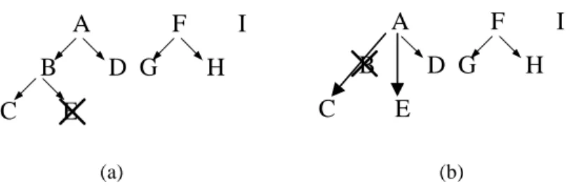
Type 2: Item deletion. This case is similar to the insertion case. Nothing has to be done with the deletion of a primitive item if there is no transaction update to the original database. Notably the removal of a generalization may lead to items reclassification. Fig. 4 shows an example of this type of taxonomy evolution.
Type 3: Item rename. When items are renamed, we do not have to process the database. Instead, we just replace the frequent itemsets with new names and so the association rules. A G C I D B F H A G C I D B F H E E (a) (b)
Fig. 4. An example of taxonomy evolution caused by item deletion:(a)Theprimitiveitem “E”is
deleted; (b) The generalized item “B”isdeleted,and items“C”and “E”arereclassified to “A”.
Type 4: Item reclassification. Among the four types of taxonomy updates this is the most profound operation. Once an item, primitive or generalized, is
reclassified into another category, all of its ancestor (generalized items) in the old and the new taxonomies are affected. In other words, the supports of these
affected generalized items have to be updated and so do the frequent itemsets containing any one of the affected generalized items. For example, in Fig. 5, the two shifted items E and G will change the support counts of generalized items A, B, and F, and also affect the support counts of itemsets containing A, B, or F. Intuitively, these four basic types of operations work on a fuzzy taxonomic structure as well. But an additional operation has to be included to accomplish the situation of membership adjustment.
A G C I D B F H E A E C I G B F H D
Fig. 5. An example of taxonomy evolution caused by item reclassification.
Type 5: Membership adjustment. This operation refers to adjusting the
membership degree of an item in the taxonomy. For example, one may change in Fig. 1 the degrees that HP Officjet belongs to Printer and Scanner to 0.8 and 0.2, respectively. Unlike item reclassification, adjusting the membership of an item x does not change the characteristic (primitive or generalized) of x.
Therefore, it has no effect on the support counting of x if x is primitive; instead it would change the support counting of the ancestors of x.
In this paper, we assume that there is no transaction update to the original database. That is, the transaction database is unchanged before and after the evolution of taxonomic structure.
4. The Proposed Methods
Let ED denote the extended version of DB by adding in taxonomies T the ancestors of each primitive item to each transaction, while ED’denotes the extension of DB by adding generalized items in the updated taxonomies T’. A straightforward method to find updated generalized frequent itemsets would be to run the FGAR algorithm proposed by Chen and Wei (2002) for finding
generalized frequent itemsets on the updated extended transactions ED’. This simple way, however, ignores the fact that many discovered frequent itemsets would not be affected by the taxonomy evolution. If we can identify the unaffected itemsets, then we can avoid unnecessary computations in counting their supports. In view of this, we adapt the Apriori-like maintenance framework we used previously (Tseng et al. 2008). Each pass of mining the frequent k-itemsets involves the following main steps:
1. Generate candidate k-itemsets Ckfrom the discovered set of frequent (k-1)-itemsets L’k.
2. Differentiate in Ckthe affected itemsets (Ck) from the unaffected ones (
k C ). 3. Incorporate Lk, Ck, and k
C to determine whether a candidate itemset is frequent or not in the resulting database ED’.
4. Scan DB with T’, i.e., ED’, to count the support of itemsets that are undetermined in Step 3.
The first step can be accomplished following the apriori-gen procedure used in the well-known Apriori algorithm (Agrawal and Srikant 1994), that is, a candidate k-itemset is formed by joining two different frequent (k-1)-k-itemsets with the same prefix. The last step is conceptually trivial but needs careful implementation for efficiency concern. In the literature, there are two main approaches for
accomplishing this step. One is to adopt the hash-tree structure to store the candidate itemsets, and perform subset operation to efficiently match the
candidate and update the count (Agrawal and Srikant 1994). Another one is keeping the transaction ids, called tid-list, for each item, and performing vector intersection to count the support of each itemset (Zaki 2000). For details, please refer to the book by Tan et al. (2006). In this study, we adopt the second approach because it is more efficient than the first one. Below, we elaborate on each of the kernel steps, i.e., Steps 2 and 3.
4.1 Differentiation of Affected and Unaffected Itemsets
Definition 2 An item (primitive or extended) is called an affected item if its support would be changed with respect to the taxonomy evolution; otherwise, it is called an unaffected item.
Consider an item xT T’and the three independent subsets T T’, T’T and T T’. There are three different cases in differentiating whether x is an affected item or not. The case that x is a renamed item is neglected for which can be simply regarded as an unaffected item.
Case 1. xT T’. That is, x is an obsolete item. Then the support of x in the updated database should be counted as 0 and so x is an affected item.
Case 2. xT’T. That is, x denotes a new item. If x is a primitive item, it does not appear in the database and so can be regarded as an unaffected item.
Otherwise, x should be regarded as an affected item since its count would change from zero to nonzero.
Case 3. xT T’. This case depends on whether x is a primitive item both in T and T’or not. Obviously, if x is primitive, there is no change on its support and so
x is an unaffected item; otherwise, the count of x may change or not, depending on
whether any of its descendants is involved in any evolution operation of item reclassification or membership adjustment. Recall that in (2) the support counting of an itemset is primarily determined by calculating the membership degree in (1). Thus we can derive a simple rule for determining x as affected or not, as clarified in the following lemma.
Lemma 1 Consider an item xT T’. Let Q(x) and Q’(x) denote in T and T’, respectively, the set of primitive descendants of x, each along with their
membership degrees with respect to x. More specifically, Q(x){(y1,xy1), (y2,
xy2), …, (yn,xyn)} and Q’(x){(y’1,xy’1), (y’2,xy’2), …, (y’m,xy’m)}, where {y1, y2,…, yn} and {y’1, y’2, …, y’m} are the descendants of x in T and T’, respectively.
If Q(x)Q’(x), then countED(x)countED’(x), where Q(x)Q’(x) means mn; y1
y’1, …, yny’n; andxy1xy’1, …,xynxy’n.
Proof: Consider a transaction t in DB. If t supports x with respect to ED, there
exists at least one item being primitive descendant of x in T, say d1, d2, …, diand
{d1, d2, …, di}{y1, y2,…, yn}. Likewise, if t supports x with respect to ED’, then
there must exist at least one item being primitive descendant of x in T’, say {d’1, d’2, …, d’j} and {d’1, d’2, …, d’j}{y’1, y’2,…, y’m}. Since mn and y1 y’1, …, yny’n, it follows that ij and d1d’1, …, did’i. Further,xd1
xd’1, …,xdixd’i. According to (2), the degree that t supports x in ED is equal to
that in ED’. The lemma then follows.
Example 3 Continue with Example 2. Clearly, Fax is an affected item (Case 2). Now consider the generalized items satisfy Case 3, i.e., Printer, Scanner,
Peripheral, and PC. PC is unaffected since it possesses the same set of primitive descendants, each of which retains the same membership degree. However, Printer, Scanner, and Peripheral are affected items. Although each of them has the same set of primitive descendants, at least one of its primitive descendants changes the membership degree.
Definition 3 For a candidate itemset A, we say A is an affected itemset if it contains at least one affected item.
4.2 Inference of Frequent and Infrequent Itemsets
Now that we have clarified how to differentiate the unaffected and affected itemsets, we will show how to utilize this information to determine in advance whether or not an itemset is frequent before scanning the updated extended database ED’. We observe that there are four different cases.
1. If A is an unaffected itemset and is frequent in ED, then it is also frequent in
ED’.
2. If A is an unaffected itemset and is infrequent in ED, then it is also infrequent in ED’.
3. If A is an affected itemset and is frequent in ED, then it may be frequent or infrequent in ED’.
4. If A is an affected itemset and is infrequent in ED, then it may be frequent or infrequent in ED’.
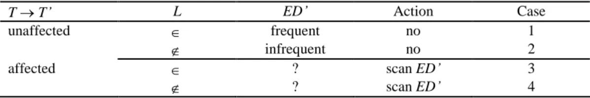
Note that only cases 3 and 4 need further database scan to determine the support count of A. Table 3 summarizes the above discussion.
Table 3. The cases of inferring whether a candidate itemset is frequent or not.
T T’ L ED’ Action Case
unaffected frequent no 1
infrequent no 2
affected ? scan ED’ 3
? scan ED’ 4
4.3 Algorithm FDiff_ET
Based on the aforementioned concepts, the proposed FDiff_ET algorithm is described in Fig. 6.
Input: (1) DB: the original database; (2) ms: the minimum support; (3) T: the old fuzzy taxonomy; (4) T’: the new fuzzy taxonomy; (5) L: the set of old frequent itemsets.
Output: L’: the set of new frequent itemsets. Steps:
1. C1be set of all items in T’excluding new primitive items;
2. Create MD and MD’; /* the table of membership degree using (1) */ 3. C1
+
= iden_AFItem(C1, MD, MD’, T, T’); /*Identify all affected items. */
4. k1; 5. repeat
6. if k > 1 then
7. Ckapriori-gen(L’k1);
8. delete any candidate in Ckthat consists of an item and its ancestor; 9. endif
10. load original set of frequent k-itemsets Lk; 11. divide Ckinto two subsets:
k
C andCk; 12. for each A
k
C do
13. if ALkthen supED’(A)supED(A); /* Cases 1*/ 14. else delete A from
k
C ; /* Case 2 */ 15. scan ED’to count count
ED’(A) according to (2) for each itemset A in
k C ; /* Cases 3 & 4 */ 16. L’ k k
C {A | ACkand supED’(A)ms}; k++; 17. until L’k1
18. L’kL’k;
Fig. 6. Algorithm FDiff_ET.
First, let candidate 1-itemsets C1be the set of items in the new item taxonomies T’. Next derive the membership degree among all items in C1represented as a
matrix and identify affected items for dividing candidate itemsets. Then load the original frequent 1-itemsets L1and divide C1into two subsets: C1 and
1
consists of unaffected 1-itemsets in L1, and C1 contains affected 1-itemsets,
where C is for cases 1 and 2, and1 C is for cases 3 and 4. According to case 2,1
all itemsets inC that is not in L is infrequent and so are pruned. Then compute1
the support counts of each 1-itemset in C1over ED’. After this, we create new frequent 1-itemsets Lby combining1 C and those itemsets being frequent in1
1
C . The next cycle is that we generate candidates 2-itemsets C2from Land1
repeat the same procedure until no frequent k-itemsetsLkare created.
4.4 Algorithm FDiff_ET*
The second algorithm FDiff_ET* is an improvement of FDiff_ET. We observe that for cases 3 and 4 in Table 3 there is no need to scan the whole ED’to count the supports of affected itemsets. Instead, it suffices to scan those transactions that are affected with respect to the taxonomy evolution.
Definition 4 A transaction is called an affected transaction if it contains at least one of the affected items with respect to a taxonomy evolution.
The intuition behind Definition 4 is that an affected transaction would contribute to the support change of affected itemsets. Note that this definition is a general description; it can refer to any kind of transaction database concerned in this study, i.e., DB, ED, or ED’. To be more precise, we useto denote the set of affected transactions with respect to the taxonomy evolution T T’, and introduce subscript DB, ED, or ED’for database distinction.
Lemma 2 Consider an affected itemset X with respect to T T’. We have
countDB(X)countDB(X), countED(X)countED(X), countED’(X)countED’(X). Proof: We only prove the case for ED’since it is similar for the other two cases.
According to Definition 4, X only appears inED’. That is, countED’ED’(X) = 0.
The lemma then follows.
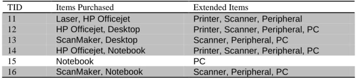
Example 4 Consider the transaction database in Table 1 again. Since the affected items with respect to taxonomy evolution from Fig. 1 to Fig. 2, i.e., Fax, Printer, Scanner, Peripheral, all are generalized items, there is no affected transaction in Table 1 according to Definition 4. The corresponding extended transaction
database ED by inserting generalized items in taxonomies T and the updated extended transaction ED’by inserting generalized items in taxonomies T’are shown in Table 4 and Table 5, respectively, where those shaded transactions
denote the affected part. It is easy to verify the phenomenon stated in Lemma 2. For example, consider itemset {HP Officejet, Fax}. It is an affected itemset since it contains an affected itemFax. Obviously, {HP Officejet, Fax} can appear only in the part of affected transactions, either in ED or ED’, i.e., countED({HP
Officejet, Fax}) countED({HP Officejet, Fax}) 0, and countED’({HP
Officejet, Fax}) countED’({HP Officejet, Fax}) 3. Note that although both
sets of affected transactions in Tables 4 and 5 are derived from the same set of original transactions in Table 1, the contents are different.
Table 4. The extended transaction database ED.
TID Items Purchased Extended Items
11 Laser, HP Officejet Printer, Scanner, Peripheral 12 HP Officejet, Desktop Printer, Scanner, Peripheral, PC 13 ScanMaker, Desktop Scanner, Peripheral, PC
14 HP Officejet, Notebook Printer, Scanner, Peripheral, PC
15 Notebook PC
16 ScanMaker, Notebook Scanner, Peripheral, PC
Table 5. The updated extended transaction database ED’.
TID Items Purchased Extended Items
11 Laser, HP Officejet Printer, Scanner, Fax, Peripheral 12 HP Officejet, Desktop Printer, Scanner, Fax, Peripheral, PC 13 ScanMaker, Desktop Scanner, Peripheral, PC
14 HP Officejet, Notebook Printer, Scanner, Fax, Peripheral, PC
15 Notebook PC
16 ScanMaker, Notebook Scanner, Peripheral, PC
According to Definition 4, identification of affected transactions requires a database scan, which fortunately is avoidable if we embed the identification within the support counting of 1-itemsets. This means no cost saving can be obtained by confining the counting of affected 1-itemsets over affected
transactions. This pay-off is worthy because the counting of 1-itemsets involves no combinatorial subset enumeration. Revising Step 15 in Fig. 6 as shown in Fig. 7 accomplishes the description of algorithm FDiff_ET*.
15'. if k = 1 then
scan ED’to identify affected transactionsED’and count countED’(A) according to (2) for each itemset A in Ck;
else
scanED’to count countED’(A) according to (2) for each itemset A in Ck; endif
5. Experimental Results
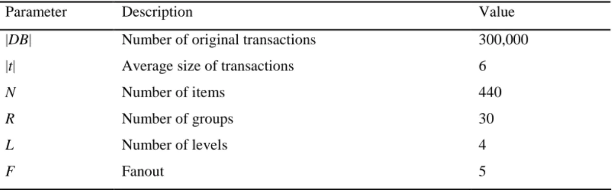
In order to examine the performance of FDiff_ET and FDiff_ET*, we conducted experiments to compare them with FGAR, using the synthetic dataset generated by the IBM data generator (Agrawal and Srikant 1994) with an artificially-built fuzzy taxonomy composed of 440 items that are divided into 30 groups, each of which consists of four levels with average fanout of 5. The default parameter settings are shown in Table 6.
Table 6. Default parameter settings for test datasets.
Parameter Description Value
|DB| Number of original transactions 300,000
|t| Average size of transactions 6
N Number of items 440
R Number of groups 30
L Number of levels 4
F Fanout 5
The comparisons were evaluated from various aspects, including the differences in minimum supports, data sizes, transaction lengths, and evolution degrees. Here, the evolution degree is measured by the fraction of affected items. Since FGAR possesses no updating mechanism to deal with the taxonomy evolution, it was executed from scratch each time when the taxonomy changes. All programs were coded in C and all experiments were performed on an Intel Celeron Dual-Core E3300 2.50Hz CPU with 2MB RAM, running on Windows XP.
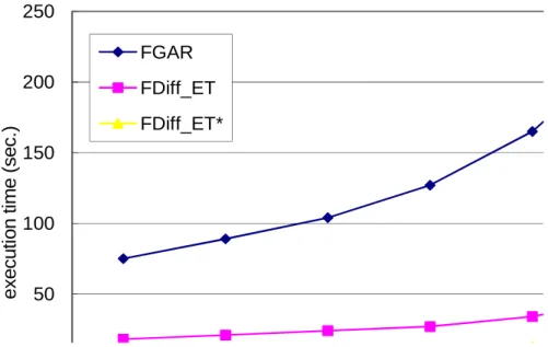
Minimum supports: We first compared the performance of the three algorithms with varying minimum supports at constant evolution degree 10%; the number of transactions, fanout and groups were set to default values. As the results shown in Fig. 8, the execution times of all three algorithms grow exponentially with respect to a linear decrease of minimum support, owing to the combinatorial explosion of candidate itemsets. The results also reveal that the performance of FGAR is much more affected by the minimum support compared with our proposed algorithms. This is because FGAR embraces no updating mechanism. Our algorithms, on the contrary, alleviate the effect of combinatorial explosion by identifying the set of affected itemsets, and so can significantly save the cost for recomputing the supports of unaffected itemsets. FDiff_ET* outperforms FDiff_ET because
FDiff_ET* confines support counting of affected itemsets to be executed over the affected transactions.
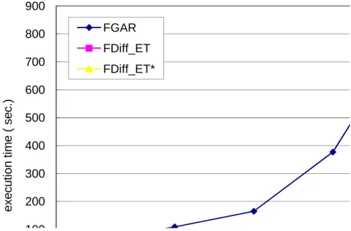
Data sizes: We then compared the three algorithms under varying data sizes at ms 1.0% with constant affected item percent 10%. The other parameters were set to default values. The results are depicted in Fig. 9. All algorithms exhibit linear scalability, though FGAR displays the worst scalability and FDiff_ET* performs the best.
Transaction length: Next, we inspect the performance impact of varying transaction length. In this experiment, the minimum support was set at 1%, evolutionary degree to 10%, and other parameters were set to default values. The results as depicted in Fig. 10 are quite similar to those in Fig. 8. This is because increasing the transaction length has analogous effect on combinatorial explosion of subset enumeration and inspection. FDiff_ET*, however, does not significantly outperform FDiff_ET as observed in Fig. 8. The reason is that the performance gain of FDiff_ET* over FDiff_ET is contributed by the cost saving on support counting of affected itemsets; only the affected transactions have to be scanned and the amount of which is mainly dependent on the degree of taxonomy evolution10% in this case.
Evolution degree: Finally, we compared the algorithms under varying degrees of evolution with ms1.0%. The other parameters were set to default values. In this experiment, the affected items were generated by performing random item
reclassification or membership adjustment. Intuitively, with more affected items, there should be more affected itemsets as well as more affected transactions. This explains the results shown in Fig. 11: Our algorithms are greatly affected by the degree of evolution with performance decreasing with respect to the increasing of evolution degree, whereas FGAR exhibits steady performance. FDiff_ET*
overwhelms FDiff_ET in all cases, the performance gain rising proportionally to the evolution degree. This is because the increase in the amount of affected candidate itemsets is far more than that of affected transactions, thus aggravates the benefit obtained from confining support counting over affected transactions. In summary, our proposed algorithms are significantly faster than FGAR and exhibit good scalability. FDiff_ET* outperforms FDiff_ET in all cases, especially less prone to the effect of high degree of taxonomy evolution.
50 100 150 200 250 e x e c u ti o n ti m e (s e c .) FGAR FDiff_ET FDiff_ET*
Fig. 8. Performance comparison of FGAR, FDiff_ET, and FDiff_ET* with varying minimum
supports. 20 40 60 80 100 120 140 160 180 e x e c u ti o n ti m e (s e c .) FGAR FDiff_ET FDiff_ET*
100 200 300 400 500 600 700 800 900 e x e c u ti o n ti m e ( s e c .) FGAR FDiff_ET FDiff_ET*
Fig. 10. Performance comparison of FGAR, FDiff_ET, and FDiff_ET* with varying transaction
length. 20 40 60 80 100 120 140 160 180 e x e c u ti o n ti m e (s e c .) FGAR FDiff_ET FDiff_ET*
Fig. 11. Performance comparison of FGAR, FDiff_ET, and FDiff_ET* with varying evolution
degrees.
6. Conclusions
In this paper we have investigated the problem of updating generalized association rules with evolving fuzzy taxonomies. We have elaborated on the
design of two efficient algorithms, FDiff_ET and FDiff_ET*, for updating previously discovered generalized frequent itemsets. Empirical evaluations have shown that our algorithms exhibit good scalability, can maintain their
performance even in high degree of taxonomy evolution, and are significantly faster than applying the FGAR algorithm to the database with evolving taxonomy. Although our work in this study has advanced the research in generalized
associations mining, there are many unexplored issues deserved further
investigation. For example, the study can be extended to a more general model that incorporates multiple minimum supports, weights of items, quantitative database, and even more complicated fuzzy ontological structure (Lee et al. 2010) such as that exploiting both classification and component relationships, and the representation of the fuzzy ontology, e.g., Fuzzy Markup Language (Acampora et al. 2010). Another prospective avenue is on embedding the frequent pattern maintenance scheme into an online data mining platform.
References
Acampora G, Gaeta M, Loia V, Vasilakos AV (2010) Interoperable and adaptive fuzzy services for ambient intelligence applications. ACM Transactions on Autonomous and Adaptive Systems 5(2):1-26.
Agrawal R, Srikant R (1994) Fast algorithms for mining association rules. In: Proc. VLDB, pp 487-499.
Angryk RA, Petry FE (2005) Mining multi-level associations with fuzzy hierarchies. In: Proc. 14th IEEE Int. Conf. on Fuzzy Systems, pp 785-790.
Chen G, Wei Q (2002) Fuzzy association rules and the extended mining algorithms. Information Sciences 147(1-4):201-228.
DeGraaf JM, Kosters WA, Witteman JJW (2001) Interesting fuzzy association rules in quantitative databases. LNCS 2168:140-151.
Domingues MA, and Rezende SO (2005) Using taxonomies to facilitate the analysis of the association rules. In: Proc. 2nd Int. Workshop on Knowledge Discovery and Ontologies, pp 59-66.
Han J, Fu Y (1994) Dynamic generation and refinement of concept hierarchies for knowledge discovery in databases. In: Proc. AAAI’94 Workshop on Knowledge Discovery in Databases, pp 157-168.
Han J, Fu Y (1995) Discovery of multiple-level association rules from large databases. In: Proc. 21st Int. Conf. Very Large Data Bases, pp 420-431.
Hong TP, Ling KY, Wang SL (2003) Fuzzy data mining for interesting generalized association rules. Fuzzy Sets and Systems 138:255-269.
Huang YF, Wu CM (2002) Mining generalized association rules using pruning techniques. In: Proc. IEEE Int. Conf. on Data Mining, pp 227-234.
Kaya M, Alhajj R (2006) Effective mining of fuzzy multi-cross-level weighted association rules. In: Proc. 16th Int. Symp. on Foundations of Intelligent Systems, LNCS 4203, pp 399-408.
Lee CS, Wang MH, Acampora G, Hsu CY, Hagras H (2010) Diet assessment based on type-2 fuzzy ontology and fuzzy markup language. International Journal of Intelligent Systems 25(12):1187-1216.
Lee YC, Hong TP, and Wang TC (2008) Multi-level fuzzy mining with multiple minimum supports. Expert Systems with Applications 34:459-468.
Petry FE, Zhao L (2009) Data mining by attribute generalization with fuzzy hierarchies in fuzzy databases. Fuzzy Sets and Systems 165(15):2206-2223.
Shen B, Yao M, Bo Y (2005) Mining weighted generalized fuzzy association rules with fuzzy taxonomies. In: Proc. Int. Conf. Computational Intelligence and Security, LNCS 3801, pp 704-712.
Srikant R, Agrawal R (1995) Mining generalized association rules. In: Proc. 21st Int. Conf. Very Large Data Bases, pp 407-419.
Sriphaew K, Theeramunkong T (2004) Fast algorithms for mining generalized frequent patterns of generalized association rules. IEICE Transaction on Information and Systems 87(3):761-770.
Tan PN, Steinbach M, Kumar V (2006) Introduction to Data Mining. Addison-Wesley.
Tseng MC, Lin WY (2007) Efficient mining of generalized association rules with non-uniform minimum support. Data and Knowledge Engineering 62(1):41-64.
Tseng MC, Lin WY, Jeng R (2008) Updating generalized association rules with evolving taxonomies. Applied Intelligence 29(3):306-320.
Tseng MC, Lin WY, Jeng R (2008) Incremental maintenance of generalized association rules under taxonomy evolution. Journal of Information Science 34(2):174-195.
Wang S, Chung KFL, Shen H (2005) Fuzzy taxonomy, quantitative database and mining generalized association rules. Intelligent Data Analysis 9(2):207-217.
Wei Q, Chen G (1999) Mining generalized association rules with fuzzy taxonomic structures. In: Proc. 18th Int. Conf. North American Fuzzy Information Processing Society, pp 477-481.
Zaki MJ (2000) Scalable algorithms for association mining. IEEE Transactions on Knowledge and Data Engineering 12(3):372-390.