Affinity Set Based Discretization:
A Multi-Objective Approach
/ 99 ■ 101 6 30 105 6 30
□ ( ) ( ) --- □ BIT097101 100 6 30
4
/
95
2
II
ABSTRACT
This research attempted to construct an affinity based discretization model to generate classification rules, and solve the multi-objective problem of accuracy, number of split points, and number of rules, via particle swarm optimization (PSO). Comparing with traditional affinity set and ant colony optimization (ACO), our proposed model can generate fewer split points and fewer classification rules with higher accuracy.
III
CONTENT
1. INTRODUCTION ... 1 2. LITERATURE REVIEW ... 5 2.1 Classification...6 2.2 Affinity Set ...8 2.3 Discretization ...132.4 Multi-Objective Decision Making ...17
2.5 Particle Swarm Optimization, PSO...21
3. PROPOSED DISCRETIZATION MODEL ... 25
3.1 Research Structure ...25
3.2 Problem Definition...27
3.3 Multi-objective Model ...29
4. CASE ANALYSIS ... 36
4.1 Experiment I: IRIS dataset ...38
4.2 Experiment II: Multiple Enrollment Dataset ...46
5. CONCLUSION ... 56
5.1 Results ...56
5.2 Future Works ...56
IV
LIST OF TABLES
Table 2-1 Instance Samples ...10
Table 3-1 Objectives of our model ...28
Table 3-2 Notations ...29
Table 3-3 Standardization ...31
Table 4-1 Details of datasets ...36
Table 4-2 Main characteristics of the data sets used in the experiments ...37
Table 4-3 Attributes and class coding of IRIS dataset ...39
Table 4-4 Custom dividing point for ACO and Traditional Affinity Set ...40
Table 4-5 Parameters settings for experiment I ...41
Table 4-6 Rule set from ant colony optimization ...42
Table 4-7 Rule set from multi-objective affinity set ...43
Table 4-8 Dividing point for multi-objective affinity set ...44
Table 4-9 Classification results of experiment I ...45
Table 4-10 Attributes and class coding of IRIS dataset ...47
Table 4-11 Custom dividing point for ACO and traditional Affinity Set ...48
Table 4-12 Parameters settings for experiment I ...49
Table 4-13 Rule set from ant colony optimization ...50
Table 4-14 Rule set from affinity set ...51
Table 4-15 Rule set from multi-objective affinity set ...53
Table 4-16 dividing point for multi-objective affinity set ...54
V
LIST OF FIGURES
Figure 1-1 Research Process ...4
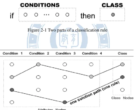
Figure 2-1 Two parts of a classification rule ...6
Figure 2-2 Each path denotes a classification rule...6
Figure 2-3 Discretization Process ...14
Figure 2-4 Pareto Solution ...19
Figure 3-1 Research structure ...26
Figure 3-2 Proposed Multi-objective Model...30
Figure 3-3 randomly select dividing points ...33
Figure 3-4 List all possible rule set and calculate affinity degree ...33
Figure 3-5 Iterate selecting rules randomly ...34
Figure 3-6 select dividing bins via PSO ...34
1
1. INTRODUCTION
Classification is an important task of data mining. The process of classification constructs a model from dataset of known attributes to describe the relationship between the observed outcomes (consequences) and the possible incomes (causes) of an information system. A classification task consists of two main steps (Kianmehr, Alshalalfa, & Alhajj, 2008): finding classification rule set through data objects (in the training set), and building a classifier based on the extracted rules to predict the class or categories which was determined by input attributes. According to this classification model (classification rule set), we can analyze and predict new unclassified datasets.
Affinity set algorithm is a relatively new technique mainly used for data mining classification problems (Chen, Larbani, Shen, & Chen, 2008; Chen, Larbani, Wu, & Chen, 2007). Not only all classification rules are visible but also with more selectiveness to choose. The core idea of affinity set is to extract the rule set from all possible rules via the k-core method, which is used to decide chosen rules with the gate value k. However, there is no standard way to determine the value of k, and some selection will generate a huge number of rules in a rule set. The large number of rules makes it overwhelming to extract rules and difficult to interpret and
2
react to the rule set, especially because many rules are often superfluous and contained in other rules (Berrado & Runger, 2007). Furthermore, affinity set algorithms relies on discrete data and need to discretize continuous attributes, which are ordinal data types with orders among the values and often involved in real-world problem or large real-world datasets (Liu, Hussain, Tan, & Dash, 2002).
Continuous attributes (also called numeric attributes) need to be preprocessed and transferred into discrete attributes for many symbolic inductive classification algorithms (Pfahringer, 1995). The process of discretization thus plays an important role in data mining to partition continuous attribute domains into intervals, and map each one as a discrete value. Discretization is beneficial for various reasons (Pfahringer, 1995):
1. Efficiency: Large amount of numerical attributes slows down induction.
2. Intelligibility: Handling noisy, large numerical attributes is complex considerably. 3. Accuracy: Avoiding noisy training examples sometimes increases accuracy.
This research aimed at proposing a novel affinity set based discretization model with higher accuracy, fewer discretization split points and fewer classification rules. However, creating too few rules and split points would probably reduce information and representative in
3
original data, and thus seems to be considered as a multi-objective problem, in which we need to obtain a compromise or trade-off solution between statistical quality (to generate reasonable sized initial split points) and information quality (without losing information in the source numerical data).
Optimization problems rather commonly have more than one objective in every field or area in real world. Objectives in a multi-objective problem are normally in conflict with respect to each other, thus there is no single solution. For finding a good ―trade-off‖ solution that compromises among the objectives, amount of research recently grow in the area of multi-objective optimization (Deb, 2001). Evolutionary algorithms such as Particle Swarm Optimization (PSO) are extended and frequently applied to solve the multi-objective problem (Coello, 2006; Mostaghim, 2003; Pal, 2007).
In this paper, our proposed affinity based model combined particle swarm optimization to solve the multi-objective problem in discretization process. The remainder of this paper is organized as follows. In chapter 2, we provide some basic concept of classification, affinity set, discretization, multi-objective decision making, and particle swarm optimization. Chapter 3 presents our proposed affinity set based discretization model. In chapter 4 we give two
4
experiments of IRIS dataset and multi enrollment dataset to compare our model with ant colony optimization and traditional affinity set. Finally, we present our conclusion and suggestion in chapter 5. Total research process is summarized as follow in Fig. 1-1.
5
2. LITERATURE REVIEW
In this chapter, we first briefly review the concept of classification. Second, we introduce the main idea of affinity set algorithm and k-core method; furthermore, we point out rule choosing problem we faced of k-core method we attempted to improve. In the next section, we give a review of discretization main concept. Multi-objective decision making will be introduced in section 4. In the last section, we explain particle swarm optimization algorithm for applying in multi-objective problem.
6
2.1 Classification
As well known, a classification rule consists of two parts as Fig. 2-1; a rule can be designed as a solution path through at least one of the condition nodes to exact one class node as shown in Fig.2-2. The same attribute appears only once in a rule path.
Figure 2-1 Two parts of a classification rule
.
Figure 2-2 Each path denotes a classification rule
The process of classification constructs a model from dataset of known attributes to describe the relationship of attributes and class. According to this classification model (classification
7
rule set), we can analyze and predict new unclassified datasets. There are numerous algorithms developed for classification, such as neural network, support vector machine, etc. However, the classifier above generates a ―black-box‖ from which we can’t observe exactly classification rules. Relatively, classification algorithms such as decision tree, ant colony optimization, affinity set, etc. generate visible classification rules. Visible classification rules can be more easily applied on real world problems.
In this research, we choose ant colony optimization and affinity set to be our experiment model. They both generate visible classification rules with relatively higher accuracy (Chih-Hung Wu, Lin, Li, Fang, & Wu, 2008; C.-H. Wu, Lin, Li, Fang, & Wu, 2009), and was applied in several research fields (Ahmad & Srivastava, 2008; Yuh-Wen Chen & Larbani, 2007; Y.-W. Chen et al., 2008; Holden & Freitas, 2004; Jensen & Shen, 2006; Piatrik & Izquierdo, 2006).
8
2.2 Affinity Set
From the ancient and oriental culture (Ho, 1998; Hwang, 1987; Luo, 2000), the original meaning of affinity is a close relationship between people or objects that have similar appearances, qualities, structures, properties or features, etc. Mathematically, affinity can be considered as a relation between elements of a set, the subjects, with an object or medium; this relation is the affinity itself. Here we briefly formalize the rigid definitions about the affinity between a subject e and an affinity set as follows (Y.-W. Chen et al., 2008).
Applying affinity set on classification, we consider all possibility of rules combination. It consists of five steps:
(a1) Define the metric space (X, d) (a2) Determine the referential set V
(a3) Determine the core B of the affinity set Use the affinity as defined
d: V[0,1]
ed(e, B)= 1d(e, B)
(a4) Compute the hit rate (affinity degree) of each rule in V (a5) Decide the k-core (A) with a given k
9
In step (1) and (2), a metric space (X, d) is a set endowed with distance d(x, y) (Mendelson &
B, 1990), and it contains all the guess/rules. A guess/rule base V={ri, i1,m} is a subset of X
where ri is one guess/rule. An affinity set A in V is defined as
A= (d, B, V) Eq. 2-1
where d is the affinity defined as step (4). The hit rate is defined as the frequency of accurate prediction divided by the number of samples. The set B is called the core of the affinity set A. The distance between an element e of V and the subset B of V is defined as
d(e, B)= minzB d(e, z) Eq. 2-2
Notice that d(e, B) is not traditional definition of the distance between two elements. The maximum distance between elements of V is defined as
= xy V V y x ) , ( ) , ( d max 1 Eq. 2-3
10
d(e, B)= minzB d(e, z) = 0
→d(e, B)= 1d(e, B)=10= 1 Eq. 2-4
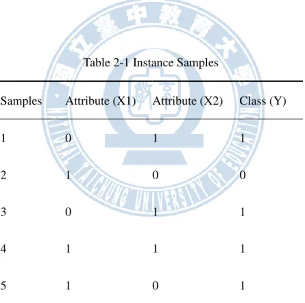
The affinity equals 1 means this element is in the core of the affinity set. Hence Core (A)= B. Now we take an example as follows:
Table 2-1 Instance Samples
Samples Attribute (X1) Attribute (X2) Class (Y)
1 0 1 1
2 1 0 0
3 0 1 1
4 1 1 1
5 1 0 1
There are 8 possible rules:
r1: if X1=1 and X2=1, then y =1, hit rate = 1/5 r2: if X1=1 and X2=1, then y =0, hit rate = 0/5
11
r3: if X1=1 and X2=0, then y =1, hit rate = 1/5 r4 if X1=1 and X2=0, then y =0, hit rate = 1/5 r5: if X1=0 and X2=1, then y =1, hit rate = 2/5 r6: if X1=0 and X2=1, then y =0, hit rate = 0/5 r7: if X1=0 and X2=0, then y =1, hit rate = 0/5 r8: if X1=0 and X2=0, then y =0, hit rate = 0/5
We got the w-0.2-core(A) = {r1, r3, r4, r5} if k =0.2, and the w-0.4-core(A) = {r5} if k =0.4. If a guess/rule has more frequently to hit the observed samples, then such a rule surely has greater affinity (higher accuracy) with A. The simple selection of core of the above is called k-core method. As the sample size increases and as the level of classifying the qualitative attribute increases, we can use such a simple thinking to approximate the affinity set of rule: ―Appropriateness of explaining observed samples‖. In general, the selection of k determines
the quality of a rule set.
However, we face the problem that the total accuracy is not quite depends on the selection of
k (because combining all rules with high affinity degree would not surely increase total
12
difficult to interpret. The number of rules is better smaller for constructing and maintaining a detection support system. Furthermore, to keep the rule set quality in terms of accuracy, fidelity, comprehensibility and consistency (Barakat, 2007) is another obvious goal in classification problems.
Rule extraction task of affinity set can thus be considered for two objectives: fewer rules, higher classification quality. For this reason, our affinity set improvement model will also focuses on these two objectives.
13
2.3 Discretization
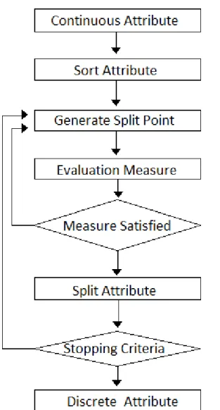
Discretization task is to deal with continuous attributes for machine learning and data mining on the process to partition continuous (real value) attribute domains into intervals, and map each one as a discrete symbolic value (Qu et al., 2008). Discretization can be applied to reduce the amount of data, and simultaneously retain or even improve predictive accuracy (Liu et al., 2002). We clarify discretization process by an abstract description as follow and Figure 2-3.
The first step is to sort values in a feature or attribute in either descending or ascending order. There are already sorting algorithms can be applied, such as quick sort. Notice that a global treatment is to sort at the beginning of discretization without repeatedly sorting; relatively, a local treatment is to sort at each iteration of a process, and consider only a region of entire instance space. A global treatment has higher efficiency, obviously.
14
Figure 2-3 Discretization Process
After sorting, the second step is to generate split points (or called cut points) to split a range of continuous values into intervals. There are simple techniques used to discretize in earlier days, such as equal-width and equal-frequency (or, a form of binning) to discretize; Equal width interval method is perhaps the simplest discretization method to divide the range of sorted observed values into k equally sized bins (Dougherty, Kohavi, & Sahami, 1995;
15
Skubacz & Hollmén, 2008). Equal frequency interval method cuts the attributes into bins with equal number of instance. However, these methods are unsupervised (or called class-blind), and do not use instance class labels while discretization process. Since unsupervised methods do not utilize instance labels, the classification information is likely to be lost without taking information about class into account (Kerber, 1998). Relatively, supervised methods utilize instance labels and the values associated with classes.
Numerous evaluation functions were proposed to find effective split points. Grzymala-Busse gave suggestions as guidelines for a proper discretization method (Grzymala-Busse, 2002): 1. Complete discretization: Majority of current discretization methods is local, which
process only one attribute at one time. In contrast, global methods produce a mesh over the entire instance space simultaneously.
2. Simplest result of discretization: Smaller size of discretized attribute domain leads simpler rule set that saves more storage of classifier and has more generality.
3. Consistency: To prevent data set losing information (called inconsistent) after discretization, one objective is to maintain the consistency. However, consistency conflicts with simplest result of discretization and generality somehow.
16
To prevent data set losing information (called inconsistent) after discretization, one objective is to maintain the consistency. However, consistency conflicts with simplest result of discretization and generality somehow (Grzymala-Busse, 2002). For finding an optimal split point set, the process tends to be a multi-objectives optimization problem.
After generating split points and splitting continuous values into discrete intervals, researchers are able to design an iteration mechanism and stopping criteria for finding an optimal solution. In this paper we aim at constructing a multi-objective model for discretization task.
17
2.4 Multi-Objective Decision Making
Optimization problems in real-world are rather common to have more than one objective, which leads to the need of optimal or effective solutions (Ishibuchi, Nakashima, & Nii, 2005). These objectives sometimes are in conflict with respect to each other (such as improving the quality of a product and reducing the cost), and thus there is no single solution for these problems.
Many proposed methods avoiding the complexities of conflicting goals to convert multi-objective problems into single objective problems, which usually wants to discover a single optimal solution and is a degenerated case of a multi-objective optimization problem, i.e. a multi-objective problem is transformed into a single-objective one. Instead of forcing the user to choose one optimal solution for only one of the conflicting goals, a multi-objective problem usually needs to be solved by several optimal solutions that take all objectives into account, without assigning greater priority to one objective or the other. Therefore, multi-objective decision making techniques seem to be a proper tool for selecting alternatives from a set of options based on the multiple, even conflicting, objectives (Brauers, Zavadskas, Peldschus, & Turskis, 2008).
18
Through multi-objective optimization method, we can find a optimal solution to these objective simultaneously. Basically, there are methods which were rather common applied. 1. Weighting method: Assign a weight for each objective, and combine all weighted
objectives into one objective for finding an optimal solution.
min f(x) = ∑ni=1wi∙ fi(x) Eq. 2-5
or
max f(x) = ∑ni=1wi∙ fi(x) Eq. 2-6
2. Priority method: Based on the priority or user’s choice of each objective, optimization is ordered up-down by major priority.
min f2(x) with 𝑓1(𝑥)ℎ𝑎𝑠 𝑏𝑒𝑒𝑛 𝑜𝑝𝑡𝑖𝑚𝑖𝑧𝑒𝑑 Eq. 2-7 or
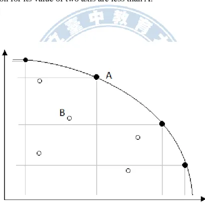
max f2(x) with 𝑓1(𝑥)ℎ𝑎𝑠 𝑏𝑒𝑒𝑛 𝑜𝑝𝑡𝑖𝑚𝑖𝑧𝑒𝑑 Eq. 2-8 3. Pareto Optimal: Without giving weight or priority for each objective, Pareto optimal
process searches whole target space to find Pareto optimal solution (or called mom-dominated solution). Pareto optimal solution is a solution set with infinite solutions and none of the set is better than any other in Pareto solution set. The basic concept is presented as follow.
19
x⃗ ≥ y⃗ and x⃗ ≠ y⃗ .
(2) x⃗ is non-dominated if ∄x⃗ ′ such that f(x⃗ ′) > f(x⃗ ).
(3) If x⃗ ∗ ∈ 𝐹 for solution field 𝐹 and x⃗ is non-dominated, then x⃗ is Pareto-optimal. (4) A Pareto-optimal set is P∗ = *x⃗ ∈ 𝐹|x⃗ 𝑖𝑠 𝑃𝑎𝑟𝑒𝑡𝑜 − 𝑜𝑝𝑡𝑖𝑚𝑎𝑙+.
For a two-objective example in Fig. 2-4, A is a Pareto-optimal solution, and B is an inferior solution for its value of two axis are less than A.
Figure 2-4 Pareto Solution
( Denotes the inferior solution; Denotes the non-inferior solution)
Recently, evolutionary algorithms such as Particle Swarm Optimization (PSO) are extended and frequently applied to solve the multi-objective problem (Coello, 2006; Mostaghim, 2003;
20
Pal, 2007). PSO represents its effective in a wide variety of applications for being able to produce excellent results without high computational cost, and having fast convergence to optimal solution (Kennedy & Eberhart, 1995). In this paper, we utilize PSO to solve the multi-objective optimization of discretization. PSO conception will be briefly introduced in the next section.
21
2.5 Particle Swarm Optimization, PSO
The particle swarm optimization (PSO) algorithm belongs to the category of swarm intelligence techniques. The swarm intelligence concepts are inspired by the social behavior of flocking animals such as swarms of birds, ants and fish school. PSO was first developed and introduced as a stochastic optimization algorithm by Eberhart and Kennedy (Kennedy & Eberhart, 1995; Lhotská, Macaš, & Burša, 2006; Wang, Sun, & Zhang, 2007). PSO is a
recently developed heuristic technique, inspired by the choreography of a bird flock. The approach can be viewed as a distributed behavioral algorithm that performs a multi-dimensional search. PSO has been found to be useful in a wide variety of optimization tasks. Due to its natural ability to converge faster, PSO algorithm is also used to solve multi-objective optimization problems.
PSO is a population-based algorithm that exploits a population of individuals to probe promising regions of the search space. The individual behavior is affected either by the best-local or best-global individual. The performance of each individual is measured using fitness function similar to evolutionary algorithms. The population is referred as a swarm and individuals are called particles. The particles move in a multi-dimensional search space with adaptable velocity. In PSO, the particles remember the best position in the past and the best
22
position ever attained by the particles. This property helps the particles to search the multi-dimensional space faster.
Let us consider an optimization problem with n-dimensional design space (Kennedy & Eberhart, 1995). Assume that there are M particles in a swarm and ith particle in a swarm is represented as a vector M i x x x Xi ( i1, i2,, in)T, 1,2,, Eq. 2-9
The velocity of the particle moving in the n-dimensional search space is
M i v v v Vi ( i1, i2,, in)T, 1,2,, Eq. 2-10
and the best position encountered by the particle is
M i b b b Bi ( i1, i2,, in)T, 1,2,, Eq. 2-11
Let us assume that the particle j attains the best position in the current iteration (l) then the position and the velocity of the particles is adapted using the following equations.
23 )) ( ) ( ( )) ( ) ( ( ) ( ) 1 (l wV l c1r1 B l X l c2r2 B l X l Vi i i i j i Eq. 2-12 ) 1 ( ) ( ) 1 (l X l V l Xi i i Eq. 2-13
where w is the inertia weight, c1, c2 represent positive acceleration constants and r1, ] 1 , 0 [ 2
r are uniformly distributed random numbers. The first term in the above equation, relates to the current velocity of the swarm, the second term represents the local search while the third term represents the global search pointing towards the optimal solution.
The inertia weight (w) is employed to control the impact of the previous history of velocities on the current velocity of each particle. Thus, the parameter w regulates the tradeoff between global and local exploration ability of the swarm. A general rule of thumb suggests that it is better to initially set the inertia to a large value, in order to make better global exploration of the search space and gradually decrease the weight to get more refined solutions. Thus, a time decreasing inertia weight value is used in this paper.
The algorithm for particle swarm optimization can be summarized as follows: Let l=1; Initialize the position and velocity of the particles in a swarm. Evaluate the performance of each particle.
24
Store the best position of each particle and best position in a swarm. WHILE the maximum number of iteration has not been reached DO. Update the velocity and position using Eqs. (2.8) and (2.9).
Maintain the particles within the search space in case they go beyond its boundaries. This condition ensures a valid solution for a given problem.
Evaluate the performance of each particle in a swarm. Store the best position of particles and swarm.
Increment the iteration loop by one, i.e., l = l + 1. END WHILE.
25
3. PROPOSED DISCRETIZATION MODEL
In this chapter, we first present our research structure of proposed discretization model in section 3.1. Multi-objective problems will be defined in section 3.2. In section 3.3, we present our proposed model with subsection 3.3.1 Notations, 3.3.2 Fitness function, 3.3.3 Pseudo code, and 3.3.4 Emulation Picture.
3.1 Research Structure
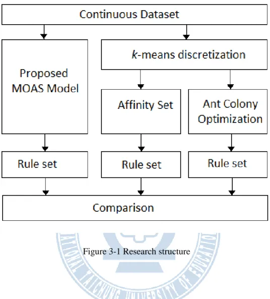
Our research attempted to compare ant colony optimization and traditional affinity set with proposed model. First, we will take a continuous data set, and discretize attributes into discrete value. After generating rule sets via those three models respectively, we compare the accuracy, number of split points, and number of rules. Research structure is presented as follow in Fig. 3-1.
26
Figure 3-1 Research structure
Notice that we use k-means to discretize the continuous dataset as contrast. Furthermore, the appropriate selection of k-core in traditional affinity set is by our determination.
27
3.2 Problem Definition
We define our problems and objectives as follows:
1. To generate appropriate number of discrete intervals: Too large number of intervals will slow down induction; on the contrary, too few intervals tend to loss information in income data. Information quality can somehow be affected by the number of intervals.
2. To maintain or improve accuracy: By constructing a supervised model, each of discretization iterations will involve accuracy condition. Sometimes information quality conflicts with accuracy.
3. To generate appropriate number of rules: Too many rules will increase the difficulty of prediction support systems construction, and too few rules oppositely lose consistency of data.
We interest in the definition ―appropriate‖ number. The simplest thought is to minimize the number of discrete intervals and number of rules; such work rather probably seems to raise accuracy. Nevertheless, we attempt to keep information without lost from original data. Assuming information is related to number of rules with a direct ratio, we should give a lower bound of the number of rules to prevent losing information.
28
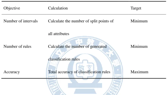
The objectives are listed as follow:
Table 3-1 Objectives of our model
Objective Calculation Target
Number of intervals Calculate the number of split points of all attributes
Minimum
Number of rules Calculate the number of generated classification rules
Minimum
Accuracy Total accuracy of classification rules Maximum
Discretization can be considered as a cut-point selecting problem of the continuous attributes. The set of k split points partitions the attribute domain into k+1 intervals that determines k+1 discrete regions. Thus we only need to calculate the number of split points. Number of rules and accuracy calculations are obvious.
29
3.3 Multi-objective Model
From previous section, we can discover that our objectives seem to be conflict between the number of intervals and rules, accuracy, and upper bound value. Therefore, a multi-objective optimization model needs to be added in the discretization process, as in the design Fig. 3-2.
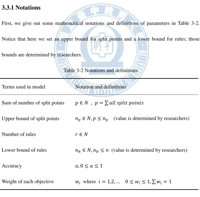
3.3.1 Notations
First, we give out some mathematical notations and definitions of parameters in Table 3-2. Notice that here we set an upper bound for split points and a lower bound for rules; those bounds are determined by researchers.
Table 3-2 Notations and definitions Terms used in model Notation and definitions
Sum of number of split points 𝑝 ∈ 𝑁 , 𝑝 = ∑ 𝑎𝑙𝑙 𝑠𝑝𝑙𝑖𝑡 𝑝𝑜𝑖𝑛𝑡𝑠
Upper bound of split points 𝑛𝑝 ∈ 𝑁, 𝑝 ≤ 𝑛𝑝 (value is determined by researchers)
Number of rules 𝑟 ∈ 𝑁
Lower bound of rules 𝑛𝑅 ∈ 𝑁, 𝑛𝑅 ≤ 𝑛 (value is determined by researchers)
Accuracy 𝑎, 0 ≤ 𝑎 ≤ 1
30
31
3.3.2 Fitness function
From the definitions and notations, here we standardize objectives into a number between 0 and 1. Besides, we alternated accuracy into error rate for finding minimum. After standardization, we have four functions and need to weight each function since we choose weight method.
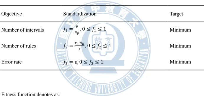
Table 3-3 Standardization
Objective Standardization Target
Number of intervals 𝑓1 = 𝑛𝑝
𝑝, 0 ≤ 𝑓1 ≤ 1 Minimum
Number of rules 𝑓2 =𝑟−𝑛r𝑅, 0 ≤ 𝑓2 ≤ 1 Minimum
Error rate 𝑓3 = 𝜀, 0 ≤ 𝑓3 ≤ 1 Minimum
Fitness function denotes as: 𝐹∗ = 𝑤
1𝑓1+ 𝑤2𝑓2+ 𝑤3𝑓3 Eq. 3-1
where 𝑤1, 𝑤2, 𝑤3 are the weight of the four objective functions
32
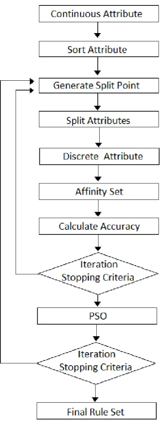
3.3.3 Pseudo code
FOR (ITERATION TIMES = 10000) {
FOR (ALL ATTRIBUTES ONE BY ONE) { //discretization
SORT;
GENERATE SPLIT POINTS (TOTAL = UPPER BOUND); FOR (ALL SPLIT POINTS) {
IF (SPLIT POINTS ARE EQUAL) { SPLIT POINTS – 1; }
}
CREATE INTERVALS; }
FOR (ITERATION TIMES = 1000) { //generate classification rules
GENERATE RULES (RANDOM NUMBER UNDER UPPER BOUND); CALCULATE ACCURACY;
}
CALCULATE FITNESS;
PSO CORRECTING SPILT POINTS POSITION; }
33
3.3.4 Emulation Picture
Step 1: Randomly select dividing points (we can set up the maximum number of bins)
Figure 3-3 randomly select dividing points
Step 2: List all possible rule set and calculate affinity degree
34
Step 3: Iterate selecting rules randomly and calculate fitness
Figure 3-5 Iterate selecting rules randomly
Step 4: select dividing bins via PSO
35
Step 5: Iterate Step 2 to Step 4, until reaching terminating conditions.
36
4. DATA ANALYSIS
In this paper we use two datasets: the well-known iris flower data set, and multiple enrollment program and academic achievements dataset attained in St. John's University. The details of the datasets are listed as in Table4-1.
Table 4-1 Details of datasets
Data set Examples Attributes Classes
IRIS flower
data set
150 Sepal length (continuous) Sepal width (continuous) Petal length (continuous) Petal width (continuous)
Setosa Versicolor Virginica Multiple enrollment dataset
460 Academic achievements average (continuous)
Physical training score (continuous)
Score rank in class (continuous) College department (discrete) Gender (discrete)
Apply for admission Screening test
Screening test (disaster area) Screening test (technique) Joint College Entrance Examination
37
IRIS flower data set was obtained from University of California at Irvine (UCI)’s data set repository, and multi enrollment dataset of multi enrollment programs in Taiwan’s technical–
vocational college was obtained from a 4-year system technical–vocational college in Taipei (personal information was removed for protecting the students’ privacy). The number of examples, attributes and classes of these data sets is shown in Table 4-2.
Table 4-2 Main characteristics of the data sets used in the experiments
Data set # examples # attributes # classes
IRIS flower data set 150 4 3
38
4.1 Experiment I: IRIS dataset
The IRIS data takes example from two characteristic marks of flowers: sepal and petal. Researchers can infer a flower’s species from its sepal length, sepal width, petal length, and petal width. Input data is numerical value; output class consists three species: Setosa, Versicolor, and Virginica.
4.1.1 Descriptive statistics
The attributes and class of IRIS data set are listed in Table 4-3. The attributes of IRIS flower data set were previously discretized into discrete values for ant colony optimization and traditional affinity set using k-means cluster, denoted as sl-1, sl-2, sl-3, sw-1, sw-2, etc. Before experiment, the parameters settings for ACO, affinity set, and proposed multi-objective affinity set are given below.
39
Table 4-3 Attributes and class coding of IRIS dataset Attributes Sepal length Average: 5.843
Standard deviation: 0.825 Sepal width Average: 3.0573
Standard deviation: 0.434 Petal length Average: 3.758
Standard deviation: 1.759 Petal width Average: 1.199
Standard deviation: 0.760 Class Species Setosa, Versicolor, Virginica
40
4.1.2 Experiment Results
Custom dividing point for ACO and Traditional Affinity Set is listed as follows: (k-means)
Table 4-4 Custom dividing point for ACO and Traditional Affinity Set Sepal length Dividing point 1: Sepal width <5.6
Dividing point 2: 5.6<= Sepal width <=6.5 Dividing point 3: Sepal width >6.5
sl-1 sl-2 sl-3
Sepal width Dividing point 1: Sepal width<2.8
Dividing point 2: 2.8<= Sepal width <=3.4 Dividing point 3: Sepal width >3.4
sw-1 sw-2 sw-3
Petal length Dividing point 1: Petal length <3
Dividing point 2: 3<= Petal length<=5.1 Dividing point 3: Petal length >5.1
pl-1 pl-2 pl-3
Petal width Dividing point 1: Petal width<1
Dividing point 2: 1<= Petal width<=1.7 Dividing point 3: Petal width>1.7
pw-1 pw-2 pw-3
41
Table 4-5 Parameters settings for experiment I
Methodology Parameters Value
Ant colony optimization Folds 10
Number of ants 10
Default class Virginica
Minimum cases per rule 5
Maximum uncovered cases 10
Rules for convergence 10
Number of iterations 100
Affinity set Selection of k 32%
Default class Virginica
Multi-objective affinity set Maximum number of rules (N) 5
Default class Virginica
42
The following presents the classification rules below and comparison results in Table 4-9. Rule set from ant colony optimization:
Table 4-6 Rule set from ant colony optimization
Rule 1 IF Petal length = pl-3
THEN Species = Setosa
Rule 2 IF Petal length = pl-1 AND PetalWidth2 = pl-3
THEN Species = Versicolor
Rule 3 IF Petal length = pl-2
THEN Species = Virginica
Rule 4 IF Sepal length = pl-1
THEN Species = Virginica
43
Rule set from multi-objective affinity set:
Table 4-7 Rule set from multi-objective affinity set
Rule 1 IF Sepal length= sl-2 AND Sepal width= sw-1 AND Petal length = pl-1
AND Petal width = pw-3
THEN Species= Versicolor
Rule 2 IF Sepal width= sw-1 AND Petal width = pw-1
THEN Species= Setosa
Rule 3 IF Petal length = pl-1 AND Petal width = pw-3
THEN Species= Versicolor
Rule 4 IF Petal width = pw-1
THEN Species= Setosa
Default Species = Virginica
From the results in Table 4-6 and Table 4-7, rule set generated by proposed model seems to contain more variety; thus, these rules keep more information and are more meaningful for botanist or biologist to analyze.
44
Table 4-8 Dividing point for multi-objective affinity set Sepal length Dividing point 1: Sepal width <5.62
Dividing point 2: 5.62<= Sepal width <=6.82 Dividing point 3: Sepal width >6.82
sl-1 sl-2 sl-3
Sepal width Dividing point 1: Sepal width <2.88
Dividing point 2: 2.88<= Sepal width <=3.68 Dividing point 3: Sepal width >3.68
sw-1 sw-2 sw-3
Petal length Dividing point 1: Petal length <3.16
Dividing point 2: 3.16<= Petal length <=5.13 Dividing point 3: Petal length >5.13
pl-1 pl-2 pl-3
Petal width Dividing point 1: Petal width <0.98
Dividing point 2: 0.98<= Petal width <=1.78 Dividing point 3: Petal width >1.78
pw-1 pw-2 pw-3
This discretization result shows that the proposed model and k-means split the continuous data with some near split points and same number of split points; which means they generate in similar quality.
45
Table 4-9 Classification results of experiment I
Algorithm Accuracy # rules
Ant colony optimization 76.67% 4
Affinity set 88.00% 6
*Multi-objective affinity set 97.33% 4
* denotes the best model
In this IRIS classification case, the result shows Multi-objective affinity set seems to be the best model among three classification methods. In the next two sections, we applied and compared the three models on practical issues for experiment.
46
4.2 Experiment II: Multiple Enrollment Dataset
The multi enrollment dataset was observed and collected from a 4-year system technical– vocational college in Taipei in 2001. In the dataset, we choose several attributes such as grade, conduct, sports, etc. to deduce the enrollment type of multi enrollment programs in Taiwan’s technical–vocational college obtained. Since the concept of Multiple Intelligence was proposed by Gardner in 1993 (Gardner, 1993), multi enrollment program became a trend of enrollment entrances program in many countries. In 1995, Taiwan Ministry of Education proposed ―The report of education in Taiwan, ROC‖ (Ministry-of-Education, 1995), paraded and planned the multi enrollment entrance program to enhance students’ learning effect and
interests by a more adapted selection. Therefore, in this case we experiment the attributes, which can easily be observed and present students’ learning effect, to examine how effectively
multi enrollment worked. The attributes and details are listed in Table 4-10. In addition, students’ personal information was removed for protecting privacy.
47
4.2.1 Descriptive statistics
Table 4-10 Attributes and class coding of IRIS dataset
Attributes Conduct Average: 87.202
Standard deviation: 5.205
Grade Average: 69.741
Standard deviation: 7.503
Sports Average: 76.780
Standard deviation: 10.749 Rank in class Average: 29.407
Standard deviation: 16.804 School Score Average: 87.202
Standard deviation: 5.205 Class Enrollment entrances Application (Application)
Joint entrance examination (Joint) Audition (Audition)
Cerebral palsy disability (Disability) Disaster area admission (Disaster) Technical admission (Tech)
48
4.1.2 Experiment Results
Custom dividing point for ACO and traditional Affinity Set
Table 4-11 Custom dividing point for ACO and traditional Affinity Set Conduct Dividing point 1: Conduct<83
Dividing point 2: 83<= Conduct<=88 Dividing point 3: Conduct>88
Low Middle High Grade Dividing point 1: Grade<65
Dividing point 2: 65<= Grade<=73 Dividing point 3: Grade>73
Low Middle High Sports Dividing point 1: Sports<47
Dividing point 2: 47<= Sports<=76 Dividing point 3: Sports>76
Low Middle High Rank in class Dividing point 1: Rank<21
Dividing point 2: 21<= Rank<=40 Dividing point 3: Rank>40
Front Middle Post School Score Dividing point 1: SchoolScore<83
Dividing point 2: 83<= SchoolScore<=88 Dividing point 3: SchoolScore>88
Low Middle High
49
Table 4-12 Parameters settings for experiment I
Methodology Parameters Value
Ant colony optimization Folds 10
Number of ants 10
Default class Joint
Minimum cases per rule 5
Maximum uncovered cases 10
Rules for convergence 10
Number of iterations 100
Affinity set Selection of k 35%
Default class Joint
Multi-objective affinity set Maximum number of rules (N) 5
Default class Application
50
The following presents the classification rules set in Table 4-13 to 4-15. The comparison result was presented in Table 4-17. Rule set from ant colony optimization:
Table 4-13 Rule set from ant colony optimization
Rule 1 IF Conduct = Middle AND Grade = Middle
THEN enrollment= Joint
Rule 2 IF Conduct = Low
THEN enrollment= Joint
Rule 3 IF ClassRank = Front
THEN enrollment= Joint
Rule 4 IF Grade = Low
THEN enrollment= Joint
Rule 5 IF Conduct = High AND Grade = High
THEN enrollment=Audition
Rule 6 IF Conduct = High AND Sports = Middle
THEN enrollment= Joint
51
Rule set from affinity set:
Table 4-14 Rule set from affinity set
Rule 1 IF Sports=Middle
THEN Enrollment= Joint
Rule 2 IF Grade= Middle
THEN Enrollment= Joint
Rule 3 IF SchoolScore= Middle
THEN Enrollment= Joint
Rule 4 IF Conduct= Middle
THEN Enrollment= Joint
Rule 5 IF Conduct= Middle AND SchoolScore= Middle
THEN Enrollment= Joint
Rule 6 IF Grade= Middle AND Sports= Middle
THEN Enrollment= Joint
Rule 7 IF Sports= Middle AND SchoolScore= Middle
THEN Enrollment= Joint
Rule 8 IF Conduct= Middle AND Sports= Middle
52
Rule 9 IF Conduct= Middle AND Sports= Middle AND SchoolScore= Middle
THEN Enrollment= Joint
Rule 10 IF ClassRank= Middle
THEN Enrollment= Joint
Default enrollment=Joint
In this multi enrollment case, we selected rules by setting k=35%, and obtained totally 10 rules; however, the k-core method cannot help us to avoid the rule set pointing to the same class, thus the rule set cannot reveal the feature of the dataset. On the contrary, our proposed multi-objective affinity set has the advantage to avoid the kind of issues happen by using iteration selection. Rule set from multi-objective affinity set is listed as follow in Table 4-15.
The proposed multi-objective affinity set output totally 4 rules, and is fewer than ACO (6 rules) and traditional affinity set (10 rules). These four rules highlight the ―School Score‖ ,an
integrated number considered attendance, bonus point by teachers, merits, and faults , might be a major attribute that shows the difference of students’ learning effects by different
53
Table 4-15 Rule set from multi-objective affinity set
Rule 1 IF SchoolScore =Low
THEN enrollment= Joint
Rule 2 IF Grade = Low AND SchoolScore =Middle
THEN enrollment= Joint
Rule 3 IF Sports = Low AND SchoolScore =High
THEN enrollment= Joint
Rule 4 IF Grade = Middle AND Sports = Low
THEN enrollment= Joint
Default enrollment=Application
Dividing points is shown in Table 4-16.
Notice that in attribute ―Conduct‖ and ―Rank in class‖ both have only one dividing point, less
54
Table 4-16 dividing point for multi-objective affinity set Conduct Dividing point 1: Conduct<95.0
Dividing point 2: Conduct>=95.0
Low High Grade Dividing point 1: Grade<49.41
Dividing point 2: 49.41<= Grade<=62.87 Dividing point 3: Grade>62.87
Low Middle High Sports Dividing point 1: Sports<23.83
Dividing point 2: 23.83<= Sports<=57.23 Dividing point 3: Sports>57.23
Low Middle High Rank in class Dividing point 1: Rank<62
Dividing point 3: Rank>=62
Front Post School Score Dividing point 1: SchoolScore<81.17
Dividing point 2: 81.17<= SchoolScore<=87.80 Dividing point 3: SchoolScore<87.80
Low Middle High
55
The following is the comparison of three models.
Table 4-17 Classification results of experiment II
Algorithm Accuracy # rules
Ant colony optimization 61.44% 6
Affinity set 61.30% 8
*Multi-objective affinity set 61.50% 4
* denotes the best model
This result shows that the proposed multi-objective affinity set has advantages to enhance accuracy, and decrease the number of split points and rules. Fewer rules without losing information and variety can be more easily applied and build for education diagnosis system.
56
5. CONCLUSION
5.1 Conclusion
The major purpose of this research is to combine multi-objective decision making and affinity set classification method, and enhance accuracy of output rule set. Since skipping the k-core method of traditional affinity set, the combination of rules has more variety to be chosen and has a higher prediction accuracy of the three experiments in this study. Furthermore, our improved multi-objective affinity set can reduce the necessary numbers of classification rules. As a result, our method improves the prediction accuracy via fewer classification rules, and makes the system based on classification rules in real world easier to be applied or constructed, such as web interface on internet, educational support software on PC, etc.
5.2 Future Works
This study focuses on increasing classification accuracy and reducing the number of dividing points and number of classification rules. Since skipping the k-core method of traditional affinity set, the combination of rules has more variety to be chosen and has a higher prediction accuracy of delayed diagnosis detection. Moreover, there are still objectives can be added to
57
the MO affinity set system, such as higher TN, lower FP, etc. On future applications, the focus of the improvement of the multi-objective model should aim at real-world problems, such as making the system more sensitive for predicting some particular attributes. For example, medical diagnosis system via observing patients’ blood pressure, body temperature, pulse, etc.,
58
REFERENCES
1. Ahmad, M. A., & Srivastava, J. (2008). An Ant Colony Optimization Approach to Expert Identification in Social Networks. Social Computing, Behavioral Modeling, and
Prediction, 120-128.
2. Barakat, N. H. (2007). Rule Extraction from Support Vector Machines: A Sequential Covering Approach. IEEE Transactions on Knowledge and Data Engineering, 19(6), 729-741.
3. Berrado, A., & Runger, G. C. (2007). Using Metarules To Organize And Group Discovered Association Rules. Data Mining and Knowledge Discovery, 14(3), 409-431. 4. Brauers, W. K. M., Zavadskas, E. K., Peldschus, F., & Turskis, Z. (2008). Multi-objective
decision-making for road design. Transport 23(3), 183 - 193.
5. Chen, Y.-W., & Larbani, M. (2007). Affinity Set and Its Applications. Paper presented at the Proceeding of the International Workshop on Multiple Criteria Decision Making, Poland.
6. Chen, Y.-W., Larbani, M., Shen, C.-M., & Chen, C.-W. (2008). Using Affinity Set on Finding the Key Attributes of Delayed Diagnosis. Applied Mathematical Sciences, 3(7), 217-316.
59
7. Chen, Y.-W., Larbani, M., Wu, C.-L., & Chen, C.-W. (2007). Using Affinity Set Theory to Enhance the Effectiveness of Head Computed Tomography.
8. Coello, M. R.-s. C. A. C. (2006). Multi-Objective particle swarm optimizers: A survey of the state-of-the-art. International Journal of Computational Intelligence Research, 2(3), 287-308.
9. Deb, K. (2001). Multi-Objective Optimization using Evolutionary Algorithms: John Wiley & Sons, England.
10. Dougherty, J., Kohavi, R., & Sahami, M. (1995). Supervised and Unsupervised
Discretization of Continuous Features. Paper presented at the Machine Learning:
Proceeding of the Twelve International Conference.
11. Gardner, H. (1993). Multiple intelligences: The theory in practice. New York: Basic Books.
12. Grzymala-Busse, J. W. (2002). Data reduction: discretization of numerical attributes. In
Handbook of data mining and knowledge discovery. New York, NY: Oxford University
Press, Inc.
13. Ho, D. Y. F. (1998). Interpersonal Relationships and Relationship Dominance: An Analysis Based on Methodological Relationism. Asian Journal of Social Psychology, 1, 1-16.
60
14. Holden, N., & Freitas, A. A. (2004). Web Page Classification with an Ant Colony Algorithm. Lecture Notes in Computer Science, 3242, 1092-1102.
15. Hwang, K.-K. (1987). Face and Favor: The Chinese Power Game. The American Journal
of Sociology, 92(4), 944-974.
16. Ishibuchi, H., Nakashima, T., & Nii, M. (2005). Multi-Objective Design of Linguistic Models. In Classification and Modeling with Linguistic Information Granules (pp. 131-141): Springer Berlin Heidelberg.
17. Jensen, R., & Shen, Q. (2006). Webpage Classification with ACO-enhanced Fuzzy-Rough
Feature Selection. Paper presented at the Proceedings of the Fifth International
Conference on Rough Sets and Current Trends in Computing (RSCTC 2006), LNAI 4259. 18. Kennedy, J., & Eberhart, R. C. (1995). Particle swarm optimization. Paper presented at
the IEEE Int. Conf. on Neural Networks, Piscataway, NJ.
19. Kerber, R. (1998). Chimerge: Discretization of numeric attributes. Paper presented at the the 10th Conference of the American Association for Artificial Intelligence.
20. Kianmehr, K., Alshalalfa, M., & Alhajj, R. (2008). Effectiveness of Fuzzy Discretization
for Class Association Rule-Based Classification. Paper presented at the Foundations of
Intelligent Systems.
61
Paper presented at the Intelligent Data Engineering and Automated Learning – IDEAL 2006.
22. Liu, H., Hussain, F., Tan, C. L., & Dash, M. (2002). Discretization: An Enabling Technique. Data Mining and Knowledge Discovery, 6(4), 393-423.
23. Luo, Y. (2000). Guanxi and Business (Vol. 1): World Scientific.
24. Mendelson, & B. (1990). Introduction to Topology. Dover Publications.
25. Ministry-of-Education. (1995). An Report of education in Taiwan, ROC o. Document Number)
26. Mostaghim, S. (2003). The Role of -dominance in Multi Objective Particle Swarm
Optimization Methods. Paper presented at the Proceedings of the 2003 Congress on
Evolutionary Computation.
27. Pal, P. K. T. S. B. S. K. (2007). Multi-Objective Particle Swarm Optimization with time variant inertia and acceleration coefficients Information Sciences, 177(22), 5033-5049 28. Pfahringer, B. (1995). Compression-Based Discretization of Continuous Attributes. Paper
presented at the Proceedings of the 12th International Conference on Machine Learning. 29. Piatrik, T., & Izquierdo, E. (2006). Image Classification Using an Ant Colony
Optimization Approach. Lecture Notes in Computer Science, 4306, 159-168.
62
Algorithm for Discretization of Continuous Attributes. In Progress in WWW Research and
Development (Vol. 4976): Springer-Verlag Berlin Heidelberg.
31. Skubacz, M., & Hollmén, J. (2008). Quantization of Continuous Input Variables for
Binary Classification. Paper presented at the Intelligent Data Engineering and Automated
Learning — IDEAL 2000. Data Mining, Financial Engineering, and Intelligent Agents. 32. Wang, Z., Sun, X., & Zhang, D. (2007). A PSO-Based Classification Rule Mining
Algorithm (Vol. 4682). Heidelberg: Springer Berlin.
33. Wu, C.-H., Lin, W.-T., Li, C.-H., Fang, I.-C., & Wu, C.-H. (2008). Ant Colony
Optimization On Building An Online Delayed Diagnosis Detection Support System For Emergency Department. Paper presented at the CIEF 2008.
34. Wu, C.-H., Lin, W.-T., Li, C.-H., Fang, I.-C., & Wu, C.-H. (2009). A Novel
Multi-Objective Affinity Set Classification System: An Investigation of Delayed Diagnosis Detection. Paper presented at the 1st Asian Conference on Intelligent Information and