利用支援向量機器預測特定位置突變所引起的蛋白質穩定性改變

國

立

交

通

大

學

生物資訊研究所

碩

士

論

文

利用支援向量機器預測特定位置突變

所引起的蛋白質穩定性改變

Prediction of thermostablity of single point mutation using the

support vector machine

研 究 生：盧 慧

指導教授：黃鎮剛 教授

利用支援向量機器預測特定位置突變

所引起的蛋白質穩定性改變

Prediction of thermostablity of single point mutation using the

support vector machine

研 究 生：盧 慧 Student：Lu Huei

指導教授：黃鎮剛 Advisor：Jenn-kang Hwang

國 立 交 通 大 學

生 物 資 訊 研 究 所

碩 士 論 文

A Thesis

Submitted to Institute of Bioinformatics

College of Biological Science and Technology

National Chiao Tung University

in partial Fulfillment of the Requirements

for the Degree of

Master

in

Bioinformatics

March 2007

Hsinchu, Taiwan, Republic of China

利用支援向量機器

預測特定位置突變所引起的蛋白質穩定性改變

學生：盧慧

指導教授：黃鎮剛

國立交通大學生物資訊研究所碩士班

摘

要

預測特定位置突變所引起的蛋白質穩定性改變是生物學上的重要議題，將

序列及結構資訊有效的轉換為能量參數，將有助於蛋白質穩定性及功能的

分析。近年來許多團隊將心力投注於單點特定位置突變及整體穩定性之實

驗數據之間關連性。在這篇論文我們利用支持向量機器預測特定位置的單

點突變所引起的蛋白質熱穩定性改變。基於前人的理論基礎，我們以八種

不同的編碼方式將結構或序列資訊轉換為特徵向量，用以測試三個經由特

定條件由線上資料庫 ProTherm 得出之公開資料集 S1615, S2048 以及

S1396，並以預測平均準確率及 Matthews 相關係數評量我們的實驗成果。

實驗數據顯示我們的方法可與目前最好的方法相當，並進一步能單以一級

序列資訊改進在相同條件下預測準確率及相關性，這在醫療科技及蛋白質

工業中缺乏次級以上結構資訊的多數情況下有實用性價值，利用本方法以

電腦計算並預測特定位置突變所引起的蛋白質穩定性改變，我們可大幅減

低傳統實驗的時間及成本。

Prediction of thermostability of single point mutation using the support

vector machine

Student:

Lu

Huei

Advisor:

Dr.

Hwang

Jenn-Kang

Institute of Bioinformatics

National Chiao Tung University

ABSTRACT

To predict the effect of site-specific mutation on protein stability and function

has been an important issue of protein science. Turning Sequence and structure

information into energetic parameters enables us to predict and analyze protein

function. In this experiment we predict the thermostability of single point

mutation using the support vector machine. Based on previous knowledge of

thermostability prediction of single point mutation, we use eight different

encodings to transform sequence information and structure information into

feature vectors to test the three public datasets extracted by certain filters from

ProTherm. We use average accuracy and Matthews correlation coefficient of

prediction of thermostability to evaluate our experiment results. The results

show that our methods are comparable with the best current methods. Further

more, we can predict the thermostability of single point mutation using the

support vector machine by sequence information only when further information

is not available yet.

誌

謝

感謝對這篇論文的產生居功厥偉的人們，感謝我的父母家人，感謝指導教

授及口試委員。感謝實驗室的學長姐跟同學，感謝親切的生科系諸位老師，

一路從管科系走到今天，引領我不遺餘力並多方鼓勵我。Thanks to Morten

Skaaning of DTU。感謝支持我的朋友。感謝教會的兄弟姊妹，感謝上帝。

Contents

Figure Contents vii

Introduction 1

Materials and Method 2

Datasets 2 Identifying thermostable and non-thermostable mutants 4

The encoding features 4

Method 1: Sequence-only Method 5

Method 2: Structure-only Method 5

Method 3: Sequence and Structure Method 6

Method 4: 6-area Method 6

Method 5: The 11win Method 7

Method 6: The di-peptide method 7

Method 7: Sequence-only with PSSM, WS =7 Method 8 Method 8: Sequence-only with PSSM, WS = 11 Method 8

The support vector machine 9

Performance measures 10

Results 10

The performance of the prediction 10

Comparison to previous work 12

Discussion 13

Comparing between different datasets 13

Classification strategy 14

Effect of eliminating redundancy data 14

Trade-offs and efficiency 14

Parameters and cross-validation 14

Conclusion 15

Tables 17

Figures 23

Table Contents

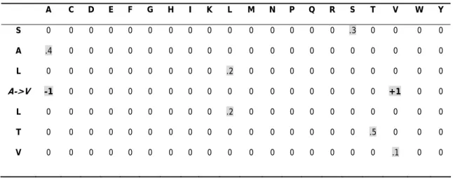
Table 1. Sequence-only Method illustration. E.g. 3SSI, AGSALALTVAGÆAGSALVLTVAG (A) with WS = 7 (B) with WS = 11.

Table 2. Performance results of different methods in different datasets. (A) S1615 (B) S2048 (C) S1396 (D) SR1496 (E) PSSM 11win Method (F) PSSM 7win Method

Table 3. The probability of residues occur both in a structural sphere of a radius of 9 angstroms and in different sequential fragments.

Table 4. The experiment results of S1396 after reducing redundancy data.

Figure Contents

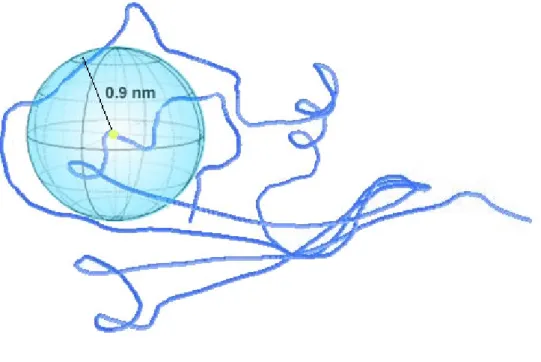
Figure 1. The Structure-Only Method illustration. To calculate the probability of occurrence of a specific amino acid within the 9 angstroms sphere centered at the Cα atom of the mutant

residue. The distances of the Cα atoms to the center are shorter than 9 angstroms.

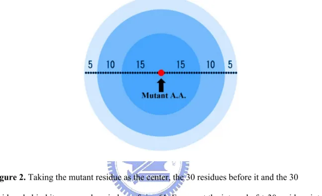
Figure 2. Taking the mutant residue as the center, the 30 residues before it and the 30 residues behind it composed a window of size 61. Fragment the interval of ± 30 residues into 6 areas, calculate the probabilities of twenty amino acids within these areas. Intervals aligning with X represents the mutation center is [ 5—10—15—X—15—10—5 ] .

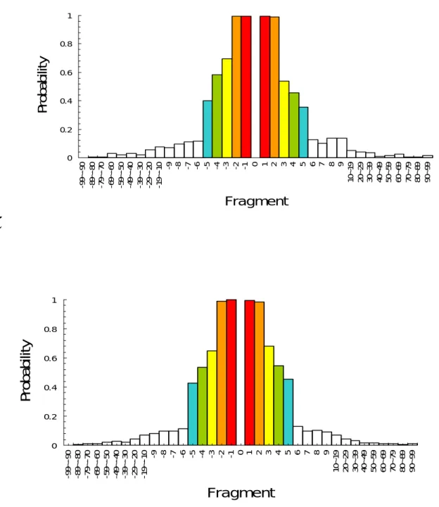
Figure 3. The probabilities distribution of residues occur in different sequence intervals and in the structural neighborhood. The structural neighborhood is defined as the distance of the Cα atom of it between the Cα atom of the mutant residue is shorter than 9 angstroms.(A)

Introduction

To predict the change of protein stability due to site-specific mutations is a long-term goal of protein science. Translation of protein sequence and structural information into energetic parameters enables us to analyze protein stability and function. For industrial and medical enzyme designing, one important requirement is the accurate prediction of protein stability changes resulting from single amino acid substitution. Hence, many efforts have been put into this field and a significant database ProTherm (Kumar, Bava et al. 2006) of the thermodynamic data on protein stability changes upon single point mutation has been generated in 1998. There are many existing approaches aimed for predicting protein stability change upon the site-specific mutation, showing the critical role of the comprehension of the rules that how single point mutation governed protein stability. For instances, using amino acid substitutions and empirical energy functions (Guerois, Nielsen et al. 2002); using knowledge based stability scale for twenty amino acid residues (Zhou and Zhou 2002); using contact potentials (Khatun, Khare et al. 2004); using solventaccessible surface area (SAS) and using proper classification of dataset by supporting information such as secondary structures and solvent accessibility of wild type residues (Saraboji, Gromiha et al. 2006); using torsion and distance potentials (Gilis and Rooman 1997) and using neural networks with SAS data (Capriotti, Fariselli et al. 2004). Capriotti’s work with S1615 dataset upon neural network method achieved an 81% accuracy with Matthews Correlation Coefficient (MCC) = 0.6 in prediction of whether a mutant is thermostable or not. Cheng utilized the support vector machine to a modified dataset of S1615, namely SR1496, obtained an accuracy

of 84.7% with MCC = 0.6 (Cheng, Randall et al. 2006). They are the significant milestones for predicting protein stability change due to site-specific mutation. The support vector machine (SVM) is a robust and convenient machine learning tool which can be used to classify extra large quantity of data. The basic idea of SVM is to use a hyperplane to separate data into two classes and get the maximum margin. With appropriate kernel functions, it can be used to solve datasets with many attributes. Based on previous knowledge of thermostability prediction of single point mutation, we use eight new encodings to transform sequence information and structure information into feature vectors to test the three public datasets extracted by Capriotti and Gromiha from ProTherm. The three datasets are denoted as S1615 (Capriotti, Fariselli et al. 2004), S2048 (Capriotti, Fariselli et al. 2005) and S1396 (Saraboji, Gromiha et al. 2006). We use average accuracy and Matthews correlation coefficient to evaluate our experiment results of prediction of thermostability. The results show that our methods are comparable with the best current methods. Furthermore, we can predict the thermostability of single point mutation using the support vector machine by sequence information only when further information is not available yet.

.

Materials and Method

Datasets

In order to compare the performance with previous works with identical inputs, we use published datasets. The three datasets were extracted from ProTherm. ProTherm is an online database of collection of numerical data of thermodynamic parameters of wild type and

mutant proteins such as Gibbs free energy change, enthalpy change, heat capacity change, and transition temperature. Dataset S1615 includes 1615 single mutations obtained from 42 different proteins. The three filters of retrieving data from ProTherm of S1615 are : 1. The

value of the mutant protein has been experimentally detected and is reported in the databases. 2. The data are relative to single mutations (no multiple mutations have been taken into account). 3. The protein structure is known with atomic resolution and deposited in the Protein Data Bank (Berman, Westbrook et al. 2000). We extract the FASTA files and structural files from Protein Data Bank (PDB) of all mutants in S1615. Some of the PDB codes need to be corrected manually for some entries were replaced by new PDB codes. The original dataset is available at

G ΔΔ

http://www.biocomp.unibo.it/piero/ddgp.Dataset 2048 includes 2048 single mutations obtained from 64 different proteins. The two filters of retrieving data from ProTherm of S2048 are : 1. The ΔΔG value has been experimentally detected and is

reported in the databases. 2. The data are relative to single mutations (no multiple mutations have been taken into account. We extract the FASTA files and structural files from PDB of all mutants in S2048. Some of the PDB codes need to be corrected manually for some entries were replaced by new PDB code. The original dataset is available at

http://gpcr2.biocomp.unibo.it/~emidio/I-mutant2.0/dbMutSeq.html. S1396 includes 1396 single mutations obtained from 48 different proteins. The three filters of retrieving dataset from ProTherm of S1396 are : 1. The data are relative to single mutations (no multiple mutations have been taken into account). 2. Containing secondary structure and SAS (Ooi, Oobatake et al. 1987) information. 3. Containing experimental free energy change. We extract the FASTA files and structural files from PDB according to the PDB codes of all mutants in S1396. Some of the PDB codes need to be corrected for entries were replaced by new PDB codes. The original dataset is available at http://www.interscience.wiley.com/jpages/ 0006-3525/suppmat.

Identifying thermostable and non-thermostable mutant

The protein unfolding free energyΔΔG(kJ/mol)is the difference of free energy ΔG

between wild type and mutant type protein. The free energy is negative when a chemical reaction occurs spontaneously. The more negative ΔG is, the more likely the chemical

reaction will occur for every system seeks to achieve a minimum of free energy. When assigning the attribute values, we follow the rule built by Capriotti (Capriotti, Fariselli et al. 2004) : If the change of free energy, ΔΔG, is negative, then the mutation decreased the

protein stability and is classified as a “unstablizing” mutation, desired output set to 0. If the change of free energy, , is positive, then the mutation increased the protein stability and is classified as a “stabilizing” mutation, desired output set to 1.

G ΔΔ

The encoding features

To build the SVM encode plausibly, we have to consider the plausible window size. Window size (Capriotti, Fariselli et al. 2005) is a fragment of protein sequence that centered at the residue that undergoes the mutation and that symmetrically spans the sequence to the left (N-terminus) and to the right (C-terminus) with variable lengths

.

atoms of residues. We use the Position-Specific Scoring Matrix information for encoding. Position-Specific Scoring Matrix (PSSM) gives the log-odds score for finding a particular matching amino acid in a target sequence.

Method 1: Sequence-only Method

Sequence-only Method (SO Method) takes the single mutant residue as the center, and takes the three residues before it and the three residues behind it to compose a window of size seven. Therefore the window size (WS) = 2n + 1, n = 3. Hence, the possibilities of the combination of seven specific residues showing in a specific sequence form a 7×20

matrix. Calculate the probability of the occurrences of a specific residue over all the amino acids occurred in the dataset itself; we have twenty values of probability ranged from 0 to 1. For example, the probability of occurrence of Alanine over all the amino acids in S1396 is 0.79. If Alanine shows within the window, it will be assigned a value of 0.79. After encoding the total 140 vectors in the form of probability value into attributes (Illustrated in Table 1A), we use LIBSVM build-in module to select the best SVM parameters.

Method 2: Structure-only Method

Structure-only Method (TO Method) takes the Cα atom of the single mutant residue as

the center of a radius of nine angstroms and calculate the probability of encountering C-alpha atoms of other residues in the sphere. The probability is calculated by the following equation: ) ( ) X ( ) ( sphere the within showing C of number total sphere the within showing of C of number the X Frequency α α =

Occurrences of a specific residue over all the residues encountered in the sphere were used to calculate the attribute value. For example, if there is one Alanine over other twelve residues encountered in a sphere, the attribute value is set to one twelfths. If one of the twenty amino acids is not encountered in the sphere, the attribute value is set to zero. The mutant center was encoded in twenty vectors in presentation of twenty amino acids. The initial values were set to 0 and using a -1 in presentation of a silent residue and a +1 as a mutated residue. Hence we encode a total forty vectors in this method (Figure 1). We use LIBSVM module to get the best SVM parameters.

Method 3: Sequence and Structure Method

Sequence and Structure Method (SOTO Method) is the combination of Method 1 and Method 2, simply add vectors together to get a total 140 + 40 = 180 vectors. After encoding, we use LIBSVM module to get the best SVM parameters.

Method 4: 6-area Method

Taking the single mutant residue as the center, together with the 30 residues before it and the 30 residues behind it, to compose a window of size 61 ( WS = 2n + 1, n=30 ). Fragment the window into six intervals of different lengths. The method is illustrated in Figure 2. We calculate the proportion of one amino acid within it’s own interval. For example, if there is one Alanine over fifteen other residues encountered in the interval, the attribute value represent the residue will be set to one fifteenths. We have six intervals coded with the twenty amino acids probability within each of them. To represent the mutant center, we add another twenty vectors. The twenty initial values were set to zero,

take value -1 in presentation of a wild residue and value +1 in presentation of a mutated residue. We encode total 120 + 20 = 140 vectors in this method.

Method 5: The 11win Method

We calculated the probability of a residue showing in a nine angstroms sphere centered in the mutant residue. For example, in dataset S1615, in the sequence interval of

29 ~

20 +

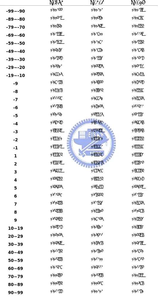
+ of one single mutant protein, the probability of Alanine shows both in the sequence interval and the structural sphere is 5.42%. We can view the relationship between sequence neighbors and structure neighbors as the relationship between sequence fragments and probability distribution. The probability of a residue shows in structural distance less than nine angstroms and a particular sequence interval at the same time is more than 95% in sequence interval ± 1 ~ ± 2, 45~65% in sequence interval ± 3 ~ ± 5, less than 20% in sequence interval ± 6 ~ ± 30, others are randomly distributed (Table 3). The 11win Method is illustrated in Table 1B. The SO method uses only the residues within the ± 3 range. We extend it into ± 5 to acquire more information. Take the mutant residue as the center, in a window of size eleven ( WS = 2n + 1, n = 5 ), we can get a 20 × 11 matrix. The probability of a specific residue showing in the dataset itself is generated to be the attribute value. We encode 220 vectors in this method. The probabilities distribution of the three datasets are shown in Figure 3.

Method 6: The di-peptide method

The Di-peptide Method (The DipepX Method) replaces the single residues by di-peptide unit. A 20 × 20 “di-peptide” matrix is generated for assigning the attribute values.

Calculate the proportion of one specific “di-peptide” in the ± 30 interval of a single mutation over all the “di-peptides” in the dataset itself, and keep the information of single Wild/Mutant site into the twenty vectors as we previously introduced in SO method, there are 420 vectors in total in The DipepX method.

Method 7: Sequence-only with PSSM, WS =7 Method

Sequence-only with PSSM, WS =7 Method (The PSSM 7win Method) takes the single mutant residue as the center, the three residues before it and the three residues behind to compose a window of size seven ( WS = 2n + 1, n = 3 ). To show the composition of specific residues in a specific position, there are 20 × 7 possible combinations. Using PSSM profiles constructed by psi-blast, we encode 140 vectors in the form of PSSM probability in this method. Adding another twenty vectors in presentation of single Wild/Mutant site by value -1 and 1 as previously introduced, we encode a total of 140 + 20= 160 vectors in this method.

Method 8: Sequence-only with PSSM, WS = 11 Method

Sequence-only with PSSM, WS = 11 Method ( The PSSM 11win Method ) takes the single mutant residue as the center, in a window of size eleven ( WS =2n + 1, n = 5 ). There are 20 × 11 possible ways of showing a specific residue in a specific position. Adding another twenty vectors in presentation of single Wild/Mutant site by value -1 and 1 as previously introduced, we encode a total of 220 + 20 vectors in this method.

The support vector machine

The support vector machine (SVM) is a binary classifier used especially when encountering a large dataset. The basic idea of SVM is to use a hyperplane to separate data points into two classes to achieve the maximum margin.If we have data points of the form:

{( X1,C1 ), ( X2,C2 ) , ( X3,C3 ) , … ,( Xn,Cn )}

where the Ci is either 1 or −1.

The constant Ci denotes the class of a point Xi belongs to. Each Xi is a real vector, usually of

values scaled to [ 0 , 1 ] or [ -1 , 1 ]. In the hyperplanewX − b=0, the vector w is

perpendicular to the plane, and the parameter b allows us to adjust the maximum margin. The hyperplane is forced to pass through the origin if parameter b is set to zero. The training data creates a hyperplane, which denotes the correct classification we would like the SVM classifier to distinguish eventually. In order to get the maximum margin of a classification of a dataset, we evaluated the plausible support vectors. The support vectors support the machine to judge their distance to the hyperplane. The parallel hyperplanes to the optimal hyperplane can be described by equations:

1 = − b wX 1 − = − b wX

If the training data are linearly separable, we can select these hyperplanes so that there are no points between them and then try to maximize their distance. The distance between the hyperplanes is 2/|w|, so we want to minimize |w|. We adapt LIBSVM 2.82 built by Chih-Jen Lin ( http://www.csie.ntu.edu.tw/~cjlin/LIBSVM/ ) to perform all the experiments. The kernel function is the radial basis function (RBF). Before executing SVM, the dataset was divided into twenty folds according to its Protein Data Bank ID order for the 20 x cross-validation. Before the optimal parameters were generated, the dataset were pre-classified by the build-in

cross-validation function to ensure the parameters are in the plausible range for providing a standard of advanced optimization. The data points were scaled into the range of [-1 , +1], for larger variances sometimes dominate the classification and cause bias.

Performance measures

The performance is measured by the average accuracy and the average Matthews correlation coefficient (Baldi, Brunak et al. 2000). Matthews Correlation Coefficient (MCC) is defined by the following equation:

) )( )( )( ( ) )( ( ) )( ( FN TN FP TN FN TP FP TP FN FP TN TP MCC + + + + − =

TP is the number of true positives, TN is the number of true negatives, FP is the number of false positives, and FN is the number of false negatives. The Matthews correlation coefficient has the advantage that it is independent of the choice of threshold. Accuracy (ACC) is defined by the following equation:

TN FN FP TP TN TP Accuracy + + + + = × 100%

Results

We measured the prediction performance by average accuracy and Matthews correlation coefficient of eight different methods. The results are shown in Table 2. Prediction of thermostability ( ΔΔG ) using The 11win method performs better (average accuracy of

dataset S2048, The 11win method performs better (average accuracy of 85.3%, the average accuracy of Cheng’s result is 85.1%). Moreover, we use sequence information only, while previous works use both sequence and structural information. We find that the prediction accuracy obtained using sequence alone is comparable to the accuracy obtained using both sequence and structural information.

The Performance of the prediction

A. Performance of methods using sequence information

The average prediction accuracy achieves as high as 86.50% with MCC=0.6487 with The 11win Method in S1615. The overall prediction accuracy achieves as high as 85.15% with MCC=0.6378 with The 11win Method in S2048. The overall prediction accuracy achieves as high as 86.83% with MCC=0.7780 with SO Method in S1396.

B. Performance of methods using sequence and structure information

The overall prediction achieves 86.6% accuracy with MCC=0.643 by SOTO Method in S1615. The reported highest prediction rate is currently 81% (Capriotti, Fariselli et al. 2004). The overall prediction achieves 85.8% accuracy with MCC=0.652 by SOTO Method in S2048. The reported highest prediction rate currently is 77%(Capriotti, Fariselli et al. 2005). The overall average prediction accuracy achieves as high as 86.83%, MCC=0.7780 with SO Method in S1396. The reported highest prediction rate currently is 85.5%(Saraboji, Gromiha et al. 2006).

C. Performance of methods using PSSM information

We use PSSM information on the three datasets and the result of prediction power was not as high as other methods (85.6% of average accuracy with MCC=0.630 by The PSSM 7win Method in S1615). However, the results are consistent with three important observations: First, S1615 is the most distinguishing dataset among the three datasets. Second, with sequence information only, WS = 7 is better than WS = 11 in the three datasets, in both accuracy and MCC value, which is also consistent with previous study of Capriotti. Third, with PSSM information, the average standard deviation of prediction accuracy (0.006) and average standard deviation of MCC (0.012) were highly reduced in WS = 7 than in WS = 11. (Table. 2E, 2F)

Comparison to previous work

The reported highest prediction rate currently is 85~86%, MCC= 0.6on S1615 (Cheng, Randall et al. 2006), our overall prediction achieves 86.6% accuracy with MCC=0.643 by SOTO Method. The reported highest prediction rate on S2048 is 77% (Capriotti, Fariselli et al. 2005).Our overall prediction achieves an 85.8% accuracy, with MCC=0.652 in S2048.The reported highest prediction rate currently is 85.5% on S1396 (Saraboji, Gromiha et al. 2006). Our overall prediction achieves 84.6626% accuracy, with MCC=0.6728 in S1396.

Discussion

In this section we are going to discuss the difference between datasets, the classification strategy, the effect of eliminating redundancy data, trade-offs and efficiency of information included in SVM coding, the parameters choosing and cross-validation strategy.

Comparing between different datasets

By comparing the experiment results (Table 2), we can find that combination of structural and sequence information can improve the performance of prediction accuracy. PSSM information was useful under sequence-only encoding feature. Using SVM, this work is robust and comparable with recent work using different approaches, under the same experimental condition. S1615 has the best distinguishing power and the least deviation from method to method. Seven out of the eight best prediction accuracy rate come from S1615 dataset. S1615 has the least standard deviations of the prediction accuracy of the three datasets.

We achieved the highest MCC value of 0.649 in S1615 by The 11win Method among all current works. The best performance within one dataset was boxed in Table 2. With our modifications, SO Method, TO Method and SOTO Method have better performances on the three datasets, better than Cheng did with their published dataset SR1496 (Table 2D). Compare the sequence information only methodz (all methods but TO Method and SOTO Method), the best yielding is the 11 Win Method in S1615, S2048, and the SO Method in

S1396.

By calculating the probability of occurrence of a specific residue both in the structural and sequence neighborhood, we find that over 95% of the nearest neighbors of the mutant center also shown in the nine-angstroms-sphere. The probability of a residue showing in structural radius less than nine angstroms in sequence position 1± and 2± is 99.7% in average.

Classification strategy

The classification of stable mutants and non-stable mutants is intuitive; due to the uneven distribution of data, the dataset can not be equally classified in any other way. We believe that the rate of 86% is so far the most possible achievement in those datasets. Since the correct prediction of the direction of the stability change is more relevant than its magnitude.

Effect of eliminating redundancy data

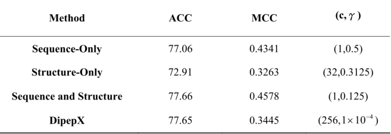
In order to reduce the effect of repeated experiments on the same position of same protein, we manually removed the same mutation in the same position and left the first one as the representing data. Hence we got a dataset of 846 mutants from S1396 (Table 4). Compared to Table 2C, the effect of eliminating redundancy data is to reduce the prediction accuracy and MCC value.

Trade-offs and efficiency

vectors of

numbers Accuracy efficiency=

Hence TO methods are highly efficient since they can reach 97% average accuracy of the best of the other methods while using only 20% the number of vectors. This fact also implies the difficulty in the task of prediction without structural information available yet.

Parameters and cross-validation

We choose SVM as the classifier for it is robust especially on large datasets. With careful optimization of parameters, the prediction accuracy can be raised significantly. We did the pre-experiment using build-in SVM cross-validation function in order to increase the fidelity of the parameter value. We then divide the data into 20 folds and fix the partition fold in each experiment. The 20 folds were divided according to the PDB ID order. Hence the partition is repeatable and the experiment results are reproducible under the same conditions.

Conclusion

The prediction accuracy obtained by us using sequence alone is comparable to the accuracy obtained using both sequence and structural information by previous works. The advantage of our methods is the capability of predicting the stability of proteins using sequence information only while other information is not available yet due to the limited resource of discovering the protein structure. From the experiments we know that the two

most important variables of sequence-only encoding are the mutation residue itself and the residue composition of vicinity. The conclusion corresponds to the previous research and if we can use structural information in the future, the performance might still be improvable.

Tables

Table 1A. Sequence-only Method with window size = 7.

A C D E F G H I K L M N P Q R S T V W Y S 0 0 0 0 0 0 0 0 0 0 0 0 0 0 0 .3 0 0 0 0 A .4 0 0 0 0 0 0 0 0 0 0 0 0 0 0 0 0 0 0 0 L 0 0 0 0 0 0 0 0 0 .2 0 0 0 0 0 0 0 0 0 0 A->V -1 0 0 0 0 0 0 0 0 0 0 0 0 0 0 0 0 +1 0 0 L 0 0 0 0 0 0 0 0 0 .2 0 0 0 0 0 0 0 0 0 0 T 0 0 0 0 0 0 0 0 0 0 0 0 0 0 0 0 .5 0 0 0 V 0 0 0 0 0 0 0 0 0 0 0 0 0 0 0 0 0 .1 0 0

Table 1B. Sequence-only Method with window size = 11. A C D E F G H I K L M N P Q R S T V W Y A .4 0 0 0 0 0 0 0 0 0 0 0 0 0 0 0 0 0 0 0 G 0 0 0 0 0 .2 0 0 0 0 0 0 0 0 0 0 0 0 0 0 S 0 0 0 0 0 0 0 0 0 0 0 0 0 0 0 .3 0 0 0 0 A .4 0 0 0 0 0 0 0 0 0 0 0 0 0 0 0 0 0 0 0 L 0 0 0 0 0 0 0 0 0 .2 0 0 0 0 0 0 0 0 0 0 A>V -1 _{0 0 0 0 0 0 0 0 0 0 0 0 0 0 0 0} +1 _{0 0} L 0 0 0 0 0 0 0 0 0 .2 0 0 0 0 0 0 0 0 0 0 T 0 0 0 0 0 0 0 0 0 0 0 0 0 0 0 0 .5 0 0 0 V 0 0 0 0 0 0 0 0 0 0 0 0 0 0 0 0 0 .1 0 0 A .4 0 0 0 0 0 0 0 0 0 0 0 0 0 0 0 0 0 0 0 G 0 0 0 0 0 .2 0 0 0 0 0 0 0 0 0 0 0 0 0 0

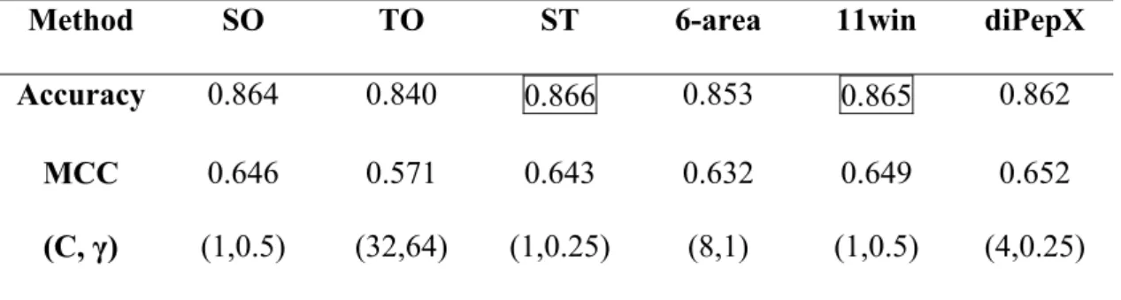
Table 2. The performance of different methods A.S1615

Method SO TO ST 6-area 11win diPepX

Accuracy 0.864 0.840 0.866 0.853 0.865 0.862

MCC 0.646 0.571 0.643 0.632 0.649 0.652

(C, γ) (1,0.5) (32,64) (1,0.25) (8,1) (1,0.5) (4,0.25) Average standard deviation of prediction accuracy =0.0078

Average standard deviation of MCC =0.0204

B.S2048

Method SO TO ST 6-area 11win diPepX

Accuracy 0.851 0.825 0.858 0.843 0.853 0.847

MCC 0.639 0.564 0.652 0.616 0.639 0.635

(C, γ) (4,0.25) (1,64) (1,0.25) (4,0.25) _{(1,0.5) (64,1.5625×10}−3₎

Average standard deviation of prediction accuracy =0.0081 Average standard deviation of MCC =0.0228

C.S1396

Method SO TO ST 6-area 11win diPepX

Accuracy 0.868 0.826 0.861 0.819 0.841 0.847

MCC 0.778 0.721 0.725 0.651 0.662 0.673

(C, γ) (16,0) (1,64) (4,0.25) (2,1) (2,0.5) (1,0.5) Average standard deviation of prediction accuracy =0.015

D.SR1496 (Cheng, Randall et al. 2006)

Method SO TO ST

Accuracy 0.841 0.845 0.847

MCC 0.59 0.6 0.6

(C, γ) N/A N/A N/A

Average standard deviation of prediction accuracy =0.0022 Average standard deviation of MCC =0.0044

E. PSSM 11win Method

Dataset S1615 S2048 S1396

Accuracy 0.854 0.850 0.822

MCC 0.627 0.629 0.563

(C, γ) (2,0.5) (1,0.5) (1,0.5) Average standard deviation of prediction accuracy =0.013 Average standard deviation of MCC =0.029

F. PSSM 7win Method

Dataset S1615 S2048 S1396

Accuracy 0.856 0.851 0.839

MCC 0.630 0.634 0.660

(C, γ) (2,0.5) (1,0.5) (2,0.25) Average standard deviation of prediction accuracy =0.006 Average standard deviation of MCC =0.012.

SO: Sequence-only Method, TO: Structure Only Method, ST: SO Method combine TO Method, 6-area: 6-area Method, 11win: 11win Method, diPepX: Dipeptide Method, PSSM 11win: SO Method, but uses PSSM information and WS = 11, PSSM 7 win: SO Method, but use PSSM information and WS = 7

Table 3. The probability of residues occur both in a radius of 0.9 nm and in different sequential fragments. S1396 S1615 S2048 -99~-90 0.00244 0.00202 0.00269 -89~-80 0.00429 0.00480 0.00767 -79~-70 0.00630 0.00539 0.00994 -69~-60 0.02969 0.02700 0.01259 -59~-50 0.01979 0.02072 0.01963 -49~-40 0.03061 0.02780 0.02756 -39~-30 0.01848 0.02961 0.02428 -29~-20 0.05502 0.04385 0.04291 -19~-10 0.07705 0.04835 0.07095 -9 0.07286 0.05644 0.08148 -8 0.09516 0.06613 0.09947 -7 0.11147 0.07750 0.09735 -6 0.11636 0.08045 0.11322 -5 0.40130 0.49915 0.42962 -4 0.58238 0.62552 0.53756 -3 0.69439 0.74389 0.64656 -2 0.99510 0.99620 0.98994 -1 0.99619 0.99772 0.99947 1 0.99673 0.99747 0.99682 2 0.98749 0.99326 0.98624 3 0.53779 0.78517 0.67883 4 0.45894 0.68913 0.54708 5 0.35345 0.59098 0.45449 6 0.12452 0.16343 0.12962 7 0.10386 0.12931 0.09735 8 0.13866 0.09604 0.10476 9 0.13594 0.07245 0.08941 10~19 0.04828 0.05602 0.06862 20~29 0.04045 0.05421 0.04396 30~39 0.03539 0.06516 0.03169 40~49 0.01163 0.01604 0.01740 50~59 0.01386 0.01200 0.01714 60~69 0.02327 0.03112 0.01164 70~79 0.00364 0.01486 0.00899 80~89 0.00483 0.00417 0.00576 90~99 0.01288 0.00202 0.01280

Table 4. The performance of S1396 after reducing redundancy data.

Method ACC MCC (c,γ)

Sequence-Only 77.06 0.4341 (1,0.5)

Structure-Only 72.91 0.3263 (32,0.3125)

Sequence and Structure 77.66 0.4578 (1,0.125)

DipepX 77.65 0.3445 (256,_1×10−4)

ACC= accuracy

MCC=Matthews correlation coefficient (c,γ) = the support vector machine parameters

Figure 1. The Structure-Only Method illustration. To calculate the probability of occurrence of a specific amino acid within the 9 angstroms sphere centered at the Cα atom of the mutant

Figure 2. Taking the mutant residue as the center, the 30 residues before it and the 30

residues behind it composed a window of size 61. Fragment the interval of ± 30 residues into 6 areas, calculate the probabilities of twenty amino acids within these areas. Intervals aligning with X represents the mutation center is [ 5—10—15—X—15—10—5 ] .

(A) 0 0.2 0.4 0.6 0.8 1 -99~ -90 -89~ -80 -79~ -70 -69~ -60 -59~ -50 -49~ -40 -39~ -30 -29~ -20 -19~ -10 -9 -8 -7 -6 -5 -4 -3 -2 -1 0 1 2 3 4 5 6 7 8 9 10 ~ 19 20 ~ 29 30 ~ 39 40 ~ 49 50 ~ 59 60 ~ 69 70 ~ 79 80 ~ 89 90 ~ 99 Fragment Pr ob ab ilit y 0 0.2 0.4 0.6 0.8 1 -99~ -90 -89~ -80 -79~ -70 -69~ -60 -59~ -50 -49~ -40 -39~ -30 -29~ -20 -19~ -10 -9 -8 -7 -6 -5 -4 -3 -2 -1 0 1 2 3 4 5 6 7 8 9 10 ~ 19 20 ~ 29 30 ~ 39 40 ~ 49 50 ~ 59 60 ~ 69 70 ~ 79 80 ~ 89 90 ~ 99 Fragment Pr ob ab ilit y (B)

Figure 3. The probabilities distribution of residues occur in different sequence intervals and in the structural neighborhood. The structural neighborhood is defined as the distance of the Cα atom of it between the Cα atom of the mutant residue is shorter than 9 angstroms.(A)

0 0.2 0.4 0.6 0.8 1 -9 9~ -90 -8 9~ -8 0 -79~ -7 0 -6 9 ~ -6 0 -5 9~ -5 0 -49 ~ -4 0 -3 9~ -3 0 -2 9~ -20 -1 9~ -1 0 -9 -8 -7 -6 -5 -4 -3 -2 -1 0 1 2 3 4 5 6 7 8 9 10 ~ 19 20 ~ 29 30 ~ 39 40 ~ 49 50 ~ 59 60~ 69 70 ~ 79 80~ 89 90 ~ 99 Fragment Pr ob ab ilit y (C)

References

Baldi, P., S. Brunak, et al. (2000). "Assessing the accuracy of prediction algorithms for classification: an overview." Bioinformatics 16(5): 412-24.

Berman, H. M., J. Westbrook, et al. (2000). "The Protein Data Bank." Nucleic Acids Res 28(1): 235-42.

Capriotti, E., P. Fariselli, et al. (2005). "Predicting protein stability changes from sequences using support vector machines." Bioinformatics 21 Suppl 2: ii54-ii58.

Capriotti, E., P. Fariselli, et al. (2004). "A neural-network-based method for predicting protein stability changes upon single point mutations." Bioinformatics 20 Suppl 1: I63-I68.

Cheng, J., A. Randall, et al. (2006). "Prediction of protein stability changes for single-site mutations using support vector machines." Proteins 62(4): 1125-32.

.

Gilis, D. and M. Rooman (1997). "Predicting protein stability changes upon mutation using database-derived potentials: solvent accessibility determines the importance of local versus non-local interactions along the sequence." J Mol Biol 272(2): 276-90.

Guerois, R., J. E. Nielsen, et al. (2002). "Predicting changes in the stability of proteins and protein complexes: a study of more than 1000 mutations." J Mol Biol 320(2): 369-87.

Khatun, J., S. D. Khare, et al. (2004). "Can contact potentials reliably predict stability of proteins?" J Mol Biol 336(5): 1223-38.

Kumar, M. D., K. A. Bava, et al. (2006). "ProTherm and ProNIT: thermodynamic databases for proteins and protein-nucleic acid interactions." Nucleic Acids Res 34(Database issue): D204-6.

Ooi, T., M. Oobatake, et al. (1987). "Accessible surface areas as a measure of the thermodynamic parameters of hydration of peptides." Proc Natl Acad Sci U S A 84(10): 3086-90.

Saraboji, K., M. M. Gromiha, et al. (2006). "Average assignment method for predicting the stability of protein mutants." Biopolymers 82(1): 80-92.

Zhou, H. and Y. Zhou (2002). "Distance-scaled, finite ideal-gas reference state improves structure-derived potentials of mean force for structure selection and stability prediction." Protein Sci 11(11): 2714-26.