國 立 交 通 大 學
電 機 與 控 制 工 程 研 究 所
碩 士 論 文
快速輻射半徑基底函數網路演算法
於蛋白質相對溶劑可接觸性預測的應用
Applying Quick Radial Basis Function Network
to Protein Relative Solvent Accessibility Prediction
學 生: 游 涵 任
指 導 教 授: 張 志 永
快速輻射半徑基底函數網路演算法
於蛋白質相對溶劑可接觸性預測的應用
Applying Quick Radial Basis Function Network
to Protein Relative Solvent Accessibility Prediction
學 生 : 游涵任 Student : Han-Jen Yu
指導教授 : 張志永 Advisor : Jyh-Yeong Chang
國立交通大學
電機與控制工程學系
碩士論文
A Thesis
Submitted to Department of Electrical and Control Engineering
College of Electrical Engineering and Computer Science
National Chiao Tung University
in Partial Fulfillment of the Requirements
for the Degree of Master in
Electrical and Control Engineering
July 2006
Hsinchu, Taiwan, Republic of China
快速輻射半徑基底函數網路演算法
於蛋白質相對溶劑可接觸性預測的應用
學生:游涵任 指導教授:張志永博士 國立交通大學電機與控制工程研究所摘要
蛋白質在生物體中一直扮演著很重要的角色,蛋白質被發現的數量及其結構 逐年增加。隨著蛋白質的應用越來越廣泛,待解決的課題也就越來越多。例如: 蛋白質二級結構預測問題、蛋白質相對溶劑可接觸性預測問題等。目前在蛋白質 結構問題的解決上,科學家都是利用X光繞射以及核磁共振 (NMR) 來取得實驗結 果。這些方法雖然正確率高,但是相對地所要花費的時間及成本是相當高的。因 此利用電腦科學中的機器學習 (Machine learning) 演算法來預測這些問題,相 信能夠有效降低實驗與時間成本。 本篇論文,我們利用修改的快速輻射半徑基底函數網路演算法,混合從 PSI-BLAST 產生的位置加權矩陣,針對蛋白質相對溶劑可接觸性預測問題進行研 究。最近歐等人 [10],發展出快速輻射半徑基底函數網路演算法,是一種較快 速且精確設計之網路,應用於蛋白質二級結構預測有顯著的效果。我們的修改的快速輻射半徑基底函數網路演算法,應用於蛋白質相對溶劑可接觸性預測。我們 使用五種不同的快速輻射半徑基底函數網路演算法,應用在三態相對溶劑可接觸 性預測和二態相對溶劑可接觸性預測。此五種方法包括:(1) 快速輻射半徑基底 函數網路演算法、(2) 二階快速輻射半徑基底函數網路演算法、(3) 一般混合快 速輻射半徑基底函數網路演算法、(4) 地域趨勢混合快速輻射半徑基底函數網路 演算法、以及(5) 全域趨勢混合快速輻射半徑基底函數網路演算法。我們選擇有 最佳表現的一般混合快速輻射半徑基底函數網路演算法,做為建議的演算法。我 們也將修改的快速輻射半徑基底函數網路演算法的實驗結果,與近幾年的其他方 法比較,並且提出我們的方法改進方向的建議。
Applying Quick Radial Basis Function Network to
Protein Relative Solvent Accessibility Prediction
STUDENT: HAN-JEN YU ADVISOR: JYH-YEONG CHANG
Institute of Electrical and Control Engineering
National Chiao-Tung University
Abstract
Proteins have been played an important role in a creature and the numbers of
proteins and their structures have been increased with years. Since protein
applications are more widely used, there will be a lot of problems to be solved. For
example, there are protein secondary structure prediction problem, protein relative
solvent accessibility problem and so on. Nowadays, scientists use X-ray diffraction or
nuclear magnetic resonance (NMR) to solve the protein structure problem. Although
they can achieve high accuracy, it is expensive and long to solve this protein problem.
To reduce the time and the costs, it is imperative to use machine learning algorithms
to solve this protein problem.
In this thesis, we study protein relative solvent accessibility problem using a
modified QuickRBF method combined with a position-specific scoring matrix (PSSM)
generated from PSI-BLAST. The QuickRBF method, recently developed by Ou et al.
[10], has been applied to protein secondary structure prediction with excellent results.
Our modified QuickRBF method is applied on relative solvent accessibility prediction.
Five different kind of QuickRBF approaches are applied on three-state, E, I, and B,
and two-state, E, and B, relative solvent accessibility predictions. These five
approaches include: (1) QuickRBF, (2) Two-Stage QuickRBF, (3) Common Fusion
QuickRBF, (4) Local Tendency Fusion QuickRBF, and (5) Global Tendency Fusion
QuickRBF. We recommend the Common Fusion QuickRBF approach which has the
best performance as our modified QuickRBF method. We also compare the results of
the modified QuickRBF method with other methods in the recent years, and suggest
Acknowledgement
I would like to express my sincere appreciation to my advisor, Dr. Jyh-Yeong
Chang. Without his patient guidance and inspiration during the two years, it is
impossible for me to overcome the obstacles and complete the thesis. In addition, I am
thankful to all my lab members for their discussion and suggestion.
Finally, I would like to express my deepest gratitude to my family. Without their
Contents
Abstract (Chinese)…………..………..3 Abstract (English).………...……….5 Acknowledgement………..………..7 List of Figures………..………...…10 List of Tables………..………...11 Chapter 1. Introduction………..………..121.1 Motivation and The Background of This Research………12
1.2 Thesis Outline……….…...13
Chapter 2. Materials and Methods……….….…14
2.1 Training and Data Set………..14
2.2 Definition of Solvent Accessibility……….………...…....16
2.2.1 Static Residue Solvent Accessibility………..16
2.2.2 Residue Relative Solvent Accessibility………..18
2.3 PSI-BLAST Profiles………22
2.4 Quick Radial Basis Function Network…..……...……….24
2.5 Coding Scheme………..26
2.6 Several Prediction System Structures...………...27
2.6.1 QuickRBF Approach………...………....27
2.6.2 Two-Stage QuickRBF Approach……….29
2.6.3 Common Fusion QuickRBF Approach……….31
2.6.4 Local Tendency Fusion QuickRBF Approach………...………..32
Chapter 3. Experiment and Simulation Results………38
3.1 Experiment Procedure of Five Kind QuickRBF Approaches……….38
3.2 Classification Accuracy of Five Kind QuickRBF Approaches…………...39
3.3 Matthew’s Correlation Coefficients of Five QuickRBF Approaches...45
3.4 Comparison With Other Approaches...………...50
Chapter 4. Conclusion and Discussion………..………54
List of Figures
Fig. 2.1. Measure Accessibility……….………….………...17
Fig. 2.2. Binary Model……….……...………….….…………...21
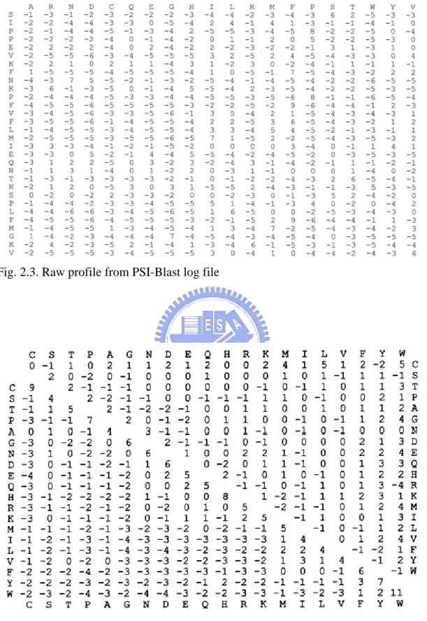
Fig. 2.3. Raw Profile From PSI-Blast Log File………...……...23
Fig. 2.4. BLOSUM 62 Matrix……….….………...23
Fig. 2.5. General Architecture of Radial Basis Function Network.…………...25
Fig. 2.6. Architecture of QuickRBF Method….…………...28
Fig. 2.7. Architecture of Two-Stage QuickRBF Method….……..……...30
Fig. 2.8. Architecture of Common Fusion QuickRBF Method…………...31
Fig. 2.9. Architecture of Local Tendency Fusion QuickRBF Method……...…...33
Fig. 2.10. Architecture of Global Tendency Fusion QuickRBF Method...…...37
Fig. 3.1. Accuracy Plot of Five Kind QuickRBF Methods...44
List of Tables
Table 2.1. Database of Non-Homologous Proteins Used For Seven-Fold Cross Validation...15
Table 2.2. Definition of Solvent Accessibility States...19
Table 2.3. Occurrence Numbers Used For Local and Global Tendency Fusion QuickRBF Methods..34
Table 3.1. Classification Accuracy of Five Kind QuickRBF Methods on The RS126 Data Set...41
Table 3.2. The accuracy tables A of Common Fusion QuickRBF on each fold and RS126...46
Table 3.3. Matthew’s Correlation Coefficients of Five Kind QuickRBF Methods on RS126...48
Chapter 1. Introduction
1.1 Motivation and The Background of This Research
The knowledge of protein structures is valuable for understanding mechanisms
of diseases of living organisms and for facilitating discovery of new drugs. Protein
structure can be experimentally determined by NMR spectroscopy and X-ray
crystallography techniques or by molecular dynamics simulations. However, the
experimental approaches are marred by long experimental time, prone to difficulties,
and expensive. There are more than 130,000 protein sequences in Swissport (release
41.20), but less than about 37,000 three-dimensional (3D) protein structure are in the
Protein Data Bank (PDB). Only a small fraction, 17%, of the enormous number of
sequenced proteins has their structure determined. In order to reduce the gap between
sequence and structure, developing reliable and applicable structure prediction
method has become a more important task in computational biology. An intermediate
but useful step is to predict protein secondary structure (PSS) or relative solvent
accessibility (RSA), which provides some knowledge and simplifies the complicated
3D structure prediction problem [1], [2]. The usual goal of RSA prediction is to
classify a pattern of residues in amino acid sequences to a pattern of solvent
accessibility elements: buried (B), intermediate (I) and exposed (E) residues. Though
the prediction of solvent accessibility is less accurate than that of secondary structure
from the homology approach, since it is less conserved than secondary structure [3],
there has been much effort to improve prediction accuracy to obtain important
tertiary structure from sequences. Many different techniques have been proposed for
RSA prediction, which broadly fall into the following categories: (1) Bayesian, (2)
neural networks, and (3) information theoretical approaches. The Bayesian methods
provide a framework to take into account local interactions among amino acid
residues, by extracting the information from single sequences or multiple sequence
alignments to obtain posterior probabilities for RSA prediction [4]. Neural networks
use residues in a local neighborhood, as inputs, to predict the RSA of a residue at a
particular location by finding an arbitrary, nonlinear mapping [5]–[8]. The
information theoretical approaches use mutual information between the sequences of
amino acids and solvent accessibility values derived from a single amino acid residue,
or pairs of residues, in a neighborhood for RSA prediction [9]. In this study, we
propose a modified QuickRBF method for RSA prediction combined with a
position-specific scoring matrix (PSSM) generated from PSI-BLAST. The QuickRBF
method, recently developed by Ou et al. [10], is applied on protein secondary
structure prediction. Our modified QuickRBF method is applied on relative solvent
accessibility prediction. We also compare the results of the modified QuickRBF
method with other methods.
1.2 Thesis Outline
The organization of this thesis is structured as follows. Chapter 1 introduces the
role of machine learning, the motivation and the background of this thesis. In Chapter
2, we will first introduce the data set and the definition of protein solvent accessibility.
Then we will propose five different kind of QuickRBF methods to predict protein
relative solvent accessibility. In Chapter 3, the experiment of computer simulation and
this thesis is presented in Chapter 4.
Chapter 2. Materials and Methods
2.1 Training and Data Set
The set of 126 nonhomologous globular protein chains used in the experiment of
Rost and Sander [3] and referred to as the RS126 set was used to evaluate the
accuracy of the prediction. The proteins in the RS126 data set have less than 25%
pairwise sequence identity. This set was used to evaluate different methods of relative
solvent accessibility prediction, for example, PHDacc [3] and other methods
[21]–[23]. In this paper, we performed a sevenfold cross-validation test on this set as
defined in Table 2.1. In order to avoid the selection of extremely biased partitions, the
RS126 set was divided into subsets of approximately same composition of each type
of RSA state. One subset was chose as the testing set while the rest was merged into
the training set. This procedure was repeated seven times to cover whole RS126 data
Table 2.1. The database of non-homologous proteins used for seven-fold cross validation. All proteins have less than 25% pairwise similarity for lengths greater than 80 residues.
256b_A 2aat 8abp 6acn 1acx 8adh 3ait
2ak3_A 2alp 9api_A 9api_B 1azu 1cyo 1bbp_A Fold_A
1bds 1bmv_1 1bmv_2 3blm 4bp2
2cab 7cat_A 1cbh 1cc5 2ccy_A 1cdh 1cdt_A
3cla 3cln 4cms 4cpa_I 6cpa 6cpp 4cpv Fold_B
1crn 1cse_I 6cts 2cyp 5cyt_R
1eca 6dfr 3ebx 5er2_E 1etu 1fc2_C 1fdl_H
1dur 1fkf 1fnd 2fxb 1fxi_A 2fox 1g6n_A Fold_C
2gbp 1a45 1gd1_O 2gls_A 2gn5
1gpl 4gr1 1hip 6hir 3hmg_A 3hmg_B 2hmz_A
5hvp_A 2i1b 3icb 7icd 1il8_A 9ins_B 1l58 Fold_D
1lap 5ldh 1gdj 2lhb 1lmb_3
2ltn_A 2ltn_B 5lyz 1mcp_L 2mev_4 2or1_L 1ovo_A
1paz 9pap 2pcy 4pfk 3pgm 2phh 1pyp Fold_E
1r09_2 2pab_A 2mhu 1mrt 1ppt
1rbp 1rhd 4rhv_1 4rhv_3 4rhv_4 3rnt 7rsa
2rsp_A 4rxn 1s01 3sdh_A 4sgb_I 1sh1 2sns Fold_F
2sod_B 2stv 2tgp_I 1tgs_I 3tim_A
1bks_A 1bks_B 1tnf_A 1ubq 2tmv_P 2tsc_A 2utg_A Fold_G
2.2 The Definition of Protein Solvent Accessibility
2.2.1 Static Residue Solvent Accessibility
The native structure of globular proteins exists only in the presence of water [11],
and therefore the analysis of their interactions with water is central to the theory of
protein structure [12]. The term “accessible surface area” was introduced by Lee and
Richards [13] to quantitatively describe the extent to which atoms on the protein
surface can form contacts with water. For a particular protein atom it is defined as the
area over which the centre of a water molecule can be placed while retaining van der
Waals contacts with that atom and not penetrating any other atom. The principal goal
is to predict the extent to which a residue embedded in a protein structure is accessible
to solvent. Solvent accessibility can be described in several ways [13]–[15]. The most
detailed fast method compiles solvent accessibility by estimating the volume of a
residue embedded in a structure that is exposed to solvent as shown in Fig. 2.1; note:
this method was developed by Lee and Richards [13] and later implemented in DSSP
[16]. Different residues have a different possible accessible area.
Studies of solvent accessibility in proteins have led to many new insights into
protein structure [13]–[18]. Knowledge of solvent accessibility has proved useful for
identifying protein function, sequence motifs, and domains, and for formulating
hypotheses about antigenic determinants, site-directed mutagenesis, humanization of
antibodies, and on the correctness of designed or experimentally determined protein
structures. Furthermore, knowledge of solvent accessibility has assisted alignments in
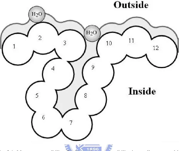
Fig. 2.1. Measure accessibility. Residue solvent accessibility is usually measured by rolling a spherical water molecule over a protein surface and summing the area that can be accessed by this molecule on each residue (typical values range from 0-300 Å2
). To allow comparisons between the accessibility of long extended and spherical amino acids, typically relative values are compiled (actual area as percentage of maximally accessible area). A more simplified description distinguishes two states: exposed (here residues numbered 1-3 and 10-12) and buried (here residues 4-9) residues. Since the packing density of native proteins resembles the crystals, values for solvent accessibility provide upper and lower limits to the number of possible inter-residue contacts.
2.2.2 Residue Relative Solvent Accessibility
How can the solvent accessibility of a residue embedded in a 3D structure be cast
into a simple number? One simple way is to count the number of water molecules in
direct contact with the residue, as estimated by the program DSSP for the first
hydration shell. For comparison between amino acids of different sizes, the relative
solvent accessibility is a useful quantity as defined in Table 2.2.
Amino acid relative solvent accessibility is the degree to which a residue in a
protein is accessible to a solvent module. The relative solvent accessibility can be
calculated by the formula as follows:
RelAcc (%) = 100 ×Acc / MaxAcc (%) ,
where Acc is the solvent accessible surface area of the residue observed in the 3D
structure, given in Angstrom units, calculated from coordinates by the dictionary of
protein secondary structure (DSSP) program [16]. The number of water molecules
around a residue can be approximated by Acc/10, and MaxAcc is the maximum value
of solvent accessible surface area of each kind of residue for a Gly-X-Gly extended
Table 2.2. Definition of solvent accessibility states.
z Solvent accessibility:
Acc = solvent accessibility of a residue (given in Å2) calculated from coordinates using DSSP [16]. W≈ Acc/10, approximates the number of water molecules around the residue.
z Relative solvent accessibility:
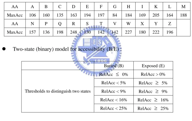
RelAcc = Acc/MaxAcc, with maximal accessibility (measured in Å2) for the amino acids given by the table following (amino acids in one-letter code; B stands for D or N; Z for E or Q, and X for an undetermined amino acid) [18][19].
AA A B C D E F G H I K L M
MaxAcc 106 160 135 163 194 197 84 184 169 205 164 188
AA N P Q R S T V W X Y Z
MaxAcc 157 136 198 248 130 142 142 227 180 222 196
z Two-state (binary) model for accessibility (B/E) :
Buried (B) Exposed (E)
RelAcc ≤ 0% RelAcc > 0% RelAcc < 5% RelAcc ≥ 5% RelAcc < 9% RelAcc ≥ 9% RelAcc < 16% RelAcc ≥ 16% Thresholds to distinguish two states
RelAcc < 25% RelAcc ≥ 25%
z Three-state (ternary) model for accessibility (B/I/E) :
Buried (B) Intermediate (I) Exposed (E) Thresholds to distinguish three states RelAcc < 9% 9% ≤ RelAcc < 36% RelAcc ≥ 36%
z Measure for evaluation of conservation and accuracy of prediction:
Q2 percentage of conserved, or correctly predicted, residues in two states defined
by thresholds given above.
Q3 percentage of conserved, or correctly predicted, residues in three states
RelAcc can hence adopt values between 0% and 100%, with 0% corresponding
to a fully buried and 100% to a fully accessible residue, respectively. Different
arbitrary threshold values of relative solvent accessibility are chose to define
categories: buried and exposed as shown in Fig. 2.2, or ternary categories: buried,
intermediate, or exposed. The precise choice of the threshold is not well defined [3].
We used two kind of class definitions: (1) buried (B) and exposed (E); and (2)
buried (B), intermediate (I), and exposed (E). For the two-state, B and E definition,
we chose various thresholds of the relative solvent accessibility such as 25%, 16%,
9%, 5%, and 0%. For the three-state, B, I, and E, description of relative solvent
accessibility, one set of thresholds that we selected is the same as those in Rost and
Sander [3]:
Buried (B): RelAcc < 9%
Intermediate (I): 9% ≤ RelAcc < 36% Exposed (E): RelAcc ≥ 36%
Fig 2.2. Binary model: thick and dark line is buried residues; thin and light line is exposed residues [20].
2.3 PSI-BLAST Profiles
It is well known that evolutionary information in the form of multiple alignments
and profiles significantly improves the accuracy of, for instance, secondary structure
prediction methods [4], [24]–[27]. This is so because the secondary structure of a
family is more conserved than the primary amino acid sequence. Similar effects have
been reported for the prediction of contact number and relative solvent accessibility.
For relative solvent accessibility, a corresponding increase of 5% has been described
both with neural networks [25] and Bayesian methods.
PSI-BLAST [28] generates the profile of a protein in the form of an N×20
position-specific scoring matrix as shown in Fig. 2.3, where N is the length of the
sequence. PSI-BLAST is run with default options, -j 3, -h 0.001, and -e 10.0, and the
non-redundant protein sequence database (ftp://ncbi.nlm.nih.gov/blast/db) filtered by
PFILT [29] to mask out regions of low complexity sequence, the coiled coil regions
and transmembrane spans. The BLOSUM62 [30] substitution matrix as shown in Fig.
2.4, is used for PSI-BLAST. These profiles were scaled to the required 0–1 range
using the standard logistic function:
) exp( 1 1 ) ( x x f − + = ,
Fig. 2.3. Raw profile from PSI-Blast log file
Fig. 2.4. BLOSUM 62 substitution matrix (Lower) and difference matrix (Upper) obtained by subtracting the PAM 160 matrix position by position. These matrices have identical relative entropies (0.70); the expected value of BLOSUM 62 is -0.52; that for PAM 160 is -0.57.
2.4 Quick Radial Basis Function Network
The radial basis function network (RBFN) is a special type of neural networks
with several distinctive features [31]. Since its first proposal, the RBFN has attracted
a high degree of interest in research communities. A RBFN consists of three layers,
namely the input layer, the hidden layer, and the output layer. The input layer
broadcasts the coordinates of the input vector to each of the nodes in the hidden layer.
Each node in the hidden layer then produces an activation based on the associated
radial basis function. Finally, each node in the output layer computes a linear
combination of the activations of the hidden nodes. How a RBFN reacts to a given
input stimulus is completely determined by the activation functions associated with
the hidden nodes and the weights associated with the links between the hidden layer
and the output layer. The general mathematical form of the output nodes in a RBFN is
as follows: cj(x) =
∑
= k i 1 wjiΦ( ||x-μi ||;σi ) ,where cj(x) is the function corresponding to the j-th output unit (class-j) and is a linear
combination of k radial basis functions Φ(.) with centerμi and bandwidthσi . Also, wj
is the weight vector of class-j and wji is the weight corresponding to the j-th class and
i-th center. The general architecture of RBFN is shown in Fig. 2.5. It can be seen that
constructing a RBFN involves determining the number of centers, k, the center
locations, μi , the bandwidth of each center, σi , and the weights, wji. That is, training a
RBFN involves determining the values of three sets of parameters: the centers (μi ),
the bandwidths (σi ), and the weights (wji), in order to minimize a suitable cost
Fig. 2.5. General architecture of Radial Basis Function Network
In QuickRBF package [10], it is focused on the calculation of the weights, and
conducting a simple method to determine the centers and bandwidths. Therefore, it
selects the centers randomly in the package. Also, it utilizes a fixed bandwidth of each
kernel function, which is set to five for each kernel function. After the centers and
bandwidths of the kernel functions in the hidden layer have been determined, the
transformation between the inputs and the corresponding outputs of the hidden units is
now fixed. The network can thus be viewed as an equivalent single-layer network
with linear output units. Then, the Least Mean Square Error method is used to
determine the weights associated with the links between the hidden layer and the
output layer.
Ou used a single-layer Quick Radial Basis Function Network [10] to analyze
protein secondary structure with excellent prediction results on the RS126 data set.
There are more details about QuickRBF can be found in QuickRBF package
(http://csie.org/~yien/quickrbf/index.php). Here, we propose a modified QuickRBF
2.5 Coding Scheme
As with Hua and Sun’s work [32], the present analysis used the classical local
coding scheme of the protein sequences with a sliding window. PSI-BLAST matrix
with n rows and 20 columns can be defined for single sequence with n residues. For
the first layer in the prediction, each residue is represented using 20 components in a
vector, based on the PSSM. In order to allow a window to extend over the N-terminus
and the C-terminus, an additional 21st unit (spacer) was attached to each residue.
Then, each input vector has 21×w components, where w is a sliding window size. For
the second layer, the vector corresponding to a residue has four elements in the
three-state prediction and three elements in the two-state prediction, where the first
three elements represent the three relative solvent accessibility states, E, I, and B, in
the three-state prediction and the first two elements represent the two relative solvent
accessibility states, E and B, in the two-state prediction. Both the last units were
added in order to allow a window to extend over the N-terminus and the C-terminus.
If the window length is v, the dimension of the feature vector is 4×v for the second
2.6 Several Prediction System Structures
Five different kind of QuickRBF approaches are applied on three-state, E, I, and
B, and two-state, E and B, relative solvent accessibility predictions. These five
approaches include: (1) QuickRBF, (2) Two-Stage QuickRBF, (3) Common Fusion
QuickRBF, (4) Local Tendency Fusion QuickRBF, and (5) Global Tendency Fusion
QuickRBF.
2.6.1 QuickRBF Approach
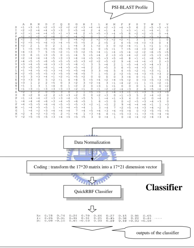
A QuickRBF structure was used in the prediction system as shown in Fig. 2.6.
The QuickRBF classifier classifies each residue of each sequence into the three
relative solvent accessibility states, E, I, or B, by using the values of matrices of
PSI-BLAST profile as the inputs. The outputs represent the tendency that the residue
belongs to that state. The one-against-rest strategy was used for the multiclass
classification, so each residue was classified into the state with the largest output
Fig. 2.6. Architecture of QuickRBF method. The system includes two parts: the PSI-BLAST profile, and the classifier. The profile is transformed into a number of 21*17 dimension vectors using the slide-window method. These vectors are input into the QuickRBF classifier. The outputs of the QuickRBF classifier are a number of 3D vectors representing the tendency that the residue belongs to that state. The one-against-rest strategy was used to classify each residue into the state with the largest value.
PSI-BLAST Profile
Coding : transform the 17*20 matrix into a 17*21 dimension vector
QuickRBF Classifier Data Normalization
Classifier
2.6.2 Two-Stage QuickRBF Approach
A Two-Stage QuickRBF structure was used in the prediction system as shown in
Fig. 2.7. The first stage is a QuickRBF classifier that classifies each residue of each
sequence into the three relative solvent accessibility states, E, I, or B, by using the
values of matrices of PSI-BLAST profile as the inputs. The outputs of the first stage
represent the tendency that the residue belongs to that state. The second stage
QuickRBF classifier also classifies each residue of each sequence into the three
relative solvent accessibility states, E, I, or B, by using the RSA three-state tendency
matrices from the outputs of the first stage as the inputs. The outputs of the second
stage also represent the tendency that the residue belongs to that state. As with an
One-Stage QuickRBF approach, the second stage also uses the one-against-rest
strategy, with each residue classified into the state with the largest output value for a
Second Stage
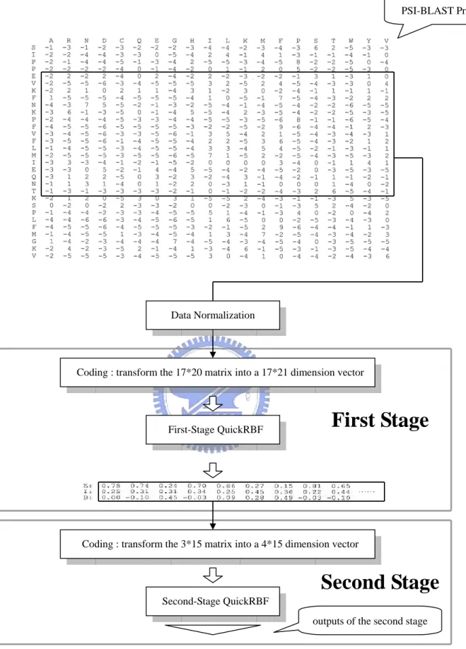
Fig. 2.7. Architecture of Two-Stage QuickRBF method. The system includes three parts: the PSI-BLAST profile, the first stage, and the second stage. The profile is transformed into a number of 21*17 dimension vectors using the slide-window method. These vectors are input into the first-stage QuickRBF. The outputs of the first-stage QuickRBF are a number of 3D vectors representing the tendency that the residue belongs to that state. Using the slide-window method, the outputs of the first-stage QuickRBF are transformed into a number of 4*15 dimensional vector, which are used as the inputs of the second-stage QuickRBF. The final decisions are based on the outputs of the second-stage QuickRBF.
PSI-BLAST Profile
Coding : transform the 17*20 matrix into a 17*21 dimension vector
First-Stage QuickRBF Data Normalization
Coding : transform the 3*15 matrix into a 4*15 dimension vector
Second-Stage QuickRBF
First Stage
2.6.3 Common Fusion QuickRBF Approach
Three kind of fusion QuickRBF approaches were used to combine the outputs of
a QuickRBF approach and the outputs of a Two-Stage QuickRBF approach. One is
the Common Fusion QuickRBF approach, and the others are the Local Tendency
Fusion QuickRBF approach and the Global Tendency Fusion QuickRBF approach.
The architectures of these three approaches were illustrated in Figs. 2.8, 2.9, and 2.10.
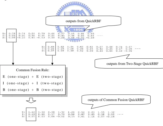
The common fusion strategy adds up the tendency outputs from a QuickRBF
approach and the tendency outputs from a Two-Stage QuickRBF approach. Then we
also use the one-against-rest strategy to classify each residue into the state with the
largest value.
Fig. 2.8. Architecture of Common Fusion QuickRBF method
Common Fusion Rule:
E ( o n e - s t a g e ) + E ( t w o - s t a g e ) I ( o n e - s t a g e ) + I ( t w o - s t a g e ) B ( o n e - s t a g e ) + B ( t w o - s t a g e )
outputs from QuickRBF
outputs from Two-Stage QuickRBF
2.6.4 Local Tendency Fusion QuickRBF Approach
The local tendency fusion strategy also adds up the tendency outputs from a
QuickRBF approach and the tendency outputs from a Two-Stage QuickRBF approach.
An occurrence number table is then applied in the summation as shown in Table 2.3.
There are three occurrence numbers which are Oe, Oi and Ob, where Oe means the
numbers of exposed components in the test data, and Oi means the numbers of
intermediate components in the test data, and Ob means the numbers of buried
components in the test data. These three occurrence numbers represent the potential
factors for the affection ability of the three relative solvent accessibility states. In
other words, if an occurrence number is larger, the tendency of a residue which
belongs to that state is larger. Then we also use the one-against-rest strategy to
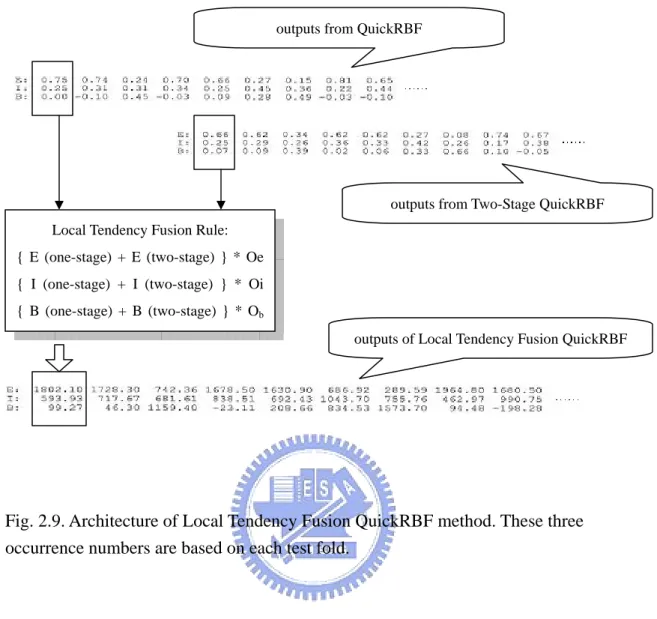
Fig. 2.9. Architecture of Local Tendency Fusion QuickRBF method. These three occurrence numbers are based on each test fold.
outputs from QuickRBF
Local Tendency Fusion Rule: { E (one-stage) + E (two-stage) } * Oe { I (one-stage) + I (two-stage) } * Oi { B (one-stage) + B (two-stage) } * Ob
outputs from Two-Stage QuickRBF
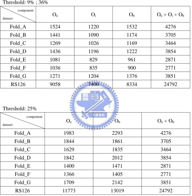
Table 2.3. Occurrence numbers used for local and Global Tendency Fusion QuickRBF method. From Fold_A to Fold_G, these occurrence numbers of each fold are used for Local Tendency Fusion QuickRBF method. And the occurrence numbers of RS126 dataset are used for Global Tendency Fusion QuickRBF method.
Threshold: 9% ; 36% Threshold: 25% component dataset Oe Ob Oe + Ob Fold_A 1983 2293 4276 Fold_B 1844 1861 3705 Fold_C 1629 1835 3464 Fold_D 1842 2012 3854 Fold_E 1400 1471 2871 Fold_F 1366 1405 2771 Fold_G 1709 2142 3851 RS126 11773 13019 24792 component dataset Oe Oi Ob Oe + Oi + Ob Fold_A 1524 1220 1532 4276 Fold_B 1441 1090 1174 3705 Fold_C 1269 1026 1169 3464 Fold_D 1436 1196 1222 3854 Fold_E 1081 829 961 2871 Fold_F 1036 835 900 2771 Fold_G 1271 1204 1376 3851 RS126 9058 7400 8334 24792
Table 2.3.(continued) Threshold: 16% component dataset Oe Ob Oe + Ob Fold_A 2373 1903 4276 Fold_B 2231 1474 3705 Fold_C 1977 1487 3464 Fold_D 2261 1593 3854 Fold_E 1679 1192 2871 Fold_F 1630 1141 2771 Fold_G 2083 1768 3851 RS126 14234 10558 24792 Threshold: 9% component dataset Oe Ob Oe + Ob Fold_A 2744 1532 4276 Fold_B 2531 1174 3705 Fold_C 2295 1169 3464 Fold_D 2632 1222 3854 Fold_E 1910 961 2871 Fold_F 1871 900 2771 Fold_G 2475 1376 3851 RS126 16458 8334 24792
Table 2.3.(continued) Threshold: 5% component dataset Oe Ob Oe + Ob Fold_A 3028 1248 4276 Fold_B 2769 936 3705 Fold_C 2502 962 3464 Fold_D 2866 988 3854 Fold_E 2098 773 2871 Fold_F 2048 723 2771 Fold_G 2773 1078 3851 RS126 18084 6708 24792 Threshold: 0% component dataset Oe Ob Oe + Ob Fold_A 3652 624 4276 Fold_B 3297 408 3705 Fold_C 3010 454 3464 Fold_D 3378 476 3854 Fold_E 2536 335 2871 Fold_F 2451 320 2771 Fold_G 3360 491 3851 RS126 21684 3108 24792
2.6.5 Global Tendency Fusion QuickRBF Approach
The global tendency fusion strategy is mostly the same with the local tendency
fusion strategy. The difference between these two tendency fusion strategies is that
these three occurrence numbers used for the global tendency fusion strategy are the
occurrence numbers of three kind of components in the RS126 data set.
Fig. 2.10. Architecture of Global Tendency Fusion QuickRBF method. These three occurrence numbers are based on the RS126 data set.
outputs from QuickRBF
Global Tendency Fusion Rule: { E (one-stage) + E (two-stage) } * Oe { I (one-stage) + I (two-stage) } * Oi { B (one-stage) + B (two-stage) } * Ob
outputs from Two-Stage QuickRBF
Chapter 3. Experiment and Simulation Results
3.1 Experiment Procedure of Five QuickRBF Approaches
Five different kind of QuickRBF approaches are applied on three-state, E, I, and
B, and two-state, E and B, relative solvent accessibility predictions. These five
methods are QuickRBF, Two-Stage QuickRBF, Common Fusion QuickRBF, Local
Tendency Fusion QuickRBF, and Global Tendency Fusion QuickRBF.
For QuickRBF, One-Stage QuickRBF approach, each residue is coded as a
21-dimensional vector, where the first 20 elements of the vector are the corresponding
elements in PSI-BLAST matrix and the last unit was added in order to allow a
window to extend over the N- and the C-terminus. The window length is 17 and the
dimension of the feature vector is 21×17. The number of the centers randomly
selected from the training data set is 12000 and the bandwidth is five for each kernel
function. The architecture of QuickRBF in the three-state prediction is shown
previously in Fig. 2.6.
For Two-Stage QuickRBF, the window lengths are 17 for the first layer and 15
for the second layer. The dimension of the feature vector for the first layer is 21×17.
The dimensions of the feature vectors for the second layer are 4×15 in the three-state
prediction and 3×15 in the two-state prediction. The numbers of the centers randomly
selected from the training data set are 12000 for the first layer and 500 for the second
layer. The bandwidths are both five for the first and second layer. The architecture of
These three kind of fusion strategies, Common Fusion, Local Tendency Fusion,
and Global Tendency Fusion, are the combinations of One-Stage QuickRBF and
Two-Stage QuickRBF. Different rules are used for each fusion strategy. The
architectures of these three fusion strategies in the three-state prediction are shown
previously in Figs. 2.8, 2.9, and 2.10.
3.2 Classification Accuracy of Five QuickRBF Approaches
The results and the comparison of the five different kind of QuickRBF
approaches on RS126 data set are listed in Table 3.1. On the RS126 data set,
QuickRBF gave the overall prediction accuracy 59.67% for the three-state prediction
with respect to thresholds: 9%; 36% and 87.99%, 80.06%, 78.46%, 76.98%, 75.60%,
respectively for the two-state prediction with respect to thresholds of 0%, 5%, 9%,
16%, 25%.
Two-Stage QuickRBF gave the overall prediction accuracy 59.11% for the
three-state prediction with respect to thresholds: 9%; 36% and 87.55%, 79.25%,
78.21%, 76.15%, 73.76%, respectively for the two-state prediction with respect to
thresholds of 0%, 5%, 9%, 16%, 25%.
Common Fusion QuickRBF gave the overall prediction accuracy 60.07% for the
three-state prediction with respect to thresholds: 9%; 36% and 87.82%, 80.15%,
78.58%, 77.13%, 75.66%, respectively for the two-state prediction with respect to
Local Tendency Fusion QuickRBF gave the overall prediction accuracy 59.91%
for the three-state prediction with respect to thresholds: 9%; 36% and 87.60%,
77.20%, 75.84%, 76.54%, 75.55%, respectively for the two-state prediction with
respect to thresholds of 0%, 5%, 9%, 16%, 25%.
Global Tendency Fusion QuickRBF gave the overall prediction accuracy 59.91%
for the three-state prediction with respect to thresholds: 9%; 36% and 87.60%,
77.25%, 75.82%, 76.43%, 75.48%, respectively for the two-state prediction with
respect to thresholds of 0%, 5%, 9%, 16%, 25%.
The accuracy plot of the above the five kind QuickRBF approaches is shown in
Fig. 3.1 and Common Fusion QuickRBF is numbered three. Among these five
QuickRBF approaches, Common Fusion QuickRBF has better performance for either
the three-state prediction or the two-state prediction. Common Fusion QuickRBF is
then decided as our modified QuickRBF approach because of the better performance
Table 3.1. RSA classification accuracy of five kind QuickRBF methods on the RS126 data set with PSI-BLAST pssm profiles.
QuickRBF accuracy: % threshold dataset 3-state (9% ; 36%) 2-state (0%) 2-state (5%) 2-state (9%) 2-state (16%) 2-state (25%) Fold_A 61.25 86.72 80.52 78.70 78.16 76.92 Fold_B 60.11 88.77 81.30 79.65 77.84 76.06 Fold_C 62.99 87.90 81.76 81.18 79.19 77.77 Fold_D 59.37 88.53 80.95 79.09 77.09 75.61 Fold_E 60.85 88.65 81.92 80.22 78.65 76.63 Fold_F 59.11 89.03 81.60 79.18 76.18 74.27 Fold_G 53.99 86.32 72.34 71.18 71.75 71.90 Average 59.67 87.99 80.06 78.46 76.98 75.60 Two-Stage QuickRBF accuracy: % threshold dataset 3-state (9% ; 36%) 2-state (0%) 2-state (5%) 2-state (9%) 2-state (16%) 2-state (25%) Fold_A 60.71 86.62 80.43 78.30 76.52 74.58 Fold_B 60.59 88.18 78.11 78.79 76.73 75.17 Fold_C 62.73 88.14 81.41 81.21 77.34 77.74 Fold_D 57.16 88.30 79.94 78.15 75.71 72.00 Fold_E 59.80 88.92 81.85 80.49 77.81 72.34 Fold_F 58.72 88.92 80.04 77.55 75.78 72.21 Fold_G 54.06 83.80 72.97 72.97 73.18 72.29 Average 59.11 87.55 79.25 78.21 76.15 73.76
Table 3.1. (continued)
Common Fusion QuickRBF
accuracy: % threshold dataset 3-state (9% ; 36%) 2-state (0%) 2-state (5%) 2-state (9%) 2-state (16%) 2-state (25%) Fold_A 61.20 86.67 80.40 78.53 77.95 76.19 Fold_B 61.27 88.88 80.59 79.54 78.19 76.90 Fold_C 63.40 88.08 81.67 81.67 78.96 78.09 Fold_D 59.06 88.43 80.83 78.54 76.93 74.73 Fold_E 61.20 88.75 82.41 80.74 78.34 76.04 Fold_F 59.33 88.70 81.81 78.85 76.69 74.92 Fold_G 55.05 85.23 73.36 72.16 72.84 72.76 Average 60.07 87.82 80.15 78.58 77.13 75.66
Local Tendency Fusion QuickRBF
of accuracy: % threshold dataset 3-state (9% ; 36%) 2-state (0%) 2-state (5%) 2-state (9%) 2-state (16%) 2-state (25%) Fold_A 60.69 85.45 76.38 75.89 75.96 76.31 Fold_B 60.89 88.99 79.00 77.11 77.30 76.87 Fold_C 62.96 87.01 78.41 78.03 79.27 78.38 Fold_D 59.70 87.68 78.20 76.99 77.19 74.18 Fold_E 60.92 88.30 78.44 77.01 77.85 75.62 Fold_F 59.18 88.49 78.20 77.05 76.15 74.77 Fold_G 55.03 87.25 71.80 68.79 72.06 72.73 Average 59.91 87.60 77.20 75.84 76.54 75.55
Table 3.1. (continued)
Global Tendency Fusion QuickRBF
accuracy: % threshold dataset 3-state (9% ; 36%) 2-state (0%) 2-state (5%) 2-state (9%) 2-state (16%) 2-state (25%) Fold_A 60.29 85.48 76.08 75.07 75.16 76.61 Fold_B 61.16 89.02 79.16 77.38 77.92 76.65 Fold_C 63.05 87.01 78.32 78.06 79.30 78.32 Fold_D 59.68 87.68 78.41 77.43 77.30 74.16 Fold_E 60.89 88.26 78.44 77.05 78.23 75.44 Fold_F 59.26 88.49 78.49 77.27 76.18 74.67 Fold_G 55.05 87.25 71.88 68.50 70.89 72.50 Average 59.91 87.60 77.25 75.82 76.43 75.48
Comparison of five kind QuickRBF methods
accuracy: % threshold method 3-state (9% ; 36%) 2-state (0%) 2-state (5%) 2-state (9%) 2-state (16%) 2-state (25%) QuickRBF 59.67 87.99 80.06 78.46 76.98 75.60 Two-Stage QuickRBF 59.11 87.55 79.25 78.21 76.15 73.76
Common Fusion QuickRBF 60.07 87.82 80.15 78.58 77.13 75.66
Local Tendency Fusion QuickRBF 59.91 87.60 77.20 75.84 76.54 75.55
50 55 60 65 70 75 80 85 90 9& 36 0 5 9 16 25 T hreshold (%) Ac cu ra cy ( % )
1: QuickRBF
2: Two-Stage QuickRBF
3: Common Fusion QuickRBF
4: Local Tendency Fusion QuickRBF
5: Global Tendency Fusion QuickRBF
3.3 Matthew’s Correlation Coefficients of Five QuickRBF Approaches
Another measure used to evaluate the performance of prediction methods is the
Matthew’s Correlation Coefficient (MCC). It can be calculated from an accuracy table
A by the following equations:
ij
A = number of residues predicted to be in type j and observed to be in type i,
) )( )( )( ( i i i i i i i i i i i i i o n u n o p u p o u n p MCC + + + + − = , i p = A , ii i n =
∑∑
≠ ≠ 3 3 i j k i jk A , i o =∑
≠ 3 i j ji A , i u =∑
≠ 3 i j ij A , for i = E, I, B.Also, pi , ni , oi and ui are the number of true positives, true negatives, false positives
and false negatives for class i, respectively. The MCCs have the same value for the
two classes in the case of the two-state prediction, i.e. MCCE = MCCB.
First, the accuracy tables A of Common Fusion QuickRBF on each fold and the
RS126 data set is shown in Table 3.2. Then, the MCCs of five kind QuickRBF
methods on the RS126 data set is shown in Table 3.3. In a similar trend as Table 3.1,
MCC’s of Common Fusion QuickRBF usually perform well, although not always the
Table 3.2. The accuracy tables A of Common Fusion QuickRBF on each fold and RS126. 3-state (9%; 36%) AEE AII ABB AEI AEB AIE AIB ABE ABI Fold_A 1276 294 1042 141 107 587 339 277 213 Fold_B 1134 285 837 187 120 455 350 144 193 Fold_C 1033 257 905 130 106 433 336 138 126 Fold_D 1067 276 940 180 189 433 487 145 137 Fold_E 843 196 724 132 106 347 286 120 117 Fold_F 816 170 645 113 107 387 278 155 100 Fold_G 835 279 1011 207 229 434 491 174 191 RS126 7004 1757 6104 1090 964 3076 2567 1153 1077 2-state (25%) AEE ABB AEB ABE Fold_A 1695 1563 288 730 Fold_B 1417 1432 427 429 Fold_C 1247 1458 382 377 Fold_D 1244 1636 598 376 Fold_E 952 1231 448 240 Fold_F 996 1080 370 325 Fold_G 1109 1693 600 449 RS126 8660 10093 3113 2926 2-state (16%) AEE ABB AEB ABE Fold_A 2134 1199 239 704 Fold_B 1842 1055 389 419 Fold_C 1613 1122 364 365 Fold_D 1803 1162 458 431 Fold_E 1402 847 277 345 Fold_F 1368 757 262 384 Fold_G 1596 1209 487 559 RS126 11758 7351 2476 3207
Table 3.2. (continued) 2-state (9%) AEE ABB AEB ABE Fold_A 2489 869 255 663 Fold_B 2228 719 303 455 Fold_C 2051 778 244 391 Fold_D 2300 727 332 495 Fold_E 1742 576 168 385 Fold_F 1657 528 214 372 Fold_G 2003 776 472 600 RS126 14470 4973 1988 3361 2-state (5%) AEE ABB AEB ABE Fold_A 2818 620 210 628 Fold_B 2449 537 320 399 Fold_C 2259 570 243 392 Fold_D 2660 455 206 533 Fold_E 1939 427 159 346 Fold_F 1885 382 163 341 Fold_G 2245 580 528 498 RS126 16255 3571 1829 3137 2-state (0%) AEE ABB AEB ABE Fold_A 3612 94 40 530 Fold_B 3206 87 91 321 Fold_C 2956 95 54 359 Fold_D 3330 78 48 398 Fold_E 2473 75 63 260 Fold_F 2416 42 35 278 Fold_G 3202 80 158 411 RS126 21195 551 489 2557
Table 3.3. Matthew’s Correlation Coefficients of Five Kind QuickRBF Methods on RS126. 3-state (9%; 36%) MCC method MCCE MCCI MCCB QuickRBF 0.477 0.146 0.500 Two-Stage QuickRBF 0.485 0.130 0.491
Common Fusion QuickRBF 0.488 0.142 0.502
Local Tendency Fusion QuickRBF 0.487 0.123 0.508 Global Tendency Fusion QuickRBF 0.489 0.123 0.505
2-state (25%) MCC
method MCCE = MCCB
QuickRBF 0.517
Two-Stage QuickRBF 0.476
Common Fusion QuickRBF 0.511
Local Tendency Fusion QuickRBF 0.439
Global Tendency Fusion QuickRBF 0.440
2-state (16%) MCC
method MCCE = MCCB
QuickRBF 0.524
Two-Stage QuickRBF 0.512
Common Fusion QuickRBF 0.528
Local Tendency Fusion QuickRBF 0.514
Table 3.3. (continued) 2-state (9%) MCC method MCCE = MCCB QuickRBF 0.493 Two-Stage QuickRBF 0.499
Common Fusion QuickRBF 0.500
Local Tendency Fusion QuickRBF 0.513
Global Tendency Fusion QuickRBF 0.513
2-state (5%) MCC
method MCCE = MCCB
QuickRBF 0.449
Two-Stage QuickRBF 0.457
Common Fusion QuickRBF 0.464
Local Tendency Fusion QuickRBF 0.482
Global Tendency Fusion QuickRBF 0.483
2-state (0%) MCC
method MCCE = MCCB
QuickRBF 0.249
Two-Stage QuickRBF 0.262
Common Fusion QuickRBF 0.256
Local Tendency Fusion QuickRBF 0.281
3.4 Comparison with other Approaches
Comparison of performance of modified QuickRBF approach with other
methods in RSA prediction on the RS126 data set is shown in Table 3.4. Accuracy
plot of modified QuickRBF approach and other methods is shown in Fig. 3.2.
Modified QuickRBF, Common Fusion, is our method, and reported 60.1% for
the three-state prediction with respect to 9%; 36% thresholds, and 87.8%, 80.2%,
78.6%, 77.1%, 75.7%, respectively for the two-state predictions with respect to
thresholds of 0%, 5%, 9%, 16%, 25%.
Fuzzy k-NN (Sim, Kim and Lee, 2005) used fuzzy k-nearest neighbor method
[23] using PSI-BLAST profiles as feature vectors, and shows slightly better prediction
accuracies than other methods on the RS126 data set ,and reported 63.8% for the
three-state prediction with respect to 9%; 36% thresholds, and 87.2%, 82.2%, 79.0%,
78.3%, respectively for the two-state predictions with respect to thresholds of 0%, 5%,
16%, 25%.
PHDacc (Rost and Sander, 1994) used a neural network method [3] using
evolutionary profiles of amino acid substitutions derived from multiple sequence
alignments, and reported 57.5% for the three-state prediction with respect to 9%; 36%
thresholds, and 86.0%, 74.6%, 75.0%, respectively for the two-state predictions with
SVMpsi (Kim and Park, 2004) was based on a support vector machine [21] using
the position-specific scoring matrix generated from PSI-BLAST, and reported 59.6%
accuracy for the three-state prediction with respect to 9%; 36% thresholds and 86.2%,
79.8%, 77.8%, 76.8%, respectively accuracies for the two-state predictions with
respect to thresholds of 0%, 5%, 16%, 25%.
Two-Stage SVMpsi (Nguyen and Rajapakse, 2005) used a Two-Stage SVMpsi
approach [22] using the position-specific scoring matrix generated from PSI-BLAST,
and reported 90.2%, 83.5%, 81.3%, 79.4%, respectively accuracies for the two-state
predictions with respect to thresholds of 0%, 5%, 9%, 16%. These prediction
accuracies are obtained from their published results. The three state accuracy of
Modified QuickRBF is 60.1%, which is 3.7% lower than Fuzzy k-NN (63.8%) and
Table 3.4. Comparison of performance of modified QuickRBF approach with other methods in RSA prediction on the RS126 data set with PSSMs generated by PSI-BLAST.
PHDacc (Rost and Sander, 1994) used neural networks [3].
SVMpsi (Kim and Park, 2004) was based on support vector machine [21].
Two-Stage SVMpsi (Nguyen and Rajapakse, 2005) used a two-stage SVM approach [22]. Fuzzy k-NN (Sim, Kim and Lee, 2005) used fuzzy k-nearest neighbor method [23].
accuracy: % threshold method 3-state (9%; 36%) 2-state (0%) 2-state (5%) 2-state (9%) 2-state (16%) 2-state (25%)
Modified QuickRBF (Common Fusion) 60.1 87.8 80.2 78.6 77.1 75.7
PHDacc 57.5 86.0 ─ 74.6 75.0 ─
SVMpsi 59.6 86.2 79.8 ─ 77.8 76.8
Two-Stage SVMpsi ─ 90.2 83.5 81.3 79.4 ─
50 55 60 65 70 75 80 85 90 95 9& 36 0 5 9 16 25 Threshold (%) A ccu racy ( % )
1: Modified QuickRBF (Common Fusion)
2: PHDacc
3: SVMpsi
4: Two-stage SVMpsi
5: Fuzzy k-NN
Chapter 4.
Conclusion and Discussion
In this study, we have applied the five QuickRBF approaches, which are
QuickRBF, Two-Stage QuickRBF, Common Fusion QuickRBF, Local Tendency
Fusion QuickRBF, and Global Tendency Fusion QuickRBF, to predict relative solvent
accessibility, using PSI-BLAST profiles as feature vectors. Our best method,
Common Fusion QuickRBF, achieved the similar performance as the researches did in
the recent years. Because the goal of this thesis was to provide a new approach for
relative solvent accessibility, the results suggest that the modified QuickRBF
approach is a successful one.
In the future strategy, we can apply our method on a larger data set. Data set
growth can give an indirect advantage to our method. And our modified QuickRBF
References
[1] J. Chandonia and M. Karplus, “New methods for accurate prediction of protein
secondary structure,” Protein Engineering, vol. 35, pp. 293–306, 1999.
[2] D.W. Mount, “Bioinformatics: sequence and genome analysis,” Cold Spring
Harbor, NY: Cold Spring Harbor Laboratory Press, 2001.
[3] B. Rost and C. Sander, “Conservation and prediction of solvent accessibility in
protein families,” Proteins, vol. 20, pp. 216–226, 1994.
[4] M.J. Thompson and R.A. Goldstein, “Predicting solvent accessibility: higher
accuracy using Bayesian statistics and optimized residue substitution classes,”
Proteins, vol. 47, pp. 142–153, 1996.
[5] S. Pascarella, R.D. Persio, F. Bossa, and P. Argos, “Easy method to predict
solvent accessibility from multiple protein sequence alignments,” Proteins, vol.
32, pp. 190–199, 1999.
[6] X. Li and X.M. Pan, “New method for accurate prediction of solvent
accessibility from protein sequence,” Proteins, vol. 42, pp. 1–5, 2001.
[7] G. Pollastri, P. Baldi, P. Fariselli, and R. Casadio, “Prediction of coordination
number and relative solvent accessibility in proteins,” Proteins, vol. 47, pp.
142–153, 2002.
[8] S. Ahmad and M.M. Gromiha, “NETASA: neural network based prediction of
solvent accessibility,” Bioinformatics, vol. 18, pp. 819–824, 2002.
[9] H. Naderi-Manesh, M. Sadeghi, S. Araf, and A.A.M. Movahedi, “Predicting of
protein surface accessibility with information theory,” Proteins, vol. 42, pp.
[10] Y.Y. Ou, “QuickRBF is an Efficient Construction of Radial Basis Function
Networks with the Cholesky Decomposition,” http://csie.org/~yien/quickrbf/ .
[11] J.D. Bernal, I. Fankuchen, and M. Perutz, “An X-Ray study of chymotrypsin and
haemoglobin,” Nature, vol. 141, pp. 523–524, 1938.
[12] W.A. Kauzmann, “Some factors in the interpretation of protein denaturation,”
Protein Chem., vol. 14, pp. l–63, 1959.
[13] B.K. Lee and F.M. Richards, “The interpretation of protein structures: estimation
of static accessibility,” J. Mol. Biol., vol. 55, pp. 379–400, 1971.
[14] C. Chothia, “The nature of the accessible and buried surfaces in proteins,” J. Mol.
Biol., vol. 105, pp. 1–12, 1976.
[15] M.L. Connolly, “Solvent-accessible surfaces of proteins and nucleic acids,”
Science, vol. 221, pp. 709–713, 1983.
[16] W. Kabsch and C. Sander, “Dictionary of protein secondary structure: pattern
recognition of hydrogen-bonded and geometrical features,” Biopolymers, vol. 22,
pp. 2577–2637, 1983.
[17] J. Janin, “Surface and inside volumes in globular proteins,” Nature, vol. 277, pp.
491–492, 1979.
[18] G.D. Rose, A.R. Geselowitz, G.J. Lesser, R.H. Lee, and M.H. Zehfus,
“Hydrophobicity of amino acid residues in globular proteins,” Science, vol. 229,
pp. 834–838, 1985.
[19] C. Sander, M. Scharf, and R. Schneider, “Design of protein structures in: Protein
Engineering: A practical Approach,” Oxford University press, pp. 89–115, 1992
[20] H. Hirakawa and S. Kuhara, “Prediction of Hydrophobic Cores of Proteins Using
Wavelet Analysis,” Genome Inform Ser Workshop Genome Information, vol. 8,
[21] H. Kim and H. Park, “Prediction of protein relative solvent accessibility with
support vector machines,” Proteins, vol. 54, pp. 557–562, 2004.
[22] M.N. Nguyen and J.C. Rajapakse, “Prediction of protein relative solvent
accessibility with a two-stage SVM approach,” Proteins, vol. 59, pp. 30–37,
2005.
[23] J. Sim, S.Y. Kim, and J. Lee, “Prediction of protein solvent accessibility using
fuzzy k-nearest neighbor method,” Bioinformatics, vol. 21, pp. 2844–2849, 2005.
[24] D.T. Jones, “Protein secondary structure prediction based on position specific
scoring matrices,” J. Mol. Biol., vol. 292, pp. 195–202, 1999.
[25] B. Rost and C. Sander, “Combining evolutionary information and neural
networks to predict protein secondary structure,” Proteins, vol. 19, pp. 55–72,
1994.
[26] G.J. Barton, “Protein secondary structure prediction,” Curr. Opin. Struct. Biol.,
vol. 5, pp. 372–376, 1995.
[27] P. Baldi, S. Brunak, P. Frasconi, G. Pollastri, and G. Soda, “Exploiting the past
and the future in protein secondary structure prediction,” Bioinformatics, vol. 15,
pp. 937–946, 1999.
[28] S.F. Altschul et al., “Gapped BLAST and PSI-BLAST: a new generation of
protein database search programs,” Nucleic Acids Res., vol. 25, pp. 3389–3402,
1997.
[29] D.T. Jones, “Protein secondary structure prediction based on position-specific
scoring matrices,” J. Mol. Biol., vol. 292, pp. 195–202, 1999.
[30] S. Henikoff and J.G. Henikoff, “Amino acid substitution matrices from protein
blocks,” Proc. Natl. Acad. Sci., vol. 89, pp. 10915–10919, 1992.
[32] S. Hua and Z. Sun, “A novel method of protein secondary structure prediction
with high segment overlap measure: support vector machine approach,” J. Mol.
![Fig 2.2. Binary model: thick and dark line is buried residues; thin and light line is exposed residues [20]](https://thumb-ap.123doks.com/thumbv2/9libinfo/8451714.182547/21.892.160.731.112.600/binary-model-thick-buried-residues-light-exposed-residues.webp)