最適匯率目標區理論與實證-以臺灣為例 - 政大學術集成

全文

(1)國立政治大學經濟學系 National Chengchi University Department of Economics. 碩士論文 Master’s Thesis. 政治大. 指導教授: 毛維凌教授. 學最適匯率目標區理論與實證 –以臺灣為例. Nat. y. ‧. ‧ 國. 立. sit. n. al. er. io. Optimal Policy Rule with Target Zone: Theory and Application to Taiwan. Ch. engchi. 研究生: 李宇峻 Yu-Chun Li 2010 年 7 月. i n U. v.

(2) 謝辭時光匆匆, 短短兩年的研究生生涯就這樣結束了。過程中需要感謝的人太多, 雖然如此, 不能夠只謝天, 必定要好好的感謝一路上給予我幫助的人。首先要感謝的是李慧琳老師, 在尚未開學的時候, 幫助我讓我能夠有宿舍, 不用煩惱在外租屋會遇到的種種問題。再來是資源教室的黃老師, 兩年內提供給我的工讀機會, 對我的生活開銷有相當. 政治大教授毛維凌老師, 謝謝你給我很多的啟發以及彈性 , 在我迷路的時候立. 大的幫助。還要感謝的當然是在我的論文中最重要的角色, 我的指導. ‧ 國. 學. 指引我回到正確的道路。也希望老師能夠好好的保重身體, 一直都健康、開心。當然也要感謝兩位口試委員, 朱美麗老師和方振瑞老師, 謝. ‧. 謝朱美麗老師給的建議, 非常受用; 方振瑞老師, 那時知道校外口試. y. Nat. 委員是您的時候, 真是又驚又喜, 驚是因為巧合, 喜是因為這一切馬. n. a. er. io. 論文的提點, 真的是針針見血, 鞭辟入理!. sit. 上變得很熟悉, 就像當初在上您的課一樣。感謝方振瑞老師對於我的. v. l C 研究所生涯中結識了許多同學 , 大家對我的幫忙都不少 , 但是有幾 ni. hengchi U. 位在此要特別提出來。第一位是我們盡心盡力盡責的班代靖翰, 謝謝你這麼貼心的給我最需要的幫助, 欠你的一頓我絕對不會忘記。第二位是魏祥庭, 雖然只是一小步, 但你的熱心卻成就了我整篇論文, 謝謝你。還有郭晏伶, 出唱片的理想, 我等妳!還有很多很多的同學, 在這裡我都要致上我最誠摯的謝意, 謝謝你們。最後, 感謝閱讀這篇論文的您, 能完成這篇論文, 政大豐富的資源功不可沒!.

(3) 摘要這篇論文主要探討的是現任央行總裁彭淮南上任後, 央行對於匯率管理上的政策行為。我們觀察從 1999 年到 2009 年這段期間的名目有效匯率發現, 雖然匯率波動於一個區間之內, 但名目有效匯率在大部份的期間都是被低估的, 尤其是近幾年來更是相當的偏低。所以我們懷疑臺灣央行所管制的匯率目標區他們較希望能維. 政治大. 持新臺幣在被低估的水準, 當新臺幣匯率受到高估時, 央行則希望能將其下修。為. 立. 了探討這個情況, 我們透過 Krugman(1991) 所發表的匯率目標區模型來試著得. ‧ 國. 學. 到新臺幣的最適匯率行為。又因為臺灣的特殊經濟背景, 我們融合了 Chen,Funke 和 Glanemann(2009) 的寬鬆邊界匯率目標區模型和 Torres(2000) 的隨機邊界內. ‧. 的央行干預模式來修正傳統的 Krugman 模型。然而, 傳統的 Krugman 模型我. y. Nat. er. io. sit. 們得到最重要的結論是, 當匯率越接近上下邊界時會有越強烈的蜜月效果, 也就是說匯率的波動越平緩。但是當我們融入上面兩種修正在配合新臺幣的名目有效匯. al. n. v i n Ch 率實際資料時, 我們發現蜜月效果僅僅存在於下界 U e n g c h i , 就算是央行所保護的區間有變動時, 在下界還是相對於上界穩定相當多。這就是因為在下界存在著強烈的蜜月效果, 所以匯率在越接近下界時會越穩定, 甚至有很大機率維持在下界附近。這個結論跟我們觀察實際資料所發現的現象是相當符合的, 所以能夠解釋為什麼新臺幣的名目有效匯率會總是被低估。.

(4) Abstract. This paper discusses the policy rule used by Central Bank of the Republic of China(Taiwan) with target zone to the exchange rate dynamics. We focus on the recent phenomena on the exchange rate of NTD, and try to figure why the NEER of NTD is always underestimated. Due to the regime of. 政治大. Central Bank of the Republic of China(Taiwan), we combine two extensions. 立. into the basic Krugman(1991) target zone model which are Chen, Funke. ‧ 國. 學. and Glanemann’s soft edge target zone model(2009) and Torres’s stochastic intra-marginal intervention pattern. And we estimate the parameters with. ‧. simulated method of moments(SMM). By this two extensions, we conclude. y. Nat. er. io. sit. that there is strong honeymoon effect to the exchange rates at the lower bound, but the honeymoon effect is very weak at the upper bound. This. al. n. v i n conclusion is matched with C thehempirical data, and e n g c h i U explains why the NEER of NTD is always underestimated..

(5) Contents 1 Introduction. 1. 2 Literature Review. 3. 2.1. Lack of Credibility . . . . . . . . . . . . . . . . . . . . . . . .. 4. 2.2. Intra-Marginal Interventions . . . . . . . . . . . . . . . . . . .. 6. 2.3. Summary . . . . . . . . . . . . . . . . . . . . . . . . . . . . . 11. 立. 3 Model. 政治大. 13. ‧ 國. 學. Soft Edge Target Zone Model . . . . . . . . . . . . . . . . . . 15. 3.2. Stochastic Intra-marginal Intervention . . . . . . . . . . . . . 17. ‧. 3.1. y. Nat. io. sit. 4 Econometric Methodology. 19. Empirical Application . . . . . . . . . . . . . . . . . . . . . . 19. 4.2. Simulated Method of Moments(SMM) . . . . . . . . . . . . . 21. n. al. er. 4.1. Ch. engchi. i n U. 5 Empirical Results. v. 25. 5.1. Data . . . . . . . . . . . . . . . . . . . . . . . . . . . . . . . . 25. 5.2. Estimation . . . . . . . . . . . . . . . . . . . . . . . . . . . . . 26. 6 Conclusion. 33. A The Continuous-time Monetary Model. 35.

(6) B Derivation of Equation(10) and (11). 37. C Brownian motion, Wiener process, random walk. 37. D Stochastic Calculus. 38. E Solution of Krugman’s Model. 41. F SAS Code. 立. Reference. 政治大. 44. 46. ‧. ‧ 國. 學. n. er. io. sit. y. Nat. al. Ch. engchi. 6. i n U. v.

(7) 1. Introduction Taiwan is a small-open economy whose economic development depends. greatly on export. In the 1970s, due to the continuously enlarging gap of favorable balance of trade to the U.S., the new Taiwan dollar(NTD) was forced to appreciate. Therefore, the central bank of Taiwan switched from the fixed exchange rate regime to a managed float regime in July 1978.. 治政 Thereafter, the central bank of Taiwan aims 大 at reducing the fluctuation 立 ‧ 國. 學. of the exchange rates, i.e. leaning against the wind, so that the economy will involve in less speculative risks. When the foreign exchange market, for. ‧. instance, faces a capital inflow shock, the domestic money must appreciate. Nat. sit. y. to accommodate the excess demand. But appreciation will have impact both. n. al. er. io. on the domestic exporter as well as the GDP. So the central bank must. i n U. v. intervene to defend the domestic currency so that the NTD will depreciate.. Ch. engchi. On the other hand, if the exchange rate keeps depreciating, the domestic currency then becomes weaker and demand of our currency will give us a lot of pressure to appreciate. As described above, we presume that the exchange rates are likely to fluctuate in an existing band despite that it is not claimed by the central bank. And this is referred to a target zone issue of the European Monetary. 1.

(8) System(EMS) during the 1980s. Krugman (1991) presents a plausible and tractable target zone model which is a standard framework of many works for the target zone analysis. These works point out that Krugman model does not fit the empirical data, and presume that this failure may result in two corruption of the basic assumptions: perfect credibility and marginal intervention.. 政治大. Chen,Funke and Glanemann (2009) illustrate a problem of lacking cred-. 立. ibility in a soft edge target zone model with an application to Hong Kong’s. ‧ 國. 學. currency board arrangement. Torres (2000) introduces a stochastic intra-. grates both efforts in order to fit empirical data better.. Nat. sit. y. ‧. marginal intervention into the standard target zone model. Our work inte-. io. er. The organization of this paper is as the following, we review the litera-. al. tures in section 2. Section 3 sets up the soft edge target zone model with. n. v i n Ch U description of econometstochastic intra-marginal intervention. e n gThen c hai brief. ric methodology we propose for estimation is presented in section 4. Section 5 shows the empirical results and section 6 concludes.. 2.

(9) 2. Literature Review. The seminal paper of Krugman (1991) was the first explicitly to analyze the effects if exchange rate bounds on exchange rate behavior. The basic two assumptions of his model are full credibility and marginal intervention which contribute to dampen the expected change of exchange rate while the exchange rates are heading toward the bounds. This dampening is so-called ”honeymoon effect”.. 治政大 of exchange rates is Moreover, the long-run density 立. ‧ 國. 學. U-shaped, i.e. with a large concentration of probability mass close to the boundaries. (see Svensson 1991a). ‧. However, as a modeling vehicle for the EMS, there is a strong evidence. Nat. sit. y. that it fails to account for a number of stylized facts, of which the most. n. al. er. io. important is the evidence on the empirical distributions of most EMS ex-. i n U. v. change rate in their bands. In practice, these unconditional distributions. Ch. engchi. tend to be hump-shaped, with most of the probability mass concentrated inside the band. For example, Bertola and Caballero (1992) present empirical evidence about the hump-shaped feature of the distribution of the French franc against the Deutsche Mark(the Ffr/DM rate) for the period April 1979 through December 1987. They offer an explanation based on repeated realignments of the exchange rate band and also provide an empirical evidence. 3.

(10) on interest rate differentials, which at times indicates expectations of future realignments. Using non-parametric methods on a variety if exchange rate, interest rate and fundamental data, Meese and Rose (1990) and Flood, Rose and Mathieson (1991) do not find any evidence if significant non-linearities : the components left unexplained by non-linear models are highly serial correlated and , in many cases, so large as to raise serious doubts on the. 政治大. empirical validity of target-zone models. Thus, new models often referred to. 立. the second-generation models extend the Krugman model in two alternative. ‧ 國. 學. directions: lack of credibility and/or intra-marginal interventions.. Lack of Credibility. ‧. 2.1. Nat. sit. y. Bertola and Caballero (1992) allow for exogenous realignment risk in the. n. al. er. io. target zone model. The monetary authorities will defend the currency with. i n U. v. probability (1-p) when it reaches the edges of the band and will proceed with. Ch. engchi. realignment of the central parity with probability (p). The model with exogenous realignment risk implies that under certain circumstances (p ≥ 0.5) , both the honeymoon effect and smooth pasting will disappear. In such a high realignment probabilities, the relationship between exchange rates and fundamentals becomes inverted-S shaped because large exchange-rate volatility is expected by the market participants. They expect that the currency will. 4.

(11) not be defended so that the exchange rate is volatile when it heads toward the band. Clearly, the fact that realignment is modeled as exogenous and realignment only takes places when the exchange rate is at the edge of the band may be too restrictive and need not apply in reality. Tristani (1994) and Werner (1995) set out to model realignment risk as endogenous by assuming. 政治大. that the probability of realignment is a positive function of how far the ex-. 立. change rate is located from central parity. That is, the larger is the distance,. ‧ 國. 學. the higher is the probability of realignment. This in turn implies an even. ‧. stronger U-shaped distribution of the exchange rate within the band. Bertola and Svensson (1993) incorporate stochastic devaluation risk in. sit. y. Nat. io. er. target zone model in order to discuss the time-vary realignment risk. Many. al. empirical data reveal that the monetary authorities in Europe realign not. n. v i n C h zone, but inside only at the edges of the target e n g c h i U the band for stabilizing the exchange rates. Hence, the realignment risk is defined as an exogenous and stochastic process which varies across time. However, the relationship between exchange rate and interest rate differential becomes uncertain in their model. This uncertainty explains that, in real world, the exchange rate and interest rate differential need not to be a tradeoff. But the distribution of exchange rates within the band is still U-shaped ,which does not fit the 5.

(12) empirical data. Recently, the adoption of common currency makes target zone analysis less applicable for European issues. However, the analysis is still relevant for developing and newly industrialized countries in Latin America and Asia that occasionally fix their exchange rate to the dollar. Chen, Funke and glanemann (2009) discuss the Hong Kong’s currency board arrangement policy by. 政治大. a soft band target zone model. They assume that the announced edges ,s and. 立. s, are normally distributed. The variance of the band variable reflects the. ‧ 國. 學. degree of confidence market participants have in the band given the econ-. ‧. omy’s current and expected fundamentals. The resulting dynamics of the exchange rate are again S-shaped which is monotonically increasing function. sit. y. Nat. io. er. of the degree of confidence market participants have in the band given the. al. economy’s current and expected fundamentals. The soft edge target zone. n. v i n C h hard band curveU as the exchange rate apcurves become steeper than the engchi. proaches the edges. Therefore, soft edge band leads to weaker honeymoon effect and wider target zone range.. 2.2. Intra-Marginal Interventions. Mastropasqua et al. (1988) and Delgado and Dumas(1992) argue that about 85 to 90 percent of total interventions took the form of intra-marginal in-. 6.

(13) tervention in the ERM before the crises in 1992 and 1993. Regarding the post-crisis periods , the exchange rate never hit the upper of lower bound of any of the participating countries, which implies that all interventions were necessarily intra-marginal. As a result, it comes as no surprise that the distribution of the exchange rate is usually found to be hump-shaped for currencies participating in ERM and ERM-2, suggesting that the exchange. 政治大. rate spends most of the time in the middle of the band rather than close to. 立. the boundaries of the target zone.. ‧ 國. 學. Delgado and Dumas (1992) modify the Krugman model so as to account. ‧. for intra-marginal interventions assumed to take place continuously inside the target zone if the exchange rate deviates from the central parity. Although. sit. y. Nat. io. er. the honeymoon effect diminishes considerably when compared to counter-. al. part under perfect credibility and marginal intervention, the exchange rate. n. v i n C is nonetheless less volatile thanhunder Similarly, smooth pasting is e n gfree-float. chi U also substantially reduced in this set-up because market agents know that the monetary authorities have already intervened. These interventions induce a mean reversion of the exchange rate towards the central parity. Even in the absence of a formal target-zone-type of exchange rate arrangement, central bank interventions can stabilize the exchange rate better than the case of a free-float. 7.

(14) A major drawback of the models presented above is that they are based, without exception, on the flexible-price monetary model, which assumes that purchasing power parity(PPP) holds steadily. However, it is a wellestablished fact that PPP does not hold steadily, and therefore some kind of rigidities should be introduced into the modeling framework. Following the example of the Dornbusch overshooting model, Miller and Weller(1991). 政治大. introduce sticky prices into the Krugman model. In addition to sticky prices,. 立. Beetsma and Ploeg(1994) complete the model with intra-marginal interven-. ‧ 國. 學. tions and show that sticky prices coupled with intra-marginal interventions. zone.. ‧. leads to a hump-shaped distribution of the exchange rate within the target. sit. y. Nat. io. er. Torres (2000) applies the technique of Bertola and Svensson’s (1993). al. stochastic devaluation risk to a stochastic intra-marginal intervention pro-. n. v i n C supply changes areU(negative) proportional to cess. He assumes that money h engchi the velocity shocks, and such a policy is referred to a ”leaning against wind” policy. This implies the existence of continuous change in money supply will offset changes in velocity shocks in order to preserve the band of fluctuation.. As a result, this kind of intra-marginal interventions cause a reduction of the bandwidth of the fundamentals. As interventions increase, the honeymoon effect disappears. On the other hand, the intra-marginal interventions imply 8.

(15) a reduction of both instantaneous standard deviation of the exchange rate and interest rate differential. Hence, there is no trade-off between exchange rate and interest rate variability. These results can explain the empirical failure in testing for non-linearities in exchange rate and interest rate differentials in current target zones. Bessec (2003) proposes that it is unlikely that the monetary authorities. 政治大. would be willing to intervene continuously, independently of the distance of. 立. the exchange rate from the central parity. Instead, she argues that it is more. ‧ 國. 學. likely that monetary authorities do not intervene in the immediate neigh-. ‧. borhood of the central parity and allow the exchange rate to fluctuate in a given corridor around the central parity. Only if the exchange rate exits. sit. y. Nat. io. er. this corridor do the monetary authorities step in to intervene. This kind. al. of regime can be described by the combination of the Krugman model and. n. v i n C h uses the self-exciting Delgado-Dumas model. And she e n g c h i U threshold autoregressive(SETAR) model as econometric specification. Although the theoretical. model suggests that it is only intra-marginal interventions by the monetary authorities that create a band of inaction, it is worth nothing that, in practice, a large number of other factors may also be accounted for. He includes the ability of the monetary authorities to stabilize the national currency by other policy action. Second, moral persuasion and appropriate communica9.

(16) tion towards the markets are also likely to influence the exchange rate. More particularly, market expectations and the credibility of monetary authorities are likely to play a key role. If the monetary authorities are credible, it may suffice to intervene in very small amounts in the market to persuade agents that the exchange rate will remain stable. Or, even better, the possibility of market intervention and a well-established tracking record of the monetary. 政治大. authorities may bring about relative exchange rate stability.. 立. Finally, expectations may also be stabilized because of fundamentals be-. ‧ 國. 學. coming increasingly stable, or because of expected future developments of the. ‧. fundamentals. This kind of effect may have played a special role in the runup to the euro in the late 1990s, when the markets expected a high degree of. sit. y. Nat. io. er. macroeconomic convergence to occur across countries. Therefore, the band. al. of inaction could be viewed as a band where the exchange rate dynamics. n. v i n C h whereas outsideUthe band, the above factors resemble a random walk process engchi can result in the exchange rate mean reverting. Crespo-Cuaresma, Egert and MacDonald (2005) suggest that the above factors is best captured by a three-regime SETAR model conditional variance by means of a GARCH(1,1).. 10.

(17) 2.3. Summary. Although Krugman’s standard target zone model presents an easy way to discuss the target zone issue, its performance is bad on fitting the empirical data. This is resulted from the strength of honeymoon effect which is overemphasized. After that, the extensions of imperfect credibility and intra-marginal intervention both try to reduce the strength of honeymoon. 政治大. effect so as smooth pasting. In this paper, we integrate the combination. 立. of Chen, Funke and Glanemann’s(2009) framework(lack of credibility) with. ‧ 國. 學. Torres’s (2000) device(stochastic intra-marginal intervention) and apply to. ‧. the analysis for Taiwan’s case.. sit. y. Nat. Why choose these two set-ups? The soft edge target zone model which. n. al. er. io. applies to Hong Kong whose has so much in common with Taiwan. For ex-. i n U. v. ample, Hong Kong’s currency board was established in 1983 and the Hong. Ch. engchi. Kong dollar(HKD) was pegged to the US dollar(USD) at 7.8 to 1. In September 1998, the exchange rate changed to 7.75 to 1. The exchange rate moved gradually from 7.75 back to 7.80 between 1999 and August 2000. Since late 2003, speculative pressure for a revaluation of the Chinese Renminbi has grown, with the result of large speculative inflows. The HKD appreciated from 7.80 to 7.70 in autumn 2003, fueling speculation that the currency board link to the USD might be abandoned. The currency board arrange11.

(18) ment was again altered on 18 May 2005 when finally a narrow symmetric target zone of ±0.6 percent was introduced with a strong-side Convertibility Undertaking. 1. at HKD 7.75/USD. For the first time, this added a ceiling. to the floor by which it had traditionally managed the currency, in a move to discourage investors from using HKD 7.8/USD to HKD7.85/USD. Parallelly, new Taiwan dollar(NTD) was pegged to the USD at 40 to 1 before. 政治大. 1986. Later, with huge accumulation of foreign reserve, NTD is forced to. 立. appreciate. The central bank of Taiwan changed the fixed exchange rate. ‧ 國. 學. to managed float regime. The NTD appreciated from NTD 39.59/USD to. ‧. NTD 28.101/USD from January 1986 through December 1987. Nevertheless, it seems no currency board decision for the central bank of Taiwan rule. sit. y. Nat. io. er. in coping with speculation. Presumably, the central bank takes stochastic. al. intra-marginal interventions when facing stochastic speculative shocks. The. n. v i n C perceived issue from above arehmodeled section of this paper. There i U e n g inc hnext are two subsections which the first one is the soft edge target zone model and the second one is adding stochastic intra-marginal intervention to the model. 1. Since bank notes issued are backed up by an equivalent amount of foreign currencies (US dollars since 1983), our currency system is one with a foreign exchange standard. It is known as the Linked Exchange Rate System. The arrangement (minor amendment in 2006 due to the effect of an appreciation of Renminbi) allows note issuing banks, (now extended to all licensed banks) to buy and sell HK dollars and U.S. dollars with the Exchange Fund at a fixed exchange rate. (about 1 USD to 7.8 HKD depends whether HKD is on the strong side or on the weak side. The convertibility undertaking is within 500 points around 7.8 HKD. That is between 7.75 HKD and 7.85 HKD). However, the exchange market is still ”free” to trade Hong Kong dollar currency as well as other currencies with floating exchange rates.. 12.

(19) 3. Model. Let us first briefly review the basic Krugman (1991) framework with perfectly known and credible bands to gain a benchmark for future analysis. The model starts from the log-linear asset pricing equation that expresses the log exchange rate, s, as the sum of the log of fundamentals, f, and its own expected change s=f+. α E[ds] dt. 立. 政治大. (1). ‧ 國. 學. where f = m + v and m is assumed to be zero, E[•] denotes the rational expectations operator, α > 0, and time subscripts are omitted for brevity. The. ‧. factors affecting the exchange rate are fundamentals and financial markets’. Nat. sit. y. expectations about the future movement of the exchange rate. It is assumed. n. al. er. io. that the log of fundamentals follows an arithmetic Brownian motion with drift: df = µdt + σdW. Ch. engchi. i n U. v. (2). where µdt is the expected change in f conditional on information available at t, σ is the risk parameter and W denotes a standard Brownian motion.. 2. Applying Itˆ o’s lemma to the expectations term yields3 : s = f + αµ ds + df 2 3. ασ 2 d2 s 2 f2. (3). It is also referred to a Wiener process or random walk. See Appendix D. 13.

(20) Krugman (1991) specified the dynamics of f between two limits4 The lower and upper band limits, s and s, result from the intervention obligations within the target zone arrangement. This gives rise to a reflected of regulated Brownian motion. The particular solution of equation (1) is as sp = f + αµ, showing the unregulated exchange rate dynamics. The homogeneous solution, sH representing the changes in value from the intervention of the. 政治大. central bank is. 立. where β1 = − σµ2 +. q. µ2 σ4. +. (4). 2 , ασ 2. β2 = − σµ2 −. q. µ2 σ4. 2 ασ 2. +. 學. ‧ 國. sH = −A1 eβ1 f + A2 eβ2 f. and A1 and A2 are posi-. ‧. tive coefficients. The exponential terms A1 eβf and A2 e−βF cause the bending of the exchange rate function and thus generate the target zone nonlinear-. sit. y. Nat. io. al. n. we obtain the S-shaped exchange rate function. Ch. engchi. s = f + αµ + A1 eβ1 f + A2 eβ2 f. er. ities. Expressing the exchange rate as an explicit function of fundamentals. i n U. v. (5). which is the general solution of the form for the exchange rates. The band edges come from two value-matching conditions. s = f + αµ + A1 eβ1 f + A2 eβ2 f. (6). s = f + αµ + A1 eβ1 f + A2 eβ2 f. (7). where s and s are strong and weaker band exchange rates and f and f are 4. See Appendix E. 14.

(21) the levels of fundamentals as the edges of the bands are approached. The noexpected-arbitrage-profits conditions imply the following two smooth-pasting conditions, which require that the exchange rate function is flat at the edges 0 = 1 + A1 β1 eβ1 f + A2 β2 eβ2 f. (8). 0 = 1 + A1 β1 eβf + A2 β2 eβ2 f. (9). Equation (6) (9) enable determination of the two constants of integration,. 政治大. A1 and A2 , which completely solve the model. β1 [e. β2 [e. (β1 f +β2 f ). β1 f. e. 立. β2 f. −e. (β1 f +β2 f ) ]. −eβ1 f −e. (β1 f +β2 f ) ]. <0. (10). 學. A2 =. eβ2 f −e (β1 f +β2 f ). ‧ 國. A1 =. >0. (11). ‧. After obtaining f , f , A1 and A2 , a S-shaped curve can be obtained through equation (5).. sit. y. Nat. Soft Edge Target Zone Model. io. n. al. er. 3.1. i n U. v. In the original Krugman (1991) model, the reduced form relationship be-. Ch. engchi. tween exchange rates and fundamentals is driven by the perfectly known and credible bands. Conversely, what happens when the relationship is driven not by the band itself but by expectations regarding the band? To keep the model tractable, the soft edge band is assumed to consist of two components: the announced edges s and s, and a normal distributed noise term. In normal times, the noise term is small. But in noisy times, when confidence is. 15.

(22) fragile, capital inflows may cause a crisis of confidence that sets off massive capital flows. In other words, we replaced the perfectly Known and credible symmetric band [s, s] by [N (s, σs2 ), N (s, σs2 )] and we analyze how the uncertainty as to the band feeds back into the dynamics of the exchange rate. The variance σs2 reflects the degree of confidence market participants have in the band given the economy’s current and expected fundamentals.. 政治大. To keep the exchange rate within the symmetric band [N (s, σs2 ), N (s, σs2 )],. 立. it is sufficient to confine the fundamental process to [N (f , σs2 ), N (f , σs2 )] at. ‧ 國. 學. both ends. By taking expectations conditional on the information of f , f. ‧. and σs2 , we obtain the following perceived value-matching conditions for the soft model, as shown in the Appendix B:. n. 2 β1 σs ) 2. Ch. + A2 eβ2 (f +. 2 β2 σs ) 2. engchi U. E[s|s, σs2 ] = E[f + αµ + A1 eβ1 f + A2 eβ2 f |f , σs2 ] → s = f + αµ + A1 eβ1 (f +. 2 β1 σs ) 2. + A2 eβ2 (f +. 2 β2 σs ) 2. er. io. al. → s = f + αµ + A1 eβ1 (f +. sit. y. Nat. E[s|s, σs2 ] = E[f + αµ + A1 eβ1 f + A2 eβ2 f |f , σs2 ]. v ni. (12). (13). The corresponding smooth-pasting conditions are 0 = 1 + A1 β1 eβ1 (f + 0 = 1 + A1 β1 eβ1 (f +. 2 β1 σs ) 2 2 β1 σs ) 2. + A2 β2 eβ2 (f + + A2 β2 eβ2 (f +. 2 β2 σs ) 2. (14). 2 β2 σs ) 2. (15). Equation (12) (15) enable determination of the two constants of integration, t t Asof and Asof , which completely solve the model. 1 2. 16.

(23) β1 [e. 2 β σ2 β2 σs β (f + 22 s ) 2 ) −e 2 β σ2 β σ2 β σ2 β σ2 β1 (f + 12 s )+β2 (f + 22 s ) β1 (f + 12 s )+β2 (f + 22 s ). −e. ]. β1 [e. 2 β σ2 β1 σs β1 (f + 12 s ) −eβ1 (f + 2 ) β σ2 β σ2 β σ2 β σ2 β1 (f + 12 s )+β2 (f + 22 s ) β1 (f + 12 s )+β2 (f + 22 s ). ]. eβ2 (f +. t = Asof 1 t Asof 2. 3.2. e. =. −e. <0. (16). >0. (17). Stochastic Intra-marginal Intervention. Torres (2000) introduces a target zone model with stochastic intra-marginal intervention. Again, the exchange rate dynamics are given by. 政治大. t] t] = ft + α E[ds st = mt + vt + α E[ds dt dt. 立. The fundamentals is a composite of the velocity shocks, vt , and the money. ‧ 國. 學. supply,mt . So the change of fundamentals is. ‧. dft = dvt + dmt. sit. y. Nat. where dvt = µv dt + σv dWv,t. io. al. er. In the standard target zone model, changes in money supply occur only at. v. n. the edge of the band. However, we assume that money supply follows a. Ch. engchi. Brownian motion process inside the band.. i n U. dmt = µm dt + σm dWm,t if ht 6= 0, otherwise dmt = 0 where ht is the deviation of the fundamentals from its central parity. Allowing for possible correlation ρ between its increments, we can drive the velocity shocks process, dWv,t dWm,t = ρdt, |ρ| ≤ 1 So the new fundamental process is 17.

(24) dft = µf dt + σf dWf,t where µf = µv + µm , σf =. q. 2 + 2ρσ σ σv2 + σm v m. The intervention rule is that the central bank intervenes by changing the money supply in a manner opposite to the velocity shocks changes, because it is in its interest to maintain the aggregate fundamentals closing to their central value. So we may assume that dmt = −γdvt. 立. 政治大. where 0 < γ < 1 is the monetary intervention parameter. The greater. ‧ 國. 學. the monetary intervention parameter, the greater the likelihood of similarity. ‧. between both processes. If γ = 0, we have the marginal intervention case. If γ = 1, we are in a perfect fixed exchange rate system. After illustrating the. sit. y. Nat. io. al. er. intervention rule of the central bank, the fundamental process evolves into. n. µf = (1 − γ)µv , σf = (1 − γ)σv Apply Itˆ o’s lemma. Ch. engchi. i n U. v. st = ft + α(1 − γ)µv s0 (ft ) + α2 [σv (1 − γ)]2 s00 (ft ) and the general solution for st is st = ft + α(1 − γ)µv + A1 eβ1 ft + A2 eβ2 ft √ √ 2 2 [(1−γ)σv ]2 (1−γ)µv − [(1−γ)µv ]2 + α [(1−γ)σv ]2 (1−γ)µv + [(1−γ)µv ]2 + α i i where β1 = − , β = − 2 2 2 [(1−γ)σv ] [(1−γ)σv ]. 18.

(25) 4. Econometric Methodology. 4.1. Empirical Application. DeJong(1994) estimates the Krugman model by maximum likelihood and by simulated method of moments(SMM) using weekly data from January 1987 to September1990. He ends his sample in 1990 so that exchange rate affected by news or expectations about German reunification, which culminated in. 政治大. the European Monetary System crisis of September 1992, are not included.. 立. We will follow DeJong’s SMM estimation strategy to estimate the basic. ‧ 國. 學. Krugman model.. 5. ‧. ∆ft = µ + σ ε˜t. sit. y. Nat. st = αµ + ft + A1 eβ1 ft + A2 eβ2 ft. iid. β2 =. − σµ2. −. q. µ2 σ4. q. µ2 σ4. +. al. 2 ασ 2. >0. +. 2 ασ 2. <0. n. β1 = − σµ2 +. er. io. where f = −f , the time unit is one day(∆t = 1), and ε˜t ∼ N (0, 1).. Ch. engchi. i n U. v. and A1 = A2 =. eβ2 f −e β1 [e. (β1 f +β2 f ). β2 [e. (β1 f +β2 f ). β1 f. e. β2 f. −e. (β1 f +β2 f ) ]. −eβ1 f −e. (β1 f +β2 f ) ]. <0 >0. Log exchange rates are normalized by their central parities and multiplied by 100. The parameters to be estimated are (µ, α, σ, f , f ). SMM is covered 5. See Appendix D. 19.

(26) in next subsection. Denote the simulated observations with a ”star(*)”. You need to simulate sequences of the fundamentals that are guaranteed to stay within the ˆ = f ∗ + µ + σ ε˜i bands[f , f ]. You can do this by letting fi+1 i     ˆ − f∗   2f − fi+1 i     . ∗ ˆ =  fi+1 fı+1 . , if. ˆ ≥f fi+1. , if. ˆ ≥f f ≥ fi+1. 政治 , if 大f ˆ.       ˆ − f∗   2f − fi+1 i. 立. 6. and setting. ≤f. i+1. (18)7. ‧ 國. 學. for ı = 1, · · · , M . The simulated exchange rates are given by ∗. ∗. ‧. s∗ı (µ, α, σ, f , f ) = fı∗ + αµ + A1 eβ1 fı + A2 eβ2 fı ,. y. . n. al. Ch. 1 M. ∆s∗i. 1 M. PM. ∆s∗i 2. i=3. i=3. e n g c Ph i 1 M. M i=3. er. io.           ∗ HM [s (µ, α, σ, f , f )] =          . . PM. sit. Nat. the simulated moments are by. i n U. v. ∆s∗i 3. 1 M. PM. ∆s∗i ∆s∗i−1. 1 M. PM. ∆s∗i ∆s∗i−2. i=3. i=3.                    . (19) The sample moments are based on the first three moments and the first two 6. In practice, the available data observations are discrete. Let us approximate the continuous time model(the diffusion process) by a model with a discrete but arbitrary small time unit ∆ = n1 (Euler approximation). 7 It will generate no observations exactly on the bounds. Otherwise, such observations cause problems.. 20.

(27) autocovariances. The first two moments are the expectation and the variance, because these are likely to be sensitive to the drift parameter, µ, and the variance parameter, σ 2 , of the fundamental process. In addition, we use the third moments (skewness) and the first and the second autocovariances of the exchange rate. These moments are included to capture the non-linear part of the exchange rate process.. 政治 ∆s 大. . . ∆s2t. 1 T. PT. ∆s3t. 1 T. PT. ∆st ∆st−1. 1 T. PT. ∆st ∆st−2. t=3. t=3. t=3. y. t=3.                    . n. al. (20). er. io. 4.2. PT. t. sit. Nat with M=20T.. 1 T. t=3. ‧. ‧ 國. 立. 1 T. 學.           HT (s) =          . PT. i n U. C. v. h eofn Moments(SMM) Simulated Method gchi. Consider a collection of empirical targets contained in the r ∗ 1 vector h(zt ), where zt denotes an T ∗ 1 vector variables observed at time t. Let yt denote an T ∗ 1 vector of model variables that correspond directly to their empirical counterparts zt , and h(yt , θ),where θ is a q ∗ 1 vector of parameters, denote the theoretical counterparts to h(zt ). Under GMM, E[h(yt , θ)] is calculated analytically; under SMM this need not be the case. Instead, all that is 21.

(28) required is the ability to simulate yt using a parameterization of the structural model under investigation. Proceeding under the usual assumption that the model has been specified for stationary versions of the data, the sample average h(Υ, θ) =. 1 N. PN. i=1. h(yt , θ),. 0 0 0 where Υ = [yN , yN −1 , ·, y1 ]. (4.2.1). 政治大. is an asymptotically consistent estimator of E[h(yt , θ)]. the idea behind SMM. 立. estimators is to use sample averages in place of population averages in eval-. ‧ 國. 學. uating implications of the structural model regarding h(yt , θ).. sit. y. Nat. eterization of the structural model θ0 under which. ‧. SMM estimator proceeds under the hypothesis that there exists a param-. (4.2.2). io. er. Eh(zt ) = Eh(yt , θ). the objective is to choose parameter estimates θˆ that come as close as possible. n. al. to satisfying this equity.. v i n C h of notation used In terms e n g c h i U in discussing the GMM. estimator, f (zt , θ0 ) is given by f (zt , θ0 ) = h(zt ) − h(yt , θ0 ). (4.2.3). and the sample analogue g(Z, θ) is given by g(Z, θ) = HT (s) − HM [s∗ (η, α, σ, f , f )] where HT (s) and HM [s∗ (η, α, σ, f , f )] are given in equation (15) and (16).. 22.

(29) The optimal weighting matrix8 Ω∗ is given by the inverse of the variancecovariance matrix Σ associated with the sample mean of g(Z, θ). Under the null hypothesis (4.2.2), the sample means of h(zt ) and h(yt , θ) are identical. Moreover, the empirical and artificial samples zt and yt are independent. Thus because g(Z, θ) is a linear combination of independent sample means, its variance-covariance matrix is given by. 政治大. Σ(1 + T /N ). 立. Note that as the artificial sample size N increases relative to T, the covariance. ‧ 國. 學. matrix of g(Z, θ) converges to its GMM counterpart. This is true because as. ‧. N increases, the influence of the numerical error associated with the use of a. sit. y. Nat. sample average to approximate E[h(yt , θ)] decreases.. io. al. n. Ω∗ = Σ(1 + T /N ). er. With the adjustment. Ch. engchi U. v ni. (4.2.4). estimation and testing via GMM and SMM proceed identically. To briefly summarized, the objective function used to estimate θˆ is given by argmin Γ(θ) θ. = g(Z, θ)0 [Σ((1 + T )/N )]−1 g(Z, θ). where Σ is given by either Σ=. 1 T. PT. t=1. f (zt , θ)f (zt , θ)0. or 8. See Nelson, Structural Macroeconometrics p.154. 23. (4.2.5).

(30) Σ = Γ0 + Γv =. 1 T. Ps. v=1 (1. PT. t=v+1. +. v )(Γv s+1. + Γ0v ). f (zt , θ)f (zt−v , θ)0. The circular relationship between θ and Σ necessitates an iterative estimation procedure under which an initial estimate θˆ0 is obtained using an identity ˆ 0 and the process is repeated until the matrix for Σ, θˆ0 is used to construct Σ ˆ converge. estimates θˆ and Σ. 政治大. ˆ is given Under mild regularity conditions, the limiting distribution of Σ. 立. 學. √. ‧ 國. by. T (θˆ − θ0 ) → N (0, V ). ‧. where V = (DΣD0 )−1 and D’ is a q*r gradient matrix. y. sit. io. al. er. ∂g(Z,θ) ∂θ0. Nat. D0 =. n. ˆ denoting the evaluation of D obtained using Σ, ˆ V is estimated using With D ˆΣ ˆ −1 D ˆ 0 )−1 Vˆ = (D. Ch. engchi. i n U. v. Finally, the null hypothesis can be evaluated using a modification of Hensen’s(1982) J statistic: √ √ ˆ 0 [Σ(1 ˆ ˆ + T /N )]−1 [ T g(Z, θ)] J = [ T g(Z, θ)] which is distributed asymptotically as χ2 (r − q). 24.

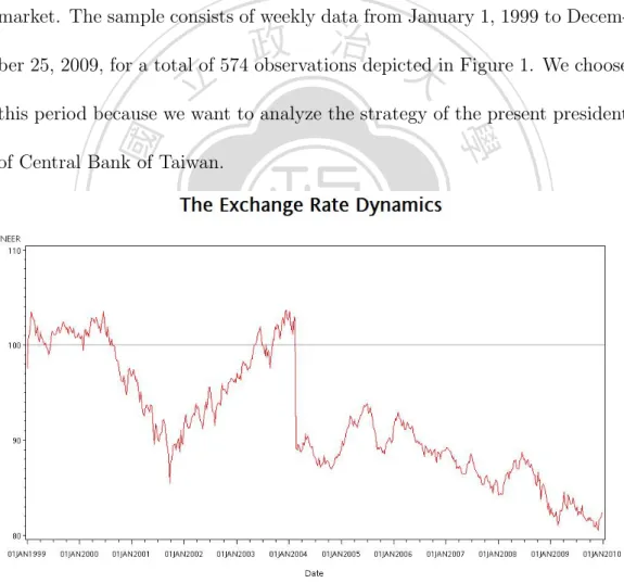
(31) 5 5.1. Empirical Results Data. We use the Nominal Effective Exchange Rate(NEER) index (2000=100) of Taiwan from Datastream, take logarithm. We use weekly data because of the possibility of day-of-the-week and week-end effects in foreign exchange market. The sample consists of weekly data from January 1, 1999 to Decem-. 政治大. ber 25, 2009, for a total of 574 observations depicted in Figure 1. We choose. 立. this period because we want to analyze the strategy of the present president. ‧ 國. 學. of Central Bank of Taiwan.. ‧. n. er. io. sit. y. Nat. al. Ch. engchi. i n U. v. Figure 1: Nominal Effective Exchange Rate Index(2000=100). 25.

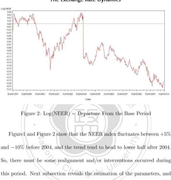
(32) 立. 政治大. ‧ 國. 學. Figure 2: Log(NEER) = Departure From the Base Period. ‧ sit. y. Nat. Figure1 and Figure 2 show that the NEER index fluctuates between +5%. n. al. er. io. and −10% before 2004, and the trend tend to head to lower half after 2004.. i n U. v. So, there must be some realignment and/or interventions occurred during. Ch. engchi. this period. Next subsection reveals the estimation of the parameters, and tries to explain the circumstances through the models to fit the data.. 5.2. Estimation. Recall that √ β1i β2i. =− =−. (1−γ)µv +. (1−γ)µv −. √. 2 [(1−γ)µv ]2 + α [(1−γ)σv ]2 2 [(1−γ)σv ] 2 [(1−γ)µv ]2 + α [(1−γ)σv ]2 [(1−γ)σv ]2. 26.

(33) β1 [e. 2 β σ2 β2 σs β (f + 22 s ) 2 ) −e 2 β σ2 β σ2 β σ2 β σ2 β1 (f + 12 s )+β2 (f + 22 s ) β1 (f + 12 s )+β2 (f + 22 s ). ]. β1 [e. 2 β σ2 β1 σs β (f + 12 s ) −eβ1 (f + 2 ) e 1 β σ2 β σ2 β σ2 β σ2 β1 (f + 12 s )+β2 (f + 22 s ) β1 (f + 12 s )+β2 (f + 22 s ). ]. eβ2 (f +. t = Asof 1 t Asof = 2. −e. −e. st = ft + α(1 − γ)µv + A1 e. β1 ft. β 2 ft. + A2 e. The following are the parameters we need to obtain A1 , A2 , β1 and β2 ,9 parameter (σs2 , γ) (0,0). 立. α. µ. σf. f. f. 政治大. 255.6038 -0.17994 -1.00784 -0.83005 5.887271 (178.5). (0.2031). (0.0105). (0.1753). (1.2748). ‧ 國. 學. After obtaining the values of A1 , A2 , β1 and β2 , we can derive the exchange rate dynamics through equation (5), Figure 3 depicts the situation of. ‧. n. er. io. sit. y. Nat. al. Ch. engchi. i n U. v. Figure 3: Exchange Rate Dynamics: Krugman model 9. The SAS code is described in Appendix F. 27.

(34) (σs2 , γ) = (0, 0) which means full credibility and marginal intervention case, and this is referred to the standard Krugman model. It is interesting that the exchange rate dynamics is flatter near the lower bound than near the upper bound. That is, the honeymoon effect is stronger when the fundamentals locate at the lower levels. In other words, when the fundamentals face negative velocity shocks, the central bank tends to intervene more. But this. 政治大. phenomenon is not obvious in Krugman model. Let us increase the effects of. 立. imperfect credibility and degree of intra-marginal intervention step by step.. ‧. ‧ 國. 學. n. er. io. sit. y. Nat. al. Ch. engchi. i n U. v. Figure 4: Exchange Rate Dynamics: Soft Edge (red⇒ σs2 = 0, orange⇒ σs2 = 1, green⇒ σs2 = 2) In Figure 4, we discuss the case with (σs2 , γ) = (0, 0)(1, 0)(2, 0). Through these curves compared to Krugman’s curve, we can easily see the phenomenon 28.

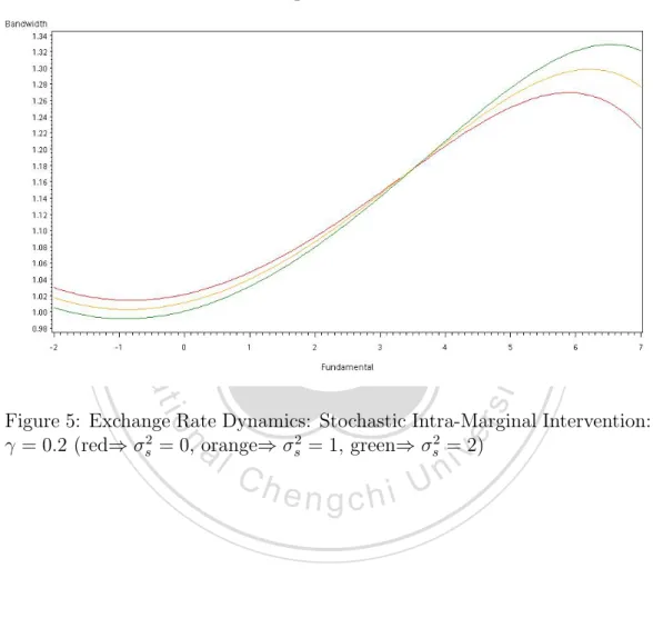
(35) described above. It is still yields a stronger honeymoon effect in the lower half. And, of course, the larger is the σs2 which means the bounds are more volatile, the wider is the zone.. 立. 政治大. ‧. ‧ 國. 學. io. sit. y. Nat. n. al. er. Figure 5: Exchange Rate Dynamics: Stochastic Intra-Marginal Intervention: γ = 0.2 (red⇒ σs2 = 0, orange⇒ σs2 = 1, green⇒ σs2 = 2). Ch. engchi. 29. i n U. v.

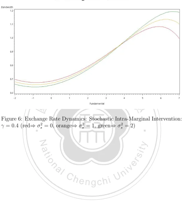
(36) 立. 政治大. ‧ 國. 學 ‧. Figure 6: Exchange Rate Dynamics: Stochastic Intra-Marginal Intervention: γ = 0.4 (red⇒ σs2 = 0, orange⇒ σs2 = 1, green⇒ σs2 = 2). n. er. io. sit. y. Nat. al. Ch. engchi. 30. i n U. v.

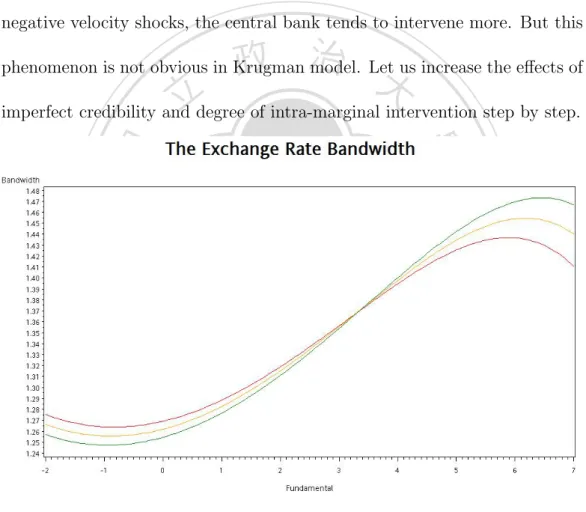
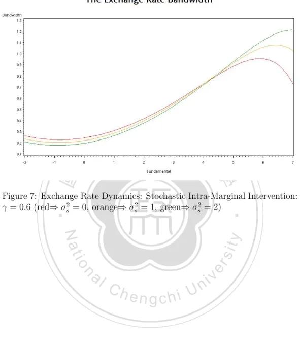
(37) 立. 政治大. ‧ 國. 學 ‧. Figure 7: Exchange Rate Dynamics: Stochastic Intra-Marginal Intervention: γ = 0.6 (red⇒ σs2 = 0, orange⇒ σs2 = 1, green⇒ σs2 = 2). n. er. io. sit. y. Nat. al. Ch. engchi. 31. i n U. v.

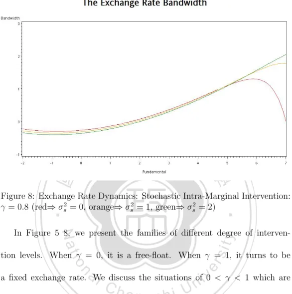
(38) 立. 政治大. ‧ 國. 學 ‧. Figure 8: Exchange Rate Dynamics: Stochastic Intra-Marginal Intervention: γ = 0.8 (red⇒ σs2 = 0, orange⇒ σs2 = 1, green⇒ σs2 = 2). sit. y. Nat. In Figure 5 8, we present the families of different degree of interven-. n. al. er. io. tion levels. When γ = 0, it is a free-float. When γ = 1, it turns to be. i n U. v. a fixed exchange rate. We discuss the situations of 0 < γ < 1 which are. Ch. engchi. more interesting. Similarly, intra-marginal intervention increases the power of honeymoon effect at the lower bound, and decrease at the upper bound. As γ increases, this effect becomes even stronger. Moreover, the extreme case in Figure 8, the exchange rates tend to mean revert at the upper half, and stay at the lower bound at the lower half.. 32.

(39) 6. Conclusion. This paper discusses the recent phenomenon of the exchange rate dynamics of Taiwan by extending Krugman model with imperfect credibility and intramarginal intervention. Through these two extensions, the target zone model is more appropriate and applicable to the case of Taiwan. First, when we observe the empirical data, we have discovered that the. 治政大 When NEER< 100, exchange rates tend to stay in the lower half recently. 立 ‧ 國. 學. it means that domestic currency is underestimated. However, this is very reasonable operation for a central bank whose country depends greatly on. ‧. exports.. Nat. sit. y. Then, we try to set up a model to fit the data. If the central bank has. n. al. er. io. no action in the zone such as Krugman model, it is hard to achieve the goal. i n U. v. to keep the exchange rate underestimated. That is, the central bank must. Ch. engchi. take a lot of actions such as realignments and large degree of intra-marginal intervetion, then the model fits the data. Although the central bank of Taiwan does not claim a explicit target zone of the exchange rate, we can summarize that there is a optimal level for the policy maker through this paper. Hence, the exchange rate of Taiwan must fluctuate within a target zone, and the honeymoon effect is much stronger at. 33.

(40) the lower bound than at the upper bound. This is why the NEER of NTD is always underestimated.. 立. 政治大. ‧. ‧ 國. 學. n. er. io. sit. y. Nat. al. Ch. engchi. 34. i n U. v.

(41) Appendices A. The Continuous-time Monetary Model. The money market equilibrium conditions at home and abroad are m(t) − p(t) = φy(t) − αi(t). (1). m∗ (t) − p∗ (t) = φy ∗ (t) − αi∗ (t). (2). 政治大. (All variables except interest rates are in logarithms.). 立. International asset-market equilibrium is given by uncovered interest par-. ‧ 國. 學. ity. i(t) − i∗ (t) = Et [s(t)] ˙. (3). ‧. The model is completed by invoking PPP. y. Nat. Substitute (1). (2) and (3) into (4), we obtain. al. (4). er. io. sit. s(t) + p∗ (t) = p(t). n. v i n C h − y (t)] + α[i(t)U− i (t)] s(t) = m(t) − m (t) − φ[y(t) engchi ∗. ∗. ∗. s(t) = m(t) + v(t) + αs(t) ˙ = f (t) + αEt [s(t)] ˙ . . . . . . . . . . . . . . . . . . . . . . . . (5) where m is the money supply and v are velocity shocks which are included in f(t) that are the monetary-model ”fundamentals”. Rewrite (5) as the firstorder differential equation Et [s(t)] ˙ −. s(t) α. = − f α(t). Take its time derivative, we yield. 35.

(42) t. s(t) ˙ = α1 e α [ dtd = − α1 f (t) +. R∞ t. τ. e− α f (τ )dτ ] +. τ 1 αt R ∞ − α e [ t e Et [f (τ )]dτ ] α2. 1 αt e α2. R∞. t. e− α Et [f (τ )]dτ. ⇒ s(t) = α1 e α. R∞ t. t. τ. e− α Et [f (τ )]dτ. τ. (6). So the exchange rate dynamics can be shown that the convergent solution to the forward-looking equation (5) has the form of an expected discounted integral of future f(t) realization.. 立. 政治大. ‧. ‧ 國. 學. n. er. io. sit. y. Nat. al. Ch. engchi. 36. i n U. v.

(43) B. Derivation of Equation(10) and (11). √A1. R∞. 2πσs2. =. λ1 f e −∞ e. √A1 2 2πσs. = √A1. R∞. −∞. R∞. −∞. 2πσs2. = A1 eλ1 (f + = A1 eλ1 (f +. (f −f )2 2 2σs. e e. df. −. 2 2f f 2 −2f f +f −2λ1 σs 2 2σs. −. 2 )]2 −(2f λ σ 2 +λ2 σ 4 ) [f −(f +λ1 σs 1 s 1 s 2 2σs. 2 λ1 σs ) 2. R∞. −∞. √1. 2 λ1 σs ) 2. 2πσs2. e. df df. 2 )]2 [f −(f +λ1 σs − 2 2σs. df. 政治大. 學. Brownian 立 motion, Wiener process, random walk. ‧ 國. C. −. ‧. Now, we introduce briefly the relevant conceptions for setting model. In applied mathematics, the Wiener process is used to represent the integral of. sit. y. Nat. io. al. n. three facts:. er. a Gaussian white noise process. The Wiener process Wt is characterized by. 1. W0 = 0. Ch. engchi. i n U. v. 2. Wt is almost surely continuous. 3. Wt has independent increments with distribution Wt − Ws N (0, t − s) , for 0 ≤ s < t. Various different types of random walk are of interest. Often, random walks are assumed to be Markov chain of Markov process. 37.

(44) D. Stochastic Calculus. Let f(t) be a continuous-time stochastic process that grows at the constant rate, µ, df (t) = µdt Let G(f(t) , t) be some possibly time-dependent continuous and differential function of f(t), then its total differential is dG =. ∂G df (t) ∂f. +. ∂G dt ∂t. 立. 政治大. ‧ 國. 學. If f(t) is a continuous-time stochastic process, the formula for total differential doesn’t work and needs to be modified. We will working with a. ‧. continuous-time stochastic process f(t) called a diffusion process where the. Nat. sit. n. er. io. df (t) = µdt + σdW (t). al. y. growth rate of f(t) randomly deviates from µ,. i n U. v. µdt is the expected change in f conditional on information available at. Ch. engchi. time t, σdW (t) is an error term and σ is a scale factor. W(t) is called a Wiener process or Brownian motion and it evolves according to √ W (t) = η t where η ∼ N (0.1). At each instant, W(t) is hit by an independent draw η from the standard normal distribution. Infinitesimal changes in W(t) can be thought of as. 38.

(45) √ √ √ dW (t) = W (t + dt) − w(t) = ηt+dt t + dt − ηt t = η˜ dt √ √ whereηt+dt t + dt N (0, t + dt) and ηt t N (0, t) √ √ E[ηt+dt t + dt − ηt t] = 0 √ √ var(ηt+dt t + dt − ηt t) = t + dt − t = dt define the new random variable η˜ ∼ N (0, 1). The diffusion process is the continuous-time analog of the random walk with drift µ. Sampling the. 政治大. diffusion f(t) at discrete points in time yields. R t+1 t. dτ + σ. 立df (τ ). R t+1 t. R t+1 t. 學. =µ. ‧ 國. f (t + 1) − f (t) =. dW (τ ) = µ + σ η˜. P |[dW (t)]2 − E[dW (t)]2 | > θ ≤. ‧. Apply Chebyshev’s inequality,. sit. y. Nat. (dt)2 θ2. io. er. Since dt is a fraction, as dt →0,(dt)2 goes to zero even faster than dt. al. does. Thus the probability that [dW (t)]2 deviates from its mean dt become. n. v i n Ch negligible over infinitesimal increments i UThis suggests that we can e n g ofc htime.. treat the deviation of [dW (t)]2 from its mean dt as an error term of order O(dt2 ). [dW (t)]2 = dt + O(dt2 ) Taking second-order Taylor expansion of G ∆G =. ∂G ∆f (t) ∂f. +. ∂G ∆t ∂t. 2. + 12 [ ∂∂fG2 ∆f (t)2 +. O(∆t2 ) 39. ∂2G ∆t2 ∂t2. 2. ∂ G + 2 ∂f (∆f (t)∆t)] + ∂t.

(46) √ where ∆f (t) = µ∆t + σ∆W (t) with ∆W (t) = η ∆t ⇒ [∆f (t)]2 = µ2 (∆t)2 + σ 2 (∆W )2 + 2µσ(∆t)(∆W ) = σ 2 ∆t + O(∆t3/2 ) ⇒ ∆G =. ∂G ∆f (t) ∂f. +. ∂G ∆t ∂t. +. σ2 ∂ 2 G ∆t 2 ∂f 2. + O(∆t2/3 ). As ∆t → 0, O(∆t2/3 ) can be ignored. dG =. ∂G df (t) ∂f. +. ∂G dt ∂t. +. σ2 ∂ 2 G dt 2 ∂f 2. 政治大. This result is known as Itˆ o’s lemma.. 立. ‧. ‧ 國. 學. n. er. io. sit. y. Nat. al. Ch. engchi. 40. i n U. v.

(47) E. Solution of Krugman’s Model. First we solve for Et [f (τ )] f (τ ) − f (t) = =. Rτ t. µdr +. Rτ t. Rτ. df (r)dr. t. σdW (r). √ = µ(τ − t) + σµ τ − t ⇒ Et [f (τ )] = f (t) + µ(τ − t) substitute into (6) ⇒ s(t) =. 1 R∞ α t. e. t−τ α. t. ‧ 國. R∞ t. τ. t. e− α dτ + µe α. R∞ t. τ. τ e− α dτ. 學. = α1 e α [f (t) − µt]. 治政大 [f (t) + µ(τ − t)]dτ 立. = f (t) + αµ. ‧. which is the no bubbles solution for the exchange rate under permanent. Nat. sit. y. free-float regime where the fundamentals follow the (µ, σ) diffusion process.. n. al. er. io. But in target zone regime, the authorities intervene infinitesimally at the. i n U. v. margin of the band. As long as the exchange rate lies within the target zone,. Ch. engchi. the authorities do nothing and allow the fundamentals to follow the diffusion process. During times of intervention, the fundamentals do not obey the diffusion process but are following some other process. So we should modified the forecasting rule to account for the fact that the process governing the fundamentals switches from diffusion to the alternative process during intervention periods.. 41.

(48) Let s(t) = G[f (t)]. By Itˆ o’s lemma, ds(t) = dG[f (t)] = G0 [f (t)]df (t) + = G0 [f (t)][µdt + σdW (t)] +. σ 2 00 G [f (t)]dt 2. σ 2 00 G [f (t)]dt 2. Taking expectation conditioned on information at time t σ 2 00 G [f (t)] 2. ˙ Et [G(t)] = µG0 [f (t)] + recall that Et [s(t)] ˙ −. s(t) α. 政治大. = − f α(t). 立. (9). G00 [f (t)] +. 2µ 0 G [f (t)] σ2. −. 2 G[f (t)] ασ 2. = − ασ2 2 f (t). y q. µ2 σ4. +. io. sit. where λ = − σµ2 ±. 2 ασ 2. er. Nat. G[f (t)] = s(t) = f (t) + µα + A1 eλ1 f (t) + A2 eλ2 f (t). ‧. The general solution is. 學. ‧ 國. substitute (8) into (9), then. al. To solve for the constants A1 and A2 , we need two additional pieces. n. v i n Ch U These are provided rules. e n gbycthe h iintervention. of information.. From the. exchange rates dynamics, we can see that the function mapping f(t) into s(t) is one-to-one. This means that there is a lower and upper bound on the fundamentals,[f , f ], that corresponds to the lower and upper bound for the exchange rates,[s, s]. When s(t) hits the upper band s, the authorities intervene to prevent s(t) from moving out of the band. Only infinitesimally small interventions are required. During the instants of intervention, ds=0,so 42.

(49) that s0 (f ) = 1 + λ1 A1 eλ1 f + λ2 A2 eλ2 f = 0 Similarly, s0 (f ) = 1 + λ1 A1 eλ1 f + λ2 A2 eλ2 f = 0 The above two equations are called the ”smooth pasting conditions”. According to the smooth pasting conditions, we can solve for the constants A1 and A2. 立. λ2 f. λ1. λ2. (λ f +λ2 f ) (λ f +λ2 f ) [e 1 −e 1 ]. e. λ1 f −eλ1 f. <0. 學. A2 =. eλ2 f −e. (λ f +λ2 f ) (λ f +λ2 f ) [e 1 −e 1 ]. ‧ 國. A1 =. 政治大 >0. ‧. λ1 is positive and λ2 is negative so that eλ1 (f −f ) > eλ2 (f −f ) . It follows that the square bracketed term in the denominator is positive.. sit. y. Nat. io. er. The solution with drift diffusion process seem to be complex. It will. al. become simpler If we add a symmetric assumption: there is no drift in the. n. v i n C h λ = −λ = λU> 0, and f = −f so that µ = 0, implies engchi. fundamentals,i.e.. 1. 2. A2 = −A1 = A > 0. Then s(t) = f (t) + A[e−λf (t) − eλf (t) ] with λ =. q. 2 , ασ 2. A=. eλf −e−λf λ[e2λf −e−2λf ]. Since market participants expect the authorities to intervene when the exchange rate heads toward the bands, the expectation of the future intervention dampens current exchange rate movements. This dampening is called 43.

(50) the ”Honeymoon effect”.. F. SAS Code. %LET nobs=574; %LET nsim=10; /*simulate the diffusion process*/ /*use Euler approximation with n=10*/ DATA tempf; alpha=1.5; sigma=3; eta= -1.4; fbar= 5; barf= -5; DO i1 = 1 to &nsim; DO i2 = 1 to &nobs; if i2=1 then f=0; else do; u=rannor(seed); lf=f; f=lf+eta+sigma*u; if f>= fbar then f=2*fbar-f-lf; else if f <=barf then f=2*barf-f-lf; else f=f; end; output; end; end; RUN;. 政治大. 學 ‧. ‧ 國. 立. n. engchi. sit er. io. Ch. y. Nat. al. DATA simf; SET tempf; if i1= &nsim then output; RUN;. i n U. v. DATA smm; MERGE simf neer; RUN; /*Simulated Method of Moments Estimation*/ /*Krugman model sigmassq=0*/ TITLE ’Simulated Method of Moments’; PROC MODEL DATA=smm; PARMS alpha 1.5 sigma 3 eta -1.4 fbar 5 barf -5; instruments f; beta1=-eta/sigma**2+sqrt(eta**2/sigma**4+2/alpha*sigma**2); beta2= -eta/sigma**2-sqrt(eta**2/sigma**4+2/alpha*sigma**2); 44.

(51) A1=(exp(beta2*fbar)-exp(beta2*(barf)))/(beta1*(exp(beta1*fbar+beta2*barf)exp(beta1*barf+beta2*fbar))) ; A2= (exp(beta1*barf)-exp(beta1*fbar))/(beta2*(exp(beta1*fbar+beta2*barf)exp(beta1*barf+beta2*fbar))) ; sims=f+alpha*eta+A1*exp(beta1*f)+A2*exp(beta2*f); eq.m1 = s -sims; eq.m2 = s**2 - sims**2; eq.m3 = s**3 - sims**3; eq.m4 = s*lag(s) -sims*lag(sims); eq.m5 = s*lag2(s) - sims*lag2(sims); FIT m1 m2 m3 m4 m5 / gmm ndraw=20; RUN;. 立. 政治大. ‧. ‧ 國. 學. n. er. io. sit. y. Nat. al. Ch. engchi. 45. i n U. v.

(52) References Beetsma, Roel M. W. J. and Van Der Ploeg, Frederick (1994), “Intramarginal interventions, bands and the pattern of ems exchange rate distributions”, International Economic Review, 35(3), 583–602. Bertola, Giuseppe and Caballero, Ricardo J. (1992), “Target zones and realignments”, American Economic Review, 82(3), 520–536. Bertola, Giuseppe and Svensson, Lars E.O. (1993), “Stochastic devaluation risk and the empirical fit of target-zone models”, Review of Economic Studies, 60(3), 689–712.. 政治大. Bessec, Marie (2003), “The asymmetric exchange rate dynamics in the ems: A time-varying threshold test”, European Review of Economics and Finance, 2(2), 3–40.. 立. ‧. ‧ 國. 學. Chen, Yu-Fu, Funke, Michael, and Glanemann, Nicole (2009), “A soft edge target zone model: Theory and application to hong kong”, BOFIT Discussion Papers, 21.. io. sit. y. Nat. Crespo-Cuaresma, Jesus, Balazs, Egert, and MacDonald, Ronald (2005), “Non-linear exchange rate dynamics in target zones: A bumpy road towards a honeymoon-some evidence from erm, erm2 and selected new eu member states”, CESifo Working Paper, 1511(6).. er. DeJong, David N. and Dave, Chetan (2007), Structural Macroeconometrics, PRINCETON UNIVERSITY PRESS.. al. n. v i n C h analysis ofUems exchange rates using a DeJong, Frank (1994), “A univariate hi n g cEconometrics, target zone model”, Journal ofeApplied 9(1), 31–45. Duffie, Darrell and Singleton, Kenneth J. (1993), “Simulated moments estimation of markov models of asset prices”, Econometrica, 61(4), 929–952. Flood, Robert P., Rose, Andrew K., and Mathieson, Donald J. (1990), “An empirical exploration of exchange rate target-zones”, NBER WORKING PAPERS, (3543). Krugman, Paul R. (1991), “Target zones and exchange rate dynamics”, Quarterly Journal of Economics, 106(3), 669–682. Lindberg, Hans and Soderlind, Paul (1994), “Testing the basic target zone model on swedish data 1982-1990”, European Economic Reveiw, 38(7), 1441–1469. 46.

(53) Mark, Nelson C. (2000), International Macroeconomics and Finance: Theory and Empirical Methods-Theory and Econometric Methods, Blackwell Publishers. Svensson, Lars E.O. (1990), “The term structure of interest rate differentials in a target zone: Theory and swedish data”, NBER Working Paper, (3374). (1992), “Why exchange rate bands? monetary independence in spite of fixed exchange rates”, NBER Working Paper, (4207). Torres, Jose L. (2000), “Stochastic intramarginal interventions in target zones”, Journal of International Financial Markets, Institutions and Money, 10, 249–262.. 政治大. Tristani, Oreste (1994), “Variable probability of realignment in a target zone”, Scandinavian Journal of Economics, 96(1), 1–14.. 立. ‧. ‧ 國. 學. Werner, Alejandro M. (1995), “Exchange rate target zones, realignments and the interest rate differential: Theory and evidence”, Journal of International Economics, 39, 353–367.. n. er. io. sit. y. Nat. al. Ch. engchi. 47. i n U. v.

(54)