國
立
交
通
大
學
網路工程研究所
碩
士
論
文
利用三階段行為分析來偵測和分類已知與未知
的惡意程式
Three-phase Behavior-based Detection and Classification of
Known and Unknown Malware
研 究 生:徐鵬凱
指導教授:林盈達 教授
利用三階段行為分析來偵測和分類已知與未知的惡意程式
Three-phase Behavior-based Detection and Classification of Known and
Unknown Malware
研 究 生:徐鵬凱 Student:Peng-Kai Hsu
指導教授:林盈達 Advisor:Dr. Ying-Dar Lin
國 立 交 通 大 學
網 路 工 程 研 究 所
碩 士 論 文
A Thesis
Submitted to Institute of Network Engineering College of Computer Science
National Chiao Tung University in partial Fulfillment of the Requirements
for the Degree of Master in Computer Science June 2013 Hsinchu, Taiwan
中華民國一百零二年六月
I
利用三階段行為分析來偵測和分類已知與未知的惡意程式
學生: 徐鵬凱 指導教授: 林盈達
國立交通大學網路工程研究所
摘要
惡意軟體已嚴重危害到網際網路的安全,近年來已有許多惡意程式防治方案 被提出。為了達到高偵測率及低時間損耗,本論文提出一個三階段行為分析技術 來偵測和分類惡意程式。前兩階段用於惡意程式偵測,第三階段用於分類惡意程 式。我們採取兩種不同方式的偵測機制,藉由兩種偵測機制的混合使用,可有效 改善偵測準確度並加速偵測流程。在第一階段,我們利用 GFI 沙盒系統和類神 經網路為每一個程式算出惡意程度的值。在第二階段,我們先從惡意程式所產生 系統呼叫序列中找出所有共同子字串,再套用貝式機率模型留下惡意行為,再利 用這些惡意行為作字串比對來偵測。在第三階段,我們先定義惡意程式類別向量, 透過餘弦相似定理計算出該樣本的相似度,再以最高相似度那個向量所代表的類 別來做分類。本論文提出之兩階段偵測與分析方法對於惡意軟體之偵測不僅可達 到 3.6%的漏判率與 6.8%的誤判率,且能正確分類超過 85.8%的已知型態的惡意 程式,此外,本方法在整體效能上亦可減少大量的執行時間。 關鍵字: 惡意程式偵測、惡意程式分類、行為分析、沙盒、系統呼叫II
Three-phase Behavior-based Detection and Classification of Known
and Unknown Malware
Student: Peng-Kai Hsu Advisor: Dr. Ying-Dar Lin
Department of Computer and Information Science
National Chiao Tung University
Abstract
In recent years, many anti-malware solutions have been proposed. To improve both detection accuracy and time efficiency for known and even unknown malware, we propose a three-phase behavior-based malware detection and classification approach, with a fast detector in the 1st-phase to filter most programs, a slow detector in the 2nd-phase, and then a classifier at the 3rd to tell the malware type. The fast detector runs programs in a sandbox to extract external behaviors fed into a trained artificial neural network (ANN) to evaluate their maliciousness, while the slow detector extracts and matches internal behaviors, i.e., the longest common substring (LCS) of system call sequences, fed into a trained Bayesian model to calculate their maliciousness. In the 3rd-phase, we define malware type vectors consisting of internal behaviors, and calculate the cosine similarity to classify malware. The experimental results show that the integrated 2-phase detection performs significantly better than any 1-phase detection alone in both detection accuracy and time efficiency. The proposed 2-phase detection scheme can achieve 3.6% in FNR and 6.8% in FPR. Besides, this approach can distinguish the known types malware from unknown samples with an accuracy of 85.8%.
III
Acknowledgement
I would like to thank all the people who have helped and inspired me during my master study.
First and foremost, I would like to express my sincere gratitude to my advisor, Prof. Ying-Dar Lin, for his patience, motivation, enthusiasm, and persistent support to my research. Without Prof. Lin’s intensive advice and guidance, this thesis would not be materialized on schedule. Besides, my deep appreciation also goes to Prof. Yuan-Cheng Lai for providing his great ideas and valuable suggestions. I also thank my coach, Dr. Chia-Yin Lee, for his invaluable time and helps with this thesis. Additionally, I thank my fellow buddies in High-speed Network Lab for making it a convivial place to work in, all the fun we have enjoyed in the past two years, and every moment we worried along.
Last but not least, I show my most cordiale thanks to my parents for giving birth to me and supporting me materially and spiritually throughout my life.
IV
Contents
List of Figures ... V List of Tables ... VI Chapter 1. Introduction ... 1 Chapter 2. Background ... 52.1 System Call and Sandbox ... 5
2.2 Related Works ... 6
Chapter 3. Problem Statement ... 9
3.1 Definition of Notations ... 9
3.2 Problem Description ... 10
Chapter 4. three-phase Behavior-based Analysis ... 11
4.1 Approach Overview ... 11
4.2 Sandbox-based Detection mechanism ... 12
4.3 System Call-based Detection mechanism ... 14
4.4 Behavior-based Classifier ... 17
Chapter 5. Evaluation... 20
5.1 Experiment Environment ... 20
5.2 Experimental Results ... 24
Chapter 6. Conclusions and Future Works ... 33
V
List of Figures
Figure 1. The relationship among different behaviors ... 2
Figure 2. The system overview ... 11
Figure 3. Architecture of SDM ... 13
Figure 4. Distribution for capability of detection. ... 13
Figure 5. Architecture of SCDM. ... 15
Figure 6. Architecture of behavioral classifier. ... 18
Figure 7. Type training flow. ... 19
Figure 8. Example for type training flow... 19
Figure 9. Experiment environment of SDM. ... 21
Figure 10. Distribution for suspicious behaviors from the GFI sandbox. ... 22
Figure 11. Architecture of the system call tracer. ... 22
Figure 12. How to record system calls... 23
Figure 13. Distribution for MD values. ... 25
Figure 14. Detection ratio with different MD values. ... 25
Figure 15. Detection ratio with different lengths as threshold. ... 26
Figure 16. Distribution for the number of malicious behaviors... 27
Figure 17. Detection: 1-phase v.s. 2-phase. ... 29
Figure 18. Classification for malware of known types and unknown types. ... 30
VI
List of Tables
Table 1. Related works on anti-malware solution ... 6
Table 2. Notations used in the proposed scheme ... 9
Table 3. Detection ratio v.s. Time cost. ... 27
Table 4. Decision on 1st-phase. ... 28
Table 5. Identification for malware with or without intrusions. ... 31
1
Chapter 1 Introduction
Malware is a collective term for a variety of malicious-purpose software that could execute on a computer system without an administrator’s authorization. Recently, a large amount of profit-oriented malware has been utilized to steal sensitive information or to launch attacks against a victim. It might result in the financial loss and resource waste. Therefore, many anti-malware solutions have been proposed for preventing malware infection.
Signature-based vs. Behavior-based
Existing anti-malware solutions can be categorized into two types, i.e., signature-based scanning, which has light computation overhead, and behavior-based analysis, which has heavy computation overhead. Signature-based solutions extract the unique digests of malware to construct a database of signatures. Then, these solutions can check whether a file is malicious or not by matching the binary of the file with the malware signatures. Although signature-based detection mechanisms are efficient and effective to recognize the known malware, they might fail to identify
unknown or metamorphic malware. To conquer this drawback, the behavior-based
solutions were proposed. Since malware have some common behaviors, we could use such common behaviors to judge whether a suspicious file is malicious. Thus, behavior-based solutions outperform in detecting unknown or metamorphic malware.
Host Behaviors vs. Network Behaviors
In general, we can observe malware’s behaviors in two different aspects: host behaviors and network behaviors. Host behaviors refer to all the activities that might change attributes of the system, such as modifying the registry files of the operating system (OS). On the other hand, network behaviors usually make connections to
2
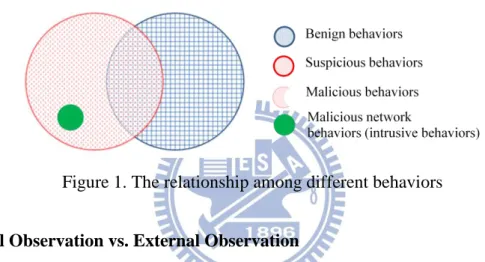
remote victims or servers, such as command and control (C&C) servers. Figure 1 illustrates the relationship among different behaviors. Benign programs have only
benign behaviors (BB) while malware exhibits suspicious behaviors (SB) which
contain both benign behaviors and malicious behaviors (MB). Malware might make use of benign behaviors to shelter its malicious ones. Most of the malware have malicious host behaviors; however, only some kinds of the malware have additional malicious network behaviors, i.e., intrusive behaviors (IB), to influence remote victim hosts, where IB
MB.Figure 1. The relationship among different behaviors
Internal Observation vs. External Observation
Many behavior-based anti-malware solutions investigate malware’s behaviors by
internal observation or external observation. For internal observation, it can trace the
processes of the OS by interrupting the execution or checking the registers to record some footprints, such as system calls. Forrest et al. [1], Mutz et al. [2], and Warrender et al. [3] proposed methods to record the normal system call sequences so as to detect anomalous behaviors. Lin et al. [4] built system call sequences as behaviors, and applied Bayes’ theorem to calculate the malicious degree (MD) of evaluated programs. Lin et al. [5] recognized obfuscated bots by calculating the longest common subsequence similarity between system call sequences. Rozenberg et al. [6] dealt with system call sequences in fixed length by SPADE [7] sequence mining methodology. Moreover, there existed other solutions, such as Cha, et al.’s [8], Li, et al.’s [9], and
3
Mehdi et al.’s [10] schemes, which try to link up system calls with the soundex algorithm, sequence alignment, and genetic algorithm, respectively.
On the other hand, examining malware by external observation is from a macroscopic point to observe the aggregated activities of malware, such as modifying files. Liu et al. [11] proposed a mechanism that it defines malicious behavior features (MBF), and evaluates the malware with the MBF. Recently, Tsai and Wang [12] proposed an effective malware detection scheme, called ANN-MD, to obtain the representative behaviors of the malware using three well-known sandboxes. In addition, they employed artificial neural networks (ANN) to calculate the malicious degree (MD).
Both internal and external observations can help us to find malware’s trail; however, they still have some limitations. Internal observation provides a much more
fine-grained way to diagnose symptoms of malware, but makes it more time-consuming to dissect malware. In contrast, external observation attracts us with
its rapid examination but leaves us coarse-grained inspection. In order to improve the detection accuracy and time efficiency, we could adopt both internal and external observations to design a hybrid approach against malware.
A Three-phase Approach
We evaluated the time cost of external and internal observations with some experiments conducted. The external observation, such as using sandboxes with artificial neural networks to observe malware behaviors, would take about 3 minutes. The time cost of the internal observation, such as using system call approaches with longest common substring (LCS), takes approximately 15 minutes. In this work, we deploy the external observation in the 1st-phase and internal observation in both 2nd-phase and 3rd-phase. In the 1st-phase, we use a sandbox to obtain all behaviors,
4
and then calculate the MD values for each to-be-detected program by using artificial neural network. In the 2nd-phase, we discover some common behaviors between different malware by extracting the longest common substring of system call sequences, and then employ Bayes probabilistic model to check the likely malicious behaviors. While detecting, the 2nd-phase only processes the to-be-detected programs which are not caught by the 1st-phase. In the 3rd-phase, Based on those malicious behaviors, we can recognize different kinds of malware.
The rest of this thesis is organized as follows. In Chapter 2, we first review some related works, and then compare existing schemes with ours. In Chapter 3 and Chapter 4, we give the precise problem statement and describe the structure of the proposed scheme in detail, respectively. In Chapter 5, experimental results are presented to validate the functionality and the performance of the proposed scheme. Finally, some concluding remarks and future work are given in Chapter 6.
5
Chapter 2 Background
In this chapter, we describe the key technologies used in the proposed scheme. Moreover, some related works are also discussed and compared in this chapter.
2.1 System Call and Sandbox
System Call
System calls are a kind of function calls implemented by the OS kernel. They provide an essential interface between a process and OS. Processes in a system are run in different modes. The processes run in the user mode have no access to the privileged instructions. If they need any services, they must request the kernel of OS for the services through system calls.
Attackers usually embed the malicious codes into benign programs, and then spread these compromised programs around through the Internet. Even though malware can masquerade in various appearances, it is the invocations of the system calls that the malware cannot alter while doing its critical actions. The series of system calls issued from the same kind of malware resemble each other considerably, and thus we could follow the trail of a program to identify malware by its system call
sequence.
Sandbox
A sandbox is a virtualized platform which provides a tightly controlled set of resources and an isolated environment for executing a suspicious program. The sandbox can process interactive procedures with malware. Therefore, the malware can do whatever it wants, such as modifying or deleting files, duplicating several copies to compromise the system, connecting to malicious servers, and downloading files. It is worth noting that above actions will affect neither the host system nor the machines in
6
the Internet. Further, the runtime behaviors of the suspicious program can be recorded by the sandbox. In fact, the sandbox is a popular and effective tool to discover behaviors of malware.
2.2 Related Works
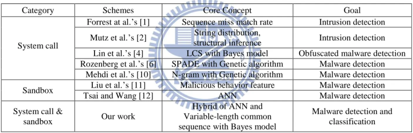
In order to overcome the drawback of signature-based anti-malware solutions, many behavior-based anti-malware solutions have been proposed. In this section, we review some related works for malware and intrusion detection with their flaws pointed out, and then propose an improvement. Some related works are summarized in Table 1.
Table 1. Related works on anti-malware solutions
Category Schemes Core Concept Goal
System call
Forrest at al.’s [1] Sequence miss match rate Intrusion detection Mutz et al.’s [2] String distribution,
structural inference Intrusion detection Lin et al.’s [4] LCS with Bayes model Obfuscated malware detection Rozenberg et al.’s [6] SPADE with Genetic algorithm Malware detection
Mehdi et al.’s [10] N-gram with Genetic algorithm Malware detection Sandbox Liu et al.’s [11] Malicious behavior feature Malware detection
Tsai and Wang [12] ANN Malware detection
System call &
sandbox Our work
Hybrid of ANN and Variable-length common sequence with Bayes model
Malware detection and classification In 1996, Forrest et al. [1] proposed a method to record the series of normal system calls by some benign programs into the database. When a compromised program executes malicious codes, the anomalous system call sequence patterns can be detected because those patterns do not exist in the database. Later on, many system call-based approaches [3][8][13] have been proposed. In 2006, Mutz et al. [2] identified anomalous behaviors by system calls with different considerations: string length rarely exceeds a hundred characters and consists of human-readable characters; string character distribution is based on the observation that strings have a regular structure and almost always contain only printable characters; token finder determines
7
whether the values of a certain system call argument are drawn from a limited set of possible alternatives, i.e. elements of an enumeration. These two anomaly-based detection methods should accumulate normal behaviors with large-scale experiments, or theirs would introduce high false positive rate. Besides, attackers might evade those defenses.
Recently, Mehdi et al. [10] came up with a solution, named IMAD, to obtain sequential system call in fixed length using N-gram segmentation model. This solution discriminates malicious behaviors from benign ones by checking whether the system call sequence is only invoked by malware, and gives the system call sequence a goodness value. If the sequences invoked by both malware and benign programs, it will evaluate their goodness by genetic algorithm. Those goodness values can be used to calculate an overall impression value of a process. The higher impression value of a process gets the stronger probability the process is declared as benign. Later, Rozenberg et al. [6] tackled system call sequences with SPADE sequence mining methodology and genetic algorithm. Those system call sequences invoked only by malware are reserved for later detection. The common shortcoming that both methods view system call sequences in fixed length becomes their Achilles’ heel, because different malicious behaviors might invoke various quantities of system calls.
Lin et al. [4] extracted longest common system call substrings among the same types of malware to represent behaviors. Afterwards, they employed Bayes probability model to assign a value for each behavior. This value indicates the maliciousness and can be used to detect obfuscated programs. Although this method handled variable-length system call sequences, it inclined to missing a lot of sequences owing to their extraction procedure that there is always only one longest common subsequence (LCS) between two system call sequences.
8
feature (MBF) of malware by observing processes of Windows systems and then
using the MBF to detect the malware, where MBF is a three-tuple, i.e., Feature_id, Mal_level, and Bool_expression. Note that Feature_id is a string identifier which is used to uniquely represent an MBF; Mal_level divides an MBF into three malicious levels: high, warning, and low; Bool_expression is a Boolean expression which specifically defines the behavior of an MBF. The MBF can be used to calculate the malicious degree of a suspicious program. If the program conforms to more MBFs, it would be a malware with a higher probability. Tsai and Wang [12] utilized three sandboxes, i.e., GFI sandbox [14], Norman sandbox [15], and Anubis sandbox [16], to obtain representative behaviors of a program. They selected 13 behaviors that malware frequently carry out but rarely do benign programs. Finally, this method constructed a MD expression by using ANN for malware detection. However, these two methods, of which one declared only 3 malicious levels and the other considered
only those behaviors related to malware, lack precise inspection.
Sandbox-based approach makes it faster to analyze a program, and system call-based approach analyzes a program in finer-grained way. To combine strong points of both schemes, we propose a hybrid system. In the faster 1st-phase, we rely on a sandbox to obtain suspicious behaviors and then adopt ANN to compute the MD value. In the slower 2nd-phase, all common system call sequences are dug out by the recursive LCS sequence mining method, and more likely malicious common system call sequences are identified by the Bayes probability model. During the detection stage, only those to-be-detected programs which are not caught by the 1st-phase are processed. In the 3rd-phase, we define type vectors to recognize the malware of known types or an unknown type. We also differentiate between intrusive malware and non-intrusive malware via its exhibited behaviors.
9
Chapter 3 Problem Statement
In this chapter, we first define some notations used in this work and then illustrate the problem statement in a formal manner.
3.1 Notations
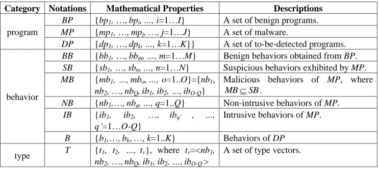
There is a set of samples containing benign programs (BP) and malware programs (MP) for training. We use BB to denote the benign behaviors obtained from benign programs and SB to signify suspicious behaviors exhibited by malware. Malicious behaviors (MB) reside in SB as a subset to indicate the harmful actions done by malware. MB consists of two kinds of behaviors, i.e., non-intrusive behaviors (NB) and intrusive behaviors (IB). For classification, we define a set of type vectors (T) to keep track of the malicious behaviors that each malware type carries. Finally, we collect numerous to-be-detected programs (DP), whose behaviors are denoted as B, to verify the effectiveness of the proposed scheme. Those notations and their mathematical properties are described in Table 2.
Table 2. Notations used in the proposed scheme
Category Notations Mathematical Properties Descriptions
program
BP {bp1, …,bpi,…, i=1…I} A set of benign programs.
MP {mp1, …,mpj,…, j=1…J} A set of malware.
DP {dp1, …,dpk,…, k=1…K}} A set of to-be-detected programs.
behavior
BB {bb1, …,bbm,…, m=1…M} Benign behaviors obtained from BP.
SB {sb1, …,sbn,…, n=1…N} Suspicious behaviors exhibited by MP.
MB {mb1, …,mbo,…, o=1..O}={nb1,
nb2, …,nbQ,ib1, ib2, …,ibO-Q}
Malicious behaviors of MP, where
SB MB . NB {nb1,…,nbq,…, q=1..Q} Non-intrusive behaviors of MP. IB {ib1, ib2, …, ibq’ , …, q’=1…O-Q} Intrusive behaviors of MP. B {b1,…,bk,…, k=1..K} Behaviors of DP type T {t1, t2, …, tv}, where tv=<nb1, nb2, …,nbQ, ib1, ib2, …,ibO-Q >
10
3.2 Problem Description
In order to recognize malware, we collect various training samples and design an approach to extract representative malicious behavior patterns. Later on, an unknown program is analyzed based on the representative malicious behavior patterns. We illustrate the problem more precisely as follows.
Given a set of BP, a set of MP, and a set of DP, in the training process, we need to obtain BB and SB from BP and MP, respectively. Next, we need to use both SB and
BB to deduce MB, whereMBSB, use MB to define T, and divide MB into NB and
IB. In the detection and classification process, our objectives are to judge whether a
given dpk is malware by MB; if yes, classify dpk into a known type or an unknown
11
Chapter 4 three-phase behavior-based analysis (TBA)
In this chapter, we describe the detailed procedure of the proposed approach. In Section 4.1, the architecture overview is depicted. In Section 4.2 and Section 4.3, we illustrate the sandbox-based detection mechanism and system call-based detection mechanism, respectively. We describe behavioral classification in Section 4.4.
4.1 Approach Overview
Considering both detection accuracy and time cost, we propose a three-phase approach with the front two phases serving detection and the rear phase serving classification. There are two different detection mechanisms adopted: sandbox-based detection mechanism (SDM) and system call-based detection mechanism (SCDM). SDM provides a faster way to observe a program, while SCDM observes a program in finer-grained way and achieve better detection accuracy. Figure 2 shows the architecture of the proposed approach. The proposed three-phase behavior-based analysis is deployed with SDM in the 1st-phase, SCDM in the 2nd-phase, and
behavioral classifier in the 3rd-phase.
Behavioral Classifier System call-based detection mechanism
(SCDM)
Sandbox-based detection mechanism (SDM) 1st tier 3rd tier 2nd tier dpk Suspicious program Malware Known type or Unknown type
12
Each sample dpk must be passed through SDM. If SDM judges a program as
suspicious, that program would be sent to SCDM for further examination. Finally, the
intrusive or non-intrusive malware is also identified according to its exhibited behaviors. Note that there are two processing flows in our approach, i.e., training flow and detection and classification flow. For the training flow, we target at digging out the MB together with IB by using BP and MP, and then define T depending on the MB. For the detection and classification flow, it is our goal to detect and classify malware by using MB and T. The detection or classification flow is processed after the training flow is done.
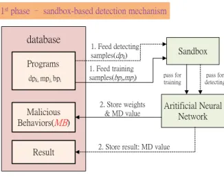
4.2 Sandbox-based detection mechanism (SDM)
As the flows shown in Figure 3, we first submit samples to a sandbox for training, and collect all corresponding runtime behaviors from the sandbox. Next, we select representative behaviors by calculating their appearance frequency. Afterward, an ANN algorithm is employed to adjust the weight of each behavior dynamically. At the end of this stage, an MD expression is constructed and two MD values can be obtained as the thresholds, upper bound and lower bound. In Figure 4, we can see that the capability of distinguishing between malware and benign samples at two ends of the double-headed arrows are relatively better. There are a few samples falling into the middle of the distribution, named as the ambiguous area.
The detection flow is to assess whether a given sample is malware. By the same way, we can collect the runtime behaviors and calculate the MD values of each program. According to the MD expression which was constructed in the training flow, we can judge this program by the MD value. If the value is larger than the upper bound, this program will be judged as malware. If the value is lower than the lower bound, it will be judged as benign. For those suspicious samples whose values fall
13
into the ambiguous area, SCDM should take over their processing from SDM.
Training flow Detecting flow database Programs dpk, mpj, bpi Malicious Behaviors(MB) Sandbox Aritificial Neural Network 1. Feed training
samples(bpi,mpj) pass for training
2. Store weights & MD value 1. Feed detecting samples(dpk) pass for detecting
2. Store result: MD value
1st phase – sandbox-based detection mechanism
Result
Figure 3. Architecture of SDM
Figure 4. Distribution for capability of detection
Suspicious Behaviors
As mentioned above, we rely on a sandbox to obtain all behaviors, and determine the representative behaviors by calculating their appearance frequency. We consider the appearance frequency with not only malware but also benign programs. The more frequent a behavior is carried out by malware, the more suspicious that common behavior is. In contrast, if only benign programs exhibit a certain behavior frequently, we can conclude that this common behavior is nothing but a normal behavior of programs. For those behaviors that malware and benign programs rarely practice, we kick them out because they provide little information for us. Finally, we keep the behaviors which conform to the above inference as representative behaviors.
14
An artificial neural network (ANN) [17] is one kind of machine learning algorithm in the field of Artificial Intelligence. An ANN is composed of several interconnected artificial neurons. Each neuron of ANN can receive data from multiple inputs and perform a local computation. Besides, the output of a neuron is determined by an activation function. In this work, we employ feed-forward ANN to cluster malware and benign software. We adopt 12 representative behaviors of dpk as the
input neurons of ANN, and then, we can get the MD value after a complicated computation.
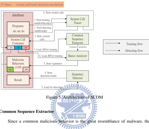
4.3 System call-based detection mechanism
As illustrated in Figure 5, SCDM contains four modules and a database. The
System Call Tracer can trace programs’ trails by recording their issued system calls
and then construct SB, BB, and B. The Common Sequence Extractor can observe programs’ common behaviors by mining all common system call substrings. Afterward, the Bayes Analyzer investigates those common behaviors by the Bayes probability model together with BB to put the likely malicious common system call substrings as MB. Then, the Sequence Detector evaluates dpk by comparing dpk’s
system call sequences with MB. The database is served as a storage pool for SB, BB, B, and MB.
System Call Tracer
As discussed in Chapter 2, malware cannot alter the invocations of system calls while doing some critical actions. Hence, for all of programs to be analyzed in BP,
MP, and DP, we can execute each program individually to record the runtime-issued
system calls. For each system call, we only apply the name of it. The recorded system calls for each process are ordered by timeline to form a system call sequence. Then,
15
the system call sequence can be regarded as the trail of bpi, mpj, ordpk, and be stored
in BB, SB, or B, respectively. Training flow Detecting flow database Programs dpk, mpj, bpi System Call Container Malicious Behaviors (MB) Result NB B BB SB IB System Call Tracer Common Sequence Extractor Bayes Analyzer Common properties Sequence Detector 1. Feed training samples(bpi,mpj) 2. Store system calls
4. Load BB for training 5. Store signatures 1. Feed detecting samples(dpk)
3. Load for detecting 2. Store system calls
4. Store detection results
2nd phase – system call-based detection mechanism
3. Load SB for training
Figure 5. Architecture of SCDM
Common Sequence Extractor
Since a common malicious behavior is the great resemblance of malware, the system call sequences recorded from the malware should share the system call
subsequences considerably. We would like to find out common subsequences of
malware and use them to represent malicious behaviors. LCS is a sequence mining algorithm for extracting the longest common consecutive subsequence, also named as substring. For any two sequences, only one LCS can be extracted. In order to dig out more common substrings, we recursively extract the LCS between any two sequences as
where denotes the length of ’s system call sequence. Then, we can deduce
16
where and signify the i-th and j-th positions in ’s system call sequence, respectively. means the ’s system call substring, starting at position and terminated at position of ’s system call sequence. represents all the common
substrings of and .
refers to the LCS, which is extracted between
and . Finally, we can dig out all common substrings
between any two sequences. Whenever mpj is fed into the extraction
procedure, we can extract all common substrings between any two pieces of malware.
Bayes Analyzer
We gain a lot of system call substrings after the extraction procedure. Not all of them can be guaranteed as the malicious behaviors because malware might exhibit both benign behaviors and malicious behaviors. Accordingly, we have to evaluate every extracted substring in terms of the probability of appearance under the Bayes probability model. The Bayes probability formula is calculated as
where sbn is the extracted system call substring to be evaluated. P(B) denotes the
probability that the given programs are benign programs while P(M) denotes the probability for malware. P(sbn|B) and P(sbn|M) represent the probability that the sbn is
carried out by benign programs and malware, respectively. Then, we can get the probability P(M|sbn) which implies the probability of a program being malware given
the condition that the program practiced sbn. Based on Lin et al.’s experiment [4], the
17
behavior. Since intrusive behaviors are only exhibited by intrusive malware, we also label mbo with its owner to tell the intrusive behaviors apart. Finally, the MB and IB
are obtained.
Sequence Detector
As mentioned above, the calculated probability of mbo is 1. It is inferred that
only malware carries out mbo. This also makes the detection procedure more
simplified. For each dpk, we first record its runtime-issued system call sequence as bk,
and then compare the bk with all elements in MB. Once bk matches mbo, dpk is
esteemed to be malware.
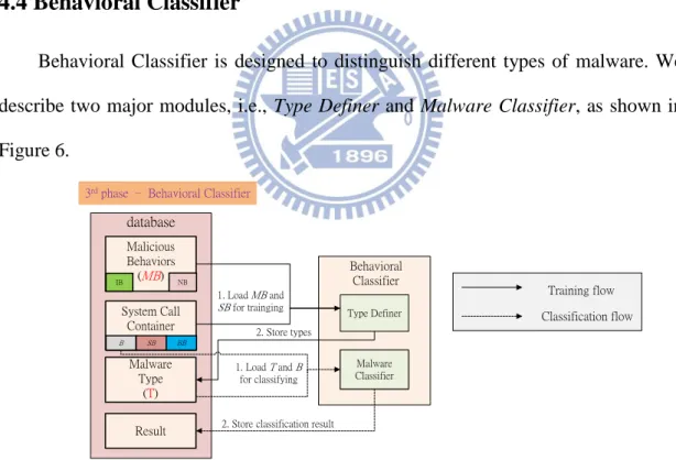
4.4 Behavioral Classifier
Behavioral Classifier is designed to distinguish different types of malware. We describe two major modules, i.e., Type Definer and Malware Classifier, as shown in Figure 6. Training flow Classification flow database Malware Type (T) Malicious Behaviors (MB) IB NB Type Definer Result Behavioral Classifier Malware Classifier 2. Store types 1. Load T and B for classifying
2. Store classification result
3rd phase – Behavioral Classifier
Malware Classifier 1. Load MB and SB for trainging System Call Container B SB BB
Figure 6. Architecture of behavioral classifier
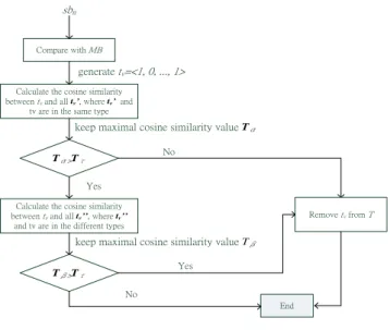
Type Definer
We use a type vector tv to represent a type of malware, where tv is defined as
18
Type vectors are identified with O-tuple of binary numbers, where the symbol ‘0’ denotes the absence of mbo, and the symbol ‘1’ denotes the presence of mbo. A type
vector tv is built by noting down what malicious behaviors a piece of malware
performs. Subsequently, in order to make sure that each tv is guaranteed to resemble
the vector of the same type as tv but differ from the vectors of the other types. As
shown in Figure 7, we first calculate the cosine similarity [18] between tv and the
other type vectors tv’ which represent the same type as tv. The cosine similarity is
obtained by ‧
where tv and tv’ are two of type vectors. According to formula (4), all the calculated
similarity values are between 0 and 1. The more the calculated similarity value is, the more similar two type vectors are. We keep the calculated maximal similarity value
Tα and set a value as the threshold Tτ to determine whether to disable the exerciseof tv. If the Tαis lower than the Tτ , tv will be disabled. Then, we calculate the cosine
similarity between tv and all the other type vectors, tv’’, which represent different
types from tv, and then keep the calculated maximal similarity value Tβ. If the Tβ is
lower than the Tτ , tv will be put into practice. In this way, we can construct a set of
type vectors, T, for classification. The above training flow is depicted in Figure 7. In Figure 8, we assume that t1, t2, and t3 represent type1 while t4, t5, and t6
represent the other types, and the threshold is set as 0.5. We train t3 by first
calculating the cosine similarity between t3 and t1, t3 and t2. Then, we can get maximal
similarity value 0.65, which is calculated between t3 and t2. Because 0.65 is greater
than the threshold (0.5), we then calculate the cosine similarity between t3 and t4, t3
and t5, t3 and t6. We can get another maximal similarity value 0.6, which is calculated
19 be used.
Compare with MB
Tα>Tτ sbn
Calculate the cosine similarity between tv and all tv’, where tv’ and
tv are in the same type
generate tv=<1, 0, ..., 1>
keep maximal cosine similarity value Tα
End
No
Calculate the cosine similarity between tv and all tv’’, where tv’’
and tv are in the different types
Yes
keep maximal cosine similarity value Tβ
Remove tv from T
Tβ>Tτ
Yes No
Figure 7. Type training flow
t1=<1, 1, …, 1>
t2=<0, 1, …, 1>
t3=<0, 0, …, 1>
Maximal similarity with type vectors which represent the
same type as tv
(type vector → value)
t2 → 0.65
Type 1
t6 → 0.6
threshold=0.5
Maximal similarity with type vectors
which represent different types from tv
(type vector → value)
t4=<1, 0, …, 0>
t5=<1, 0, …, 1>
t6=<0, 1, …, 0>
Other types
Figure 8. Example for type training flow
Malware Classifier
We also build a vector for each dpk to keep track of its exhibited malicious
behaviors, and then calculate the cosine similarity between dpk’s vector and all type
vectors in T. We classify dpk into the type that tv represents, where the calculated
similarity between dpk’s vector and tv is the greatest. In addition, a threshold is also
set as the lower bound for the calculated similarity to determine whether the dpk
belongs to a known type or an unknown type. Note that if we want to classify the malware caught by SDM, we should collect the runtime-issued system calls of that malware by System Call Tracer.
20
Chapter 5 Evaluation
We design various experiments to verify the effectiveness of the proposed scheme and discuss experimental results. In Section 5.1, we present the experiment environment and the system configuration. In Section 5.2, we investigate several issues with corresponding experimental results drawn, and then interpret these results with great insight.
5.1 Experiment environment
We clarify the configurations and environments in three parts: programs, SDM, and SCDM.
Programs
We collect 1800 executable programs as the sample space. These 1800 programs comprise 1000 malicious programs and 800 benign programs, with 900 programs (500 malicious programs and 400 benign programs) for training and detection, separately. Note that malware samples are collected from VX Heaven [21] websites. The benign programs are collected from the Windows OS system directories and the CNET.com [22] website. All benign programs are guaranteed by several anti-virus tools [23]. In addition, we use some known types of malware, including Backdoor, Bot, Hoax, Trojan, Worm, etc., to evaluate the proposed classification methodology.
SDM
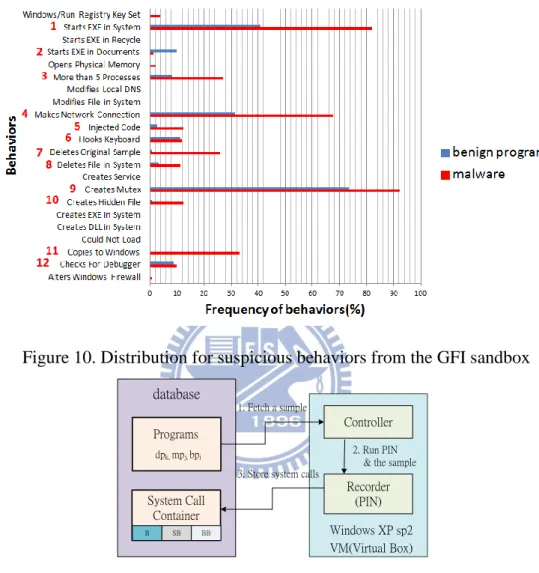
As shown in Figure 9, we utilize the GFI sandbox to obtain 22 suspicious behaviors, where the frequency for each behavior is illustrated in Figure 10. We observe that some behaviors are frequently carried out by either malware or benign programs, such as Copies to Windows and Starts EXE in Documents, while there are
21
some behaviors that both malware and benign programs practice, such as creates mutex. We eliminate those behaviors that malware and benign programs rarely perform, such as Opens Physical Memory and Modifies Local DNS. Finally, only 12 representative behaviors are kept, where their appearance frequencies of malware or benign programs are above 5%. The representative behaviors include Starts EXE in System, Starts EXE in Documents, More than 5 Processes, Makes Network Connection, Injected Code, Hooks Keyboard, Deletes Original Sample, Deletes File in System, Creates Mutex, Creates Hidden File, Copies to Windows, Checks for Debugger. We utilize Pattern Recognition Tool in Matlab 8.0.0 to implement the ANN system. The input layer of the ANN consists of 12 representative behaviors. We also adopt the built-in function initnw to distribute the initial weight for each neuron. By serial calculation, ANN finally can generate an MD value for each sample.
GFI sandbox Sandbox
Database
Programs ContainerBehavior
SB1
1. Feed programs in 2. store 12 behaviors
3. Feed in for
detecting ANN
Matlab
Figure 9. Experiment environment of SDM
SCDM
System Call Tracer comprises two components. One is the Controller, and the other is the Recorder. The Controller can coordinate the execution and recording environment. It fetches a program from the database, and then executes the program with the Recorder. The Controller is also responsible for the integrity of the recording environment. Before a program is processed, the Controller should restore the snapshot to preclude the possibility that a program is influenced by the other
22
programs’ execution results. The Recorder captures all the issued system calls of the fetched sample by the PIN tool [19]. Figure 11 illustrates the architecture of the System Call Tracer.
Figure 10. Distribution for suspicious behaviors from the GFI sandbox database Programs dpk, mpj, bpi System Call Container B SB BB Controller Recorder (PIN) 1. Fetch a sample 2. Run PIN & the sample 3. Store system calls
VM(Virtual Box) Windows XP sp2
Figure 11. Architecture of the System Call Tracer
Dynamic analysis of an executable program can be implemented in three popular ways. This first one is API hooking, in which system calls are intercepted and recorded by the hook function. However, API hooking might be detected by inspecting the Export Address Table (EAT) and Import Address Table (IAT). Therefore, malware with anti-analysis mechanisms could hide its execution to evade the API hooking. Another method is utilizing an emulator to monitor the malware. Because the whole system is emulated, the monitoring can be done in fine-granularity
23
at instruction-level. However, this method has the constraint on the inevitability to modify the source of an emulator, which implies that there is no choice but using an open-sourced emulator like QEMU [20]. The other one is the binary code instrumentation that we adopt in this work. This approach does not involve API hooking and runs much faster than the emulator-based approach as most of the time the binary is executed directly on the processor hardware. Binary code instrumentation can dynamically instrument the monitoring codes into a runtime binary whenever a certain condition is reached, e.g., a system call is about to be invoked. Figure 12 portrays how it works.
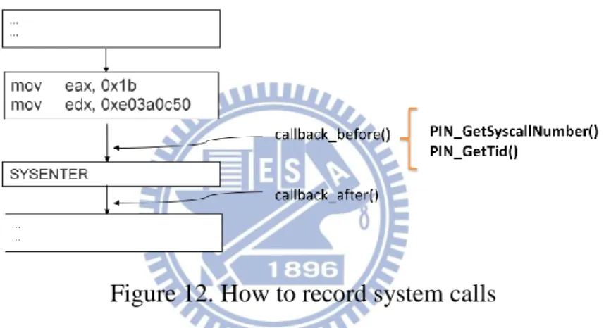
Figure 12. How to record system calls
When a program wants to invoke a system call, it puts the system call ID in the register EAX and the address of argument in register EDX. The program then uses the SYSENTER instruction to invoke the syscall handler in the OS kernel. The just-in-time compiler of PIN can monitor the SYSENTER instruction. We register a function to PIN by PIN_AddSyscallEntryFunction() API at callback_before, so that the Recorder can know the moment that the program invokes a system call. The PIN API provides us the information including the thread ID, system call ID, and the system call arguments. We only pull out some information of the system call, reserving the thread ID and system call ID while ignoring the system call arguments.
24
5.2 Experimental results
We present our results in terms of four metrics, i.e., true positive ratio (TPR), true negative ratio (TNR), false positive ratio (FPR), and false negative ratio (FNR). TPR and TNR denote the ratio that we truly identify malware and benign programs, respectively. FPR and FNR mean that benign programs or malware are mistaken. Following on, we probe into 7 issues that help us resolve doubts and introduce us into a deeper comprehension regarding this research. First, we examine the detection performance for SDM and SCDM working alone. Then, we measure the time cost for SDM as well as SCDM and compare three strategies that two detection mechanisms serve in different phases. Finally, we present the results for malware classification and intrusive malware recognition.
Impact of MD on ANN
This experiment evaluates sandbox-based detection ability. As discussed above, we can get the MD value for each program using the ANN. In order to delimit the ambiguous area and determine the optimum MD value, the distribution for MD values is shown in Figure 13.
There is an obvious ambiguous area from 0.2 to 0.75. We observe that SDM cannot discriminate malware and benign programs within the ambiguous area while SDM can tell them apart well outside the ambiguous area. Therefore, we illustrate detection ratio with different MD values in Figure 14.
In Figure 14, we set different MD values as thresholds to evaluate the detection ability. We observe that FNR goes up sharply within two intervals, i.e., from 0.2 to 0.25 and from 0.4 to 0.5. We look into the cause of the trend and notice that a large quantity of benign programs and malware practice the same suspicious behaviors. So, their calculated MD values would be similar. It might result from the capability of the
25
GFI sandbox that cannot dissect programs in a fine-grained way. If we want to keep the FNR less than 10%, the best MD threshold is 0.4.
Figure 13. Distribution for MD values by ANN
Figure 14. Detection ratio with different MD thresholds
Impact of Length on System Call Sequence
In this experiment, we evaluate the system call-based detection approach. There are a lot of variable-length system call sequences in our MB. Different system call sequences represent different malware’s behaviors. Generally, the longer system call sequence can represent malware’s common behavior more specifically, and Figure 15
26 clarifies it.
Figure 15. Detection ratio with different lengths as thresholds
We use different lengths of system call sequences as thresholds to conduct the experiment. Only the length of a system call sequence is longer than the configured threshold will it be put into use for malware detection. Figure 15 shows that there is a remarkable decrease for FPR as the length of system call sequences goes from 10 to 50. Besides, a slight variation occurred for both TPR and FPR when the length of system call sequences is greater than 50. We also discuss the issue of misjudgment. The FNR might be ascribed to the hidden malicious behaviors or the lack of triggered events. The FPR might arise from the impure MB where some benign behaviors are
not filtered out. Thus, we must collect more benign samples to make the MB much
purer. According to Figure 16, we can observe that some extracted malicious behaviors also performed by benign programs occupy the minority. For the future work, we should look into what these malicious behaviors mean so that we can get a better understanding of them.
27
Figure 16. Distribution for the number of malicious behaviors
Detection Ability vs. Time Cost
There are two different detection approaches, i.e., SDM and SCDM, adopted in our system. Although they come with different detection capability, they should both retain their own merits. We are curious about the tradeoff between detection capability and time cost, and Table 3 answers the question.
Table 3. Detection ratio vs. Time cost
Mechanism FNR FPR Time cost
Observing Detecting SDM
(external) 7.6% 44.9% 180 (sec) 0.068 (sec)
SCDM
(internal) 7.4% 7.5% 900 (sec) 0.35 (sec)
For SDM, we set a threshold to make the judgment. Base on the Table 3, there is a gap between the FPR produced by SDM and SCDM. We measure the time cost in observing time and detecting time. The observing time means the time consumed by the GFI sandbox or the System Call tracer to observe the behaviors of a program. The detecting time refers to how much time that the ANN system or the Sequence Detector takes to submit an inquisition for a program. As Table 3 demonstrates,
28
SCDM spends much more time than SDM, and the observing time for both mechanisms occupies the major part. A lot of time is spent on observing programs and subsequent handling for recording. SCDM spends much more due to a lot of data to be processed. Therefore, SCDM consumes more time to ensure better detection ability.
Detection: 2-phase Based on Time Cost, FN, and FP
Since we take a 2-phase behavior-based approach for malware detection, we should decide on which detection mechanism should be put in the 1st-phase. As the 1st-phase defense, with no apparent difference on accuracy, time cost is much more emphasized due to a lot of programs to be processed. On the other hand, we should decide how to make use of the 1st-phase for SCDM, i.e., benign filter or malware filter. A benign filter indicates that SCDM is used to filter out the benign samples. In such a circumstance, FNR is much more important. As for malware filter, it performs exactly vice versa. Based on the consideration and observations above, the time cost and accuracy are summarized in Table 4.
Table 4. Decision on 1st-phase Strategy Program procressing Time cost
(sec/program) FNR for 1st-phase FPR for 1st-phase 1st-phase 2nd-phase SDM→SCDM (fuzzy filter) Benign 100% 76% 731 2.4% 0.4% Malware 100% 49.4% SDM→SCDM (benign filter) Benign 100% 76.1% 973 2.4% - Malware 100% 97.6% SDM→SCDM (malware filter) Benign 100% 99.4% 837 - 0.4% Malware 100% 51.8% SCDM→SDM (benign filter) Benign 100% 19.5% 1015 1.2% - Malware 100% 98.8% SCDM→SDM (malware filter) Benign 100% 80.5% 966 - 19.5% Malware 100% 1.2%
As depicted in Table 4, given the condition that FNR of both SDM and SCDM goes within the tolerance, if SDM plays the front, there are 76 percent of benign programs and 49.4 percent of malware sent to 2nd-phase, compared with 19.5 percent
29
and 98.8 percent for SCDM as a benign filter. For SCDM as a malware filter, it introduces high FPR such that we should abandon it. Subsequently, we consider the time cost for analyzing a program. The first strategy takes 731 seconds to analyze a program, which is better than all the other strategies. We deduce the reason why they makes a difference in time cost as that SDM passes the programs whose calculated MD values are in the ambiguous area. SDM can act as both malware and benign filter, i.e., fuzzy filter. On the other hand, SCDM cannot generate such a distribution for programs that it can be a malware filter only. We conclude that SDM as a fuzzy filter should serve the 1st-phase defense.
Detection: 1-phase vs. 2-phase
This experiment is conducted to evaluate the feasibility of 2-phase approach with SDM in the 1st-phase and SCDM in the 2nd-phase. Figure 17 delivers the information that the 2-phase approach can achieve a better accuracy than 1-phase approaches. Although SDM alone does not perform as expected, it still supports SCDM. We can deduce that one detection approach complements the deficiency for the other one.
Figure 17. 1-phase vs. 2-phase
Evaluation for Type Vectors
This experiment evaluates our classification method. In order to better recognize what kind of malware it is, we classify malware based on its exhibited behaviors. We
30
extract 3337 different system call sequences so the length for every type vector is 3337. Initially, we get 500 type vectors to denote 5 types. In our classification approach, there is a threshold responsible for the decision on the exercise of a type vector. By applying different values to it, the number of the type vectors decreases, and the experimental results are illustrated in Figure18. We prepare some malware with known types and some malware with unknown type. The lower-bound threshold for unknown type is configured to 0.4. As the results of Figure 18, with the growth of the threshold, the malware of known types gets poorly distinguished. The mis-judgement might originate from that the higher the value is set the more type vectors are abandoned. That less type vectors are put in use leads to more serious mis-judgement, as shown in Figure 19. If we want to keep better classification performance for known types, the threshold set as 0.4 is desirable.
31
Figure 19. Number of type vectors vs. Threshold
Intrusive vs. Non-intrusive
We turn our attention to the recognition for malware with or without intrusive behaviors. Intrusive malware is the malware that carries out intrusive behaviors. Only the malware of certain types has intrusive behaviors. According to our statistics of all the malware from VX Heaven, intrusive malware accounts for only 3.8%. As we can see in Table 5, Behavioral Classifier differentiates intrusive and non-intrusive malware well. There is still some malware incorrectly recognized probably owing to that some intrusive behaviors are mistaken or the intrusive malware might hide its intrusive behaviors.
Table 5. Identification for malware with or without intrusions Category Classification result Accuracy
Non-intrusive malware Correct 88.9%
Incorrect 11.1%
Intrusive malware Correct 82.7%
Incorrect 17.3%
Then, we compare the behaviors that non-intrusive malware and intrusive malware practices and describe the results in Table 6. According to Table 6,
32
that type of malware and other types of malware. For example, within all behaviors that worm carries out, there is 28.9% that other types of malware also carry out. On the contrary, there is 71.1% (1 - 28.9%) carried out by worms only. We can see that the overlapping behavior ratio for intrusive malware is the greatest. More behaviors that intrusive malware performs are also carried out by other types of malware. Therefore, we can deduce that intrusive behaviors occupy the minority.
Table 6. Behaviors that carried by non-intrusive or intrusive malware Malware type Non-intrusive malware
Intrusive malware
worm backdoor Trojan Hoax Bot
Overlapping behavior
33
Chapter 6 Conclusions and Future Works
In order to take care of both detection accuracy and time cost against malware, we propose a three-phase behavior-based approach, with the front two phases serving detection and the rear one phase serving classification. We observe a program’s behaviors in two quite different ways: sandbox-based and system-call-based. Although observing a program by sandbox is faster, observing by system calls can dissect a program in a much more fine-grained way.
In the 1st-phase, we employ the GFI sandbox to obtain 12 representative behaviors, and then adopt an artificial neural network to calculate the MD values for each to-be-detected program. In the 2nd-phase, we record the issued system calls of each program during its execution, and discover common behaviors between different malware by recursively extracting the longest common substring of system call sequences. Subsequently, we apply the Bayes probabilistic model to keep the likely malicious behaviors that benign programs rarely perform, and judge a program by comparing the common system call sequences. In the 3rd-phase, we define type vectors according to what malicious behaviors each malware exhibits. Afterwards, these type vectors are utilized to recognize the malware of a known type or an unknown one by cosine similarity. Since intrusive behaviors are carried out only by intrusive malware, such as bots, the intrusive malware and the non-intrusive malware can be identified individually.
We conduct some experiments to validate the effectiveness and the efficiency of the proposed scheme. We summarize some insights as follows. First, the 1st-phase takes about 180 seconds to analyze a program while the 2nd-phase takes approximately 900 seconds. However, the 1st-phase introduces 7.6% in FNR and 44.9% in FPR, compared with 7.4% in FNR and 7.5% in FPR of the 2nd-phase. The
34
2nd-phase takes more time to achieve a better performance. Next, the integrated 2-phase detection approach performs better than any 1-phase approach alone in both detection accuracy and time cost, where it produces 3.6% in FPR and 6.8% in FPR, and spends 731 seconds on analyzing a sample. Finally, based on our classification method, the proposed approach can distinguish malware of known types from unknown type with the accuracy of 85.8% and discriminate the malware of unknown type from known types with the accuracy of 80.0%. It can also recognize intrusive malware with accuracy of 82.7% and non-intrusive malware with accuracy of 88.9%. No matter for detection or classification, the proposed approach still leaves something to be improved. For the 1st-phase, we can employ multiple sandboxes to put more behaviors into consideration. For the 2nd-phase and the 3rd-phase, although all the invoked system calls are recorded, we ignored the parameters of system calls. We would like to investigate the malicious behaviors that system call sequences represent. With the malicious behaviors studied, we can get more familiar with malware, and comprehend what triggered events malware requires. By this way, we might better recognize what kind of malware it is.
35
References
[1] S. Forrest, S. A. Hofmeyr, A. Somayaji, and T. A. Longstaff, “A Sense of Self for Unix Process,” Proceedings of the 1996 IEEE Symposium on Security and Privacy, Oakland, CA, USA, pp. 120-128, May 1996.
[2] D. Mutz, F. Valeur, G. Vigna, and C. Kruegel, “Anomalous system call detection,” ACM Transactions on Information and System Security, vol. 9, no. 1, pp. 61-93, Feb. 2006.
[3] C. Warrender, S. Forrest, and B. Pearlmutter, “Detecting Intrusions Using System Calls: Alternative Data Models,” Proceedings of the 1999 IEEE Symposium on Security and Privacy, Pages 133-145, 1999.
[4] Y. D. Lin, Y. C. Lai, C. H. Chen, and H. C. Tsai, “Identifying Android Malicious Repackaged Applications by Thread-grained System Call Sequences,” Computers & Security, in revision.
[5] Y. D. Lin, Y. T. Chiang, Y. S. Wu, and Y. C. Lai, “Automatic Analysis and Classification of Obfuscated Bot Binaries,” International Journal of Network Security, to appear.
[6] B. Rozenberg, E. Gudes, Y. Elovici, and Y. Fledel, “A Method for Detecting Unknown Malicious Executables,” Proceedings of the 2011 IEEE 10th International Conference on Trust, Security and Privacy in Computing and Communications, pp. 190-196, Nov. 2011.
[7] M. Zaki, “SPADE: An Efficient Algorithm for Mining Frequent Sequences,” Machine Learning, vol. 40, pp. 31-60, 2001.
[8] B. Cha and B. Vaidya, “Anomaly Intrusion Detection for System Call using the Soundex Algorithm and Neural Networks,” Proceedings of the 10th IEEE Symposium on Computers and
Communications (ISCC’05), pp. 427-433, 2005.
[9]J. Li, J. Xu, M. Xu, H. Zhao, and N. Zheng, “Malware Obfuscation Measuring via Evolutionary Similarity”
36
Detection,” Proceedings of the 11th Annual conference on Genetic and Evolutionary Computation, Montreal, Canada, pp. 1553-1560, July 2009.
[11] W. Liu, P. Ren, K. Liu, and H. X. Duan, “Behavior-based malware analysis and detection,” Proceedings of Complexity and Data Mining, pp. 39-42, Sep. 2011.
[12] H. Y. Tsai and K. C. Wang, Suspicious Behavior-based Malware Detection Using Artificial Neural Network, Institute of Network Engineering College of Computer Science, National Chiao Tung University, June 2012.
[13] R. Sekar, M.Bendre, P. Bollineni, and D. Dhurjati, “A Fast Automaton-based Approach for Detecting Anomalous Program Behaviors,” Proceedings of IEEE Symposium on Security and Privacy, 2001.
[14] “GFI Sandbox,” [Online]. Available: http://www.gfi.com/malware-analysis-tool. [15] “Norman Sandbox,” [Online].
Available: http://www.norman.com/security_center/security_tools. [16] “Anubis sandbox,” [Online]. Available: http://anubis.iseclab.org/. [17] “Aritificial Neural Network for beginner, ”
[online], Available: http://arxiv.org/ftp/cs/papers/0308/0308031.pdf
[18] “Cosine Similarity,” C. Manning, P. Raghavan, and H. Schütze. “Introduction to Information Retrieval,” Cambridge Univ Press, 2008.
[19] “Pin – A Dynamic Binary Instrumentation Tool,” [online], Available: http://www.pintool.org/.
[20] “QEMU,” [online], Available: www.qemu.org/
[21] “VX Heaven,” [online], Available: http://vx.netlux.org/index.html [22] “CNET,” [online], Available: http:// www.cnet.com/
[23] “Virus Total,” [online], Available: http://www.virustotal.com/ [24] “VirtualBox,” [online], Available: https://www.virtualbox.org/