麥克風陣列影像系統應用於近場聲源辨識暨演算法比較

I

國 立 交 通 大 學

機械工程學系

碩士論文

麥克風陣列影像系統應用於近場聲源辨識

暨演算法比較

Microphone array imaging systems with application in

nearfield source identification and comparative study of

the algorithms

研 究 生: 曾智文

指導教授: 白明憲

II

麥克風陣列影像系統應用於近場聲源辨識

暨演算法比較

Microphone array imaging systems with application in

nearfield source identification and comparative study of

the algorithms

研 究 生：曾智文

Student：Chih-Wen Tseng

指導教授：白明憲

Advisor：Mingsian R. Bai

國 立 交 通 大 學

機械工程學系

碩 士 論 文

A thesis

Submitted to Department of Mechanical Engineering

Collage of Engineering

National Chiao Tung University

In Partial Fulfillment of Requirements

for the Degree of Master of Science

in

Mechanical Engineering

June 2010

HsinChu, Taiwan, Republic of China

I

麥克風陣列影像系統應用於近場聲源辨識

暨演算法比較

研究生：曾智文 指導教授：白明憲 教授

國立交通大學機械工程學系

摘 要

利用麥克風陣列實現噪音源辨識的技巧可分為兩大類：一類為近

場聲學全像術，而另一類為波束合成法。此篇論文比較了由近場聲學

全像術及波束合成法衍生出的數個演算法應用於近場上的效果。在近

場聲學全像術衍生出的演算法中，此論文再訪傳統的傅立葉近場聲學

全像術及我們先前發表的近場等效聲源成像法。進一步介紹在頻率域

執行近場等效聲源成像法的技巧及應用，並且討論模擬及實驗的結

果。近場等效聲源成像法利用多通道反算濾波器可重建數個聲學變

數，包含聲壓、粒子速度與主動聲強。而當可供使用的麥克風數量不

足時，可運用虛擬麥克風技巧裡的內插及外插方法分別增加解析度及

減低邊緣效應。在到達方向估測及波束合成法衍生出的演算法中，將

討論及比較延遲相加法、時間反轉法、最小變異無失真響應法與多重

信號分類法。且由於應用於近場，上述演算法的入射波皆假設為球面

波。經由數值模擬及實驗結果比較及討論上述所有的演算法。

II

Microphone array imaging systems with application in

nearfield source identification and comparative study of

the algorithms

Student: Chih-Wen Tseng Advisor: Mingsian R. Bai Department of Mechanical Engineering

National Chiao-Tung University

ABSTRACT

Noise source identification (NSI) techniques using microphone arrays can be divided into two categories: Nearfield Acoustical Holography (NAH) and Beamforming. This thesis compares several algorithms of the methods derived from NAH and the methods derived from Beamforming in the nearfield. In the methods derived from NAH, this paper revisits traditional Fourier NAH and Nearfield Equivalent Source Imaging (NESI) proposed previously by the authors. The techniques and applications of the NESI that implemented in frequency domain termed as FDNESI are introduced and discussed by simulations and experiments. In FDNESI, acoustical variables including sound pressure, particle velocity, and active intensity are reconstructed by using multichannel inverse filters. A virtual microphone approach is employed to improve imaging resolution and minimize edge effects by using interpolation and extrapolation when sparse microphones are available. In the methods derived from Beamforming and direction of arrival (DOA) estimation: the delay and sum

III

algorithm (DAS), the time reversal (TR) algorithm, the minimum variance distortionless response (MVDR) algorithm, and the multiple signal classification algorithm (MUSIC) are discussed and compared. As application in nearfield, the algorithms above are based on the assumption that the incoming waves are spherical waves. All the algorithms were compared and discussed by several numerical simulations and experiments in the nearfield.

IV

誌謝

在交大兩年的研究生生涯即將進入尾聲。首先要感謝指導教授白明憲教授的 諄諄教誨及耐心的討論與解惑，感受到教授追求學問的熱忱與執著，也佩服教授 淵博的學問與解決問題之方法。在教授豐富的專業知識以及嚴謹的治學態度下， 使我能夠順利完成學業與論文，在此致上最誠摯的謝意。 在論文寫作方面，感謝本系成維華教授和李安謙教授在百忙中撥冗閱讀，並 提出寶貴的意見與指導，使得本文的內容更趨完善與充實，學生在此致上無限的 感激。 回顧兩年來的日子，承蒙同實驗室的博士班林家鴻學長、蔡耀坤學長、李雨 容學姐、陳勁誠學長以及劉志傑學長在研究與學業上的適時指點，並有幸與桂振 益同學、廖國志同學、張濬閣同學、劉孆婷同學、陳俊宏同學、廖士涵同學互相 切磋討論，讓我獲益甚多。此外學弟王俊凱、徐偉智、吳俊慶、許書豪、衛帝安、 馬瑞彬在生活上的朝夕相處與砥礪磨練，亦值得細細回憶。因為有了你們，讓實 驗室裡總是充滿歡笑，也讓這兩年的光陰更增添回憶。 最後僅以此篇論文，獻給我摯愛的家人，雙親曾仁力先生、王美蓉女士、妹 妹曾玉嫣，這一路上，因為有你們的付出與支持，給了我最大的精神支柱，也讓 我有勇氣面對更艱難的挑戰。要感謝的人很多，上述名單恐有疏漏，在此一併致 上我由衷的謝意。

V

T

ABLE OF

C

ONTENTS 摘 要... I ABSTRACT ... II 誌謝... IV TABLE OF CONTENTS ... V

LIST OF TABLES ... VII

LIST OF FIGURES ... VIII

1. Introduction ... 1

2. Methods derived from NAH ... 3

2.1 Fourier NAH algorithm... 3

2.2 Frequency domain nearfield equivalence source imagine (FDNESI) algorithm ... 4

2.2.1 Frequency domain Overlap and Add method (FDOA) ... 6

2.2.2 Virtual microphone interpolation and extrapolation ... 7

3. Methods derived from beamforming ... 9

3.1 Delay and Sum (DAS) algorithm ... 9

3.2 Time Reversal (TR) algorithm ... 10

3.3 Minimum Variance Distortionless Response (MVDR) algorithm ... 10

3.4 Multiple Signal Classification (MUSIC) algorithm ... 12

4. Numerical simulations ... 15

4.1 Virtual microphone interpolation and extrapolation ... 15

4.2 Vibrations of plates ... 17

4.2.1 Rectangular plate with SS-SS-SS-SS boundary condition ... 17

VI

5. Experimental verifications ... 21

5.1 Experimental Arrangement (1) ... 21

5.2 Scooter Experiment ... 21

5.3 Wooden Box Experiment ... 22

5.4 Experimental Arrangement (2) ... 23

5.5 Loudspeaker experiment ... 23

5.6 Compressor experiment ... 24

5.7 Vibrations of free square plate experiment ... 25

6. Conclusion ... 26

VII

L

IST OF

T

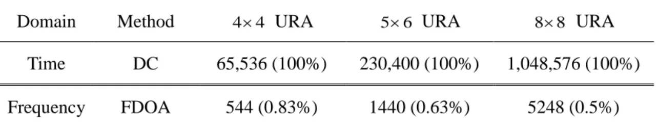
ABLES

Table 1. Comparison of computational complexity in terms of OPS of three

multichannels filtering methods for three array configurations. The block

size of FFT Ni 512_{. The numbers of microphones and focal points are}

assumed to be equal, i.e., m j . The DC method is used for benchmarking (100% in parenthesis). ... 31

Table 2. Experimentally Determined Relative Frequencies for a completely free square

VIII

L

IST OF

F

IGURES

Fig. 1. Top view of the experiment arrangement using a 5 6 URA. ... 33

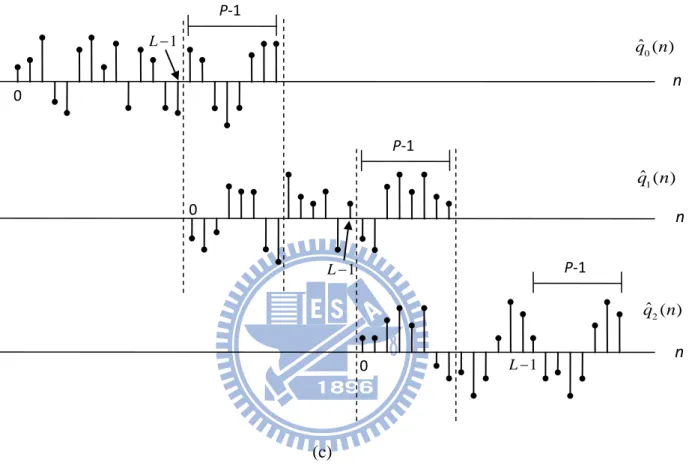
Fig. 2. Illustration of the Overlap and add method. (a) The pressure data p( )n , (b)

Decomposition of p n( )into non-overlapping sections of length L, (c) Result

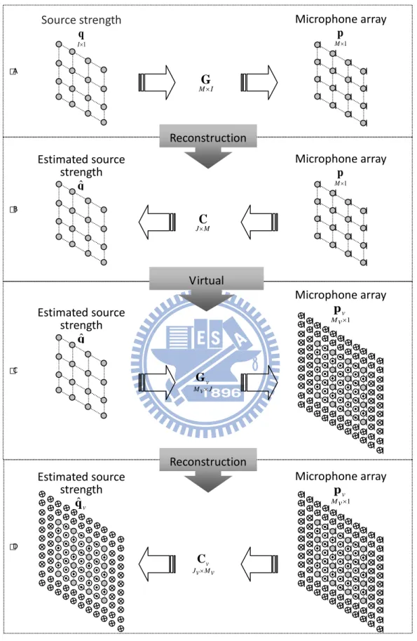
of convolving each section with the inverse filter ... 35 Fig. 3. The idea of the FDNESI with virtual microphone technique. The symbol“ ”

indicates an interpolated microphone position. The symbol“ ” indicates an

extrapolated microphone position. A The pressure data picked up by the

microphones, B Reconstructed source strength at the focal points, C The

pressure data interpolated at the virtual microphones, D Reconstructed source strength at the virtual focal points. ... 36

Fig. 4. The array settings for FDNESI using a 4 4 URA. ... 38

Fig. 5. The numerical simulation of NESI/FDNESI using the 4 4 URA and the

virtual microphone technique. (a) The unprocessed sound pressure image

received at the microphones, (b) the reconstructed active intensity image by

4 4 URA, (c) the reconstructed active intensity image using the virtual microphone technique in time domain processing, (d) the reconstructed active

intensity image using the virtual microphone technique in frequency domain processing. The symbol“ ” indicates the microphones. The symbol“”

indicates the focal points. The symbol“◇” indicates the noise sources. ... 42

Fig. 6. The numerical simulation result of vibrating plate by FDNESI using the

5 6 URA. (a) The reconstructed particle velocity with m=1, n=1 and f = 16.50 Hz, (b) the reconstructed particle velocity with m=2, n=1 and f = 33.57

IX

Hz, (c) the reconstructed particle velocity with m=2, n=2 and f = 65.98 Hz,

(d) the reconstructed particle velocity with m=3, n=2 and f = 97.45Hz. The

blue points are the microphones at the array surface and, black crosses are the

simulated point sources at the source surface and the black lines are the nodal lines. ... 46

Fig. 7. The numerical simulation of vibrating plate using the 5 6 URA and the virtual microphone technique. (a) The unprocessed sound pressure image

received at the microphones, (b) the real part of particle velocity in frequency

domain image, (c) the real part of particle velocity in frequency domain using

the virtual microphone technique image, (d) the nodal pattern with m=0,

n=2 and f = 48.78 Hz. The symbol“” indicates the microphones. The symbol“” indicates the virtual point sources. ... 50 Fig. 8. The experimental arrangement for a wooden box with a loudspeaker fitted

inside ,the URA, and a 30-channel random array optimized for farfield imaging are also shown in the picture. ... 51

Fig. 9. The results of run-up experiment obtained using FDNESI with the 4 4 URA. The scooter engine was accelerated from 1500 rpm to 7500 rpm within ten

seconds. (a) The unprocessed sound pressure image received at the

microphones, (b) the reconstructed active intensity image, (c) the

reconstructed active intensity image using the virtual microphone technique. The symbol“” indicates the focal points. ... 54 Fig. 10. The results of a wooden box with a loudspeaker fitted inside. The noise map is

within the band 200 Hz ~ 1.6k Hz. (a) The unprocessed sound pressure

image received at the microphones by 5 6 URA, (b) the particle velocity

X

indicates the focal points. ... 56

Fig. 11. The results of Loudspeaker experiment obtained using the 5 6 URA. The

loudspeakers are situated at (0.1m, 0.1m) and (0.4m, 0.2m) on the source

surface that produce random noise band-limited to 1.7 kHz. The observed

frequencies in the algorithms are chosen to be 1.2 kHz. (a) The reconstructed

sound pressure image by Fourier NAH, (b) the reconstructed sound pressure

image by FDNESI, (c) the source image obtained by using DAS, (d) the

source image obtained by using TR, (e) the source image obtained by using MVDR, (f) the source image obtained by using MUSIC. ... 62

Fig. 12. The results of compressor experiment obtained using the 5 6 URA. The

major noise is at the air intake position situated at (0.2m, 0.3m). The

observed frequencies in the algorithms are chosen to be 1.2 kHz. (a) The

reconstructed sound pressure image by Fourier NAH, (b) the reconstructed

sound pressure image by FDNESI, (c) the source image obtained by using

DAS, (d) the source image obtained by using TR, (e) the source image

obtained by using MVDR, (f) the source image obtained by using MUSIC. .. 68

Fig. 13. The experimental arrangement for a square aluminum plate driven from the

center with a shaker, the shaker is mounted on a desk. ... 69

Fig. 14. The results of vibrating plate experiment obtained using FDNESI with the

5 6 URA. (a) The real part of particle velocity in frequency domain image at 204Hz, (b) the real part of particle velocity in frequency domain image at

226Hz, (c) the real part of particle velocity in frequency domain image at

595Hz, (d) real part of particle velocity in frequency domain using the virtual

microphone technique image at 204Hz, (e) real part of particle velocity in

frequency domain using the virtual microphone technique image at 595Hz. The symbol“” indicates the focal points. ... 74

1

1. Introduction

Identification of noise source is the first step for diagnosing a noise problem and

also can be used in non-destructive evaluations. Much research about Noise source

identification (NSI) by sound field imaging using microphone arrays is raised [1-3].

NSI techniques can be divided into two parts: Nearfield Acoustical Holography (NAH)

[4] and Beamforming [5-6]. This paper is aimed at sound field visualization of the

algorithms, both the methods derived from NAH and the methods derived from

Beamforming in the nearfield. In 1980, the first paper dealing with NAH was

pioneered by Maynard and Williams [4]. While the traditional Fourier NAH method

provides a clear noise distribution, it has some limitations. The method requires the

source to be regular geometries such as planar surfaces and the placing of the

microphones need to be a regular grid of points. Microphone array must be larger than

the source area to minimize the windowing effect. The microphone spacing must be

less than one-half the wavelength to avoid spatial aliasing. However, most of these

limitations are result from the two-dimensional Fourier transform between the spatial

domain and the wave number domain. In a few years, many methods have been

developed to identify non-stationary noise [7] and reconstruct arbitrary shaped sources

[8-13]. In 2000, the Helmholtz Equation Least Squares (HELS) method represented

the sound field by using spherical wave was suggested by Wu [14]. A simple and

straightforward method, Equivalent Source Methods (ESM) was derived by direct

discretization of single-layer potential in the Helmholtz integral. The method has no

requirements regarding the source geometry and represented the sound field as a

distribution of discrete point sources [15-18]. Comprehensive coverage of NAH can

2

Recently, an NAH method termed the Nearfield Equivalent Source Imaging

(NESI) was introduced by the authors for noise source identification and sound field

reconstruction [21-23]. NESI is based on ESM concept and the main step is to design

the multichannel inverse filters. The multichannel inverse filters are designed offline

using truncated singular value decomposition (TSVD) or Tikhonov regularization. In

NESI, acoustical variables including sound pressure, particle velocity, and active can

be reconstructed. Without two-dimensional spatial Fourier transform, NESI avoid

many problems of Fourier NAH. NESI can also be implemented in the frequency

domain termed as FDNESI. With sparse microphones is available in applications, a

virtual microphone technique is used to improve imaging resolution and minimize edge

effects by interpolation and extrapolation. Another efficient frequency domain

processing technique, Frequency-Domain Overlap-Add (FDOA) is also introduced in

this paper. In addition to noise source identification, FDNESI are also used in

non-destructive evaluations such as mode shapes of plate vibration. The FDNESI are

validated by simulation and experiments and also compared with Fourier NAH by

experiments.

In addition to the methods derived from NAH, the methods derived from

beamforming and direction of arrival (DOA) estimation are also investigated in this

paper. The delay and sum algorithm (DAS) applies time shifts to the received signal to

compensate for the prorogation delays in the arrival of source signal at each

microphone [24-25]. A DOA estimation termed the time reversal (TR) algorithm is

based on a simple idea of reversing the received signal. For high resolution

beamforming methods, both the minimum variance distortionless response (MVDR)

algorithm and the multiple signal classification algorithm (MUSIC) employed a signal

covariance matrix. The MVDR algorithm finds the weight to improve resolution that

3

interference. The MUSIC algorithm used the eigenvalues and eigenvectors of a signal

covariance matrix to estimate the DOA of the signal received by microphone array

[24,26,27]. The methods derived from NAH and beamforming are compared by the

loudspeakers experiment and the compressor experiment.

2. Methods derived from NAH

2.1 Fourier NAH algorithm

In this section, the Fourier NAH is shortly reviewed. The 2D spatial Fourier

transform pair between the spatial domain and the wave number domain is show as:

( ) ( , , ) ( , , ) j k x k yx y x y p k k z   p x y z e  dxdy  

 

(1) ( ) 2 1 ( , , ) ( , , ) 4 x y j k x k y x y x y p x y z p k k z e dk dk    _{ }  

 

, (2)

where x, y and z are the Cartesian coordinates, dx and dy are the spacing of microphones

in the x and y directions, and kx and ky are the wave number components in the x and y

directions. In addition, the Wiener inverse filter is employed to mitigate the

ill-posedness during inverse reconstruction:

2 1 1 ( , ) ( , _{) 1 ( / ( , ) )} x y x y _{x y} W k k H k k _{ H k k}   , (3) where ( ) ( , ) jkz z zH x y H k k e 

, kz is the wave number in the z direction. In the k-domain,

the sound pressure of the reconstruction plane and the hologram plane can be related by

( ,_{x y}, ) ( ,_{x y}, _H) ( ,_{x y})

p k k z  p k k z W k k . (4)

4 particle velocity can be calculated by

( ,k k z_{x y}, ) p k k z( ,_{x y}, ) 

 k

u , (5)

where 2 f and k(k k k_x, _y, _z). The active intensity can be calculated by

1 Re{ } 2 p  Ι u . (6)

2.2 Frequency domain nearfield equivalence source imagine (FDNESI) algorithm

In this section, the proposed NESI algorithm [21] is shortly reviewed and presented in frequency domain (FDNESI) here. The vector q is the source strength on the source surface and the vector p is the pressure data picked up by the microphones can be related by the propagation matrix G as follows:

 p Gq, (7) where ₀ ( , , ) 4 sm jkr m s sm j e G r         G x y , (8) jkr e r 

is the free-space Green’s function [19] with rsm |xmys| being the distance

between the source point ys and the field point xm, where j 1, 0is the air density,

/

k c is the wave number,  _{is angular frequency, and c is the speed of sound.} In order to overcome the ill-conditioned from obtaining inverse filter, the problem

can be considered as a multiple-input-multiple-output (MIMO) model matching

problem: 2 min F  C W CG , (9) where 2

5

denotes the matching model into which frequency weighting and window functions can

be incorporated in addition to the simple identity matrix I. TSVD [28] or Tikhonov

regularization [29] is employed in the inverse filter design. The virtual source

strengths at the focal points are calculated by multiplication in frequency domain:

1 1 ˆ ( ) ( ) ( ) F M F M        q C p _{, (10)} ( )

F MC  denotes the inverse filter associated with the fth focal point and the mth

microphone, where the angular frequency 2 f , f is frequency in Hz. Hence, the obtained source strengths at the focal points serve as the basis for the subsequent

calculation of acoustical quantities including sound pressure, particle velocity and

intensity.

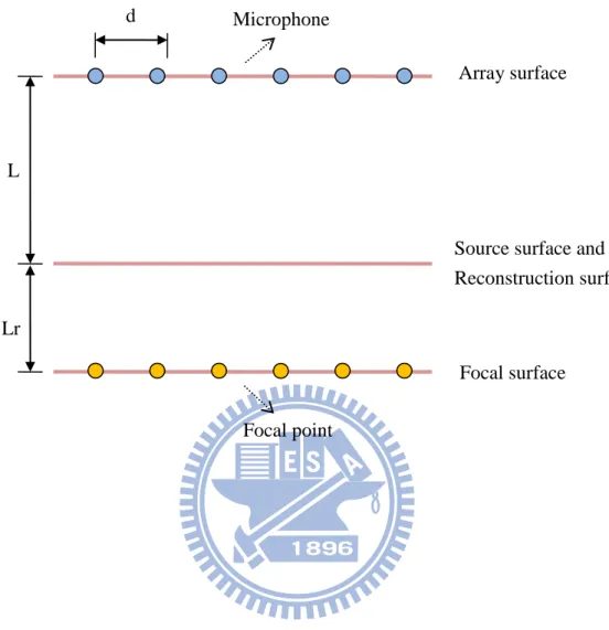
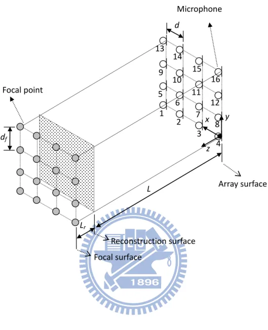
To avoid singularity, the focal points are retreated with a distance Lr = d/2 from the

reconstruction surface, as shown in Fig. 1. The sound pressure can be reconstructed as

ˆ ( ) ( ) ( ) r   r   p G q , (11) where 0 4 fr jkr r fr j e r      

G is propagation matrix associated with the fth focal point and

the rth reconstruction point and the normal particle velocity can be written as

0 0 0 ( , ) ( , ) ˆ( ) 4 ( ) 1 _{ˆ ( )} ( ) 4 fr fr n r jkr fr r fr jkr fr r fr fr j p j e d q r j j dr jkr _e r r       _                       x u x x n e q n e , (12)

where x vector is the reconstruction points, x vector is the focal points, ₀

0

( )

r   rfr

e x x , r_fr  x x₀ , k/c is wave number and ₀ is the density of air. The instantaneous normal active intensity is calculated by using

6



'



1 ( , ) Re ( , ) ( , ) 2 n r n I x   p x u x  . (13)

Root-mean-squares (rms) quantities can be calculated by time-averaging the

instantaneous squares quantities.

2.2.1 Frequency domain Overlap and Add method (FDOA)

Overlap-and-add technique can be used if continuous processing is desired. First,

partition the time-domain microphone pressure data

p( )

n

into non-overlapping

frames and zero-pad the frames into p ( )r n , where r = 1,2,…,R is the frame index and

R is the number of frames as shown in Figs.2(a) and (b). Transform each frame to the

frequency domain by using the FFT. Next, multiply the transformed pressure data

with the frequency-domain inverse matrix C( ) that can be computed offline. Finally, calculate the time-domain source amplitudes qˆ ( )_r n for each frame by using the inverse FFT and overlap and add the consecutive frames, as shown in Fig. 2(c).

To illustrate how to choose parameters in the overlap-and-add block processing,

consider the impulse response of the inverse filter matrix C( ) of length P. Assume that there are L samples in each framep_r( )n . Thus, the output of linear convolution

ˆ ( )_r n

q =C( )n *p_r( )n has the length (L+P-1). The linear convolution can be efficiently implemented, with the aid of FFT, by calculating the product C( ) pr( ) in the frequency domain, where N  L P-1 point FFT must be used to avoid

wraparound errors. To meet this length requirement, each frame must be padded with

(P-1) zeros. After inverse filtering, each frame of the source amplitude qˆ ( )_r n is added with (P-1) overlapped points. This is referred to as the

7

Frequency-Domain-Overlap-Add (FDOA) algorithm in the following presentation.

Tremendous computation efficiency can be gained because the frequency-domain

inverse matrix needs be computed offline for only once. The OPS of FDOA is

estimated to be

OPS(OA)(MJ) logN_i J M ₍₁₄₎ where M is the number of microphone, J is the number of focal points and Ni is

the block size.

2.2.2 Virtual microphone interpolation and extrapolation

In practical implementation of the FDNESI technique, an edge effect may occur

when the physical extent of source is larger than the patch array aperture. In addition,

the number of sensors may be too scarce to yield acceptable imaging resolution. To

address these problems, a virtual microphone technique is employed with field

interpolation (for improving resolution) and extrapolation (for reducing edge effect).

This following example demonstrates this technique using 4 4 uniform rectangular array (URA) with microphone spacing d. This rather coarse array configuration is to

be interpolated and extrapolated into 11 11 grid. The distance of reconstruction (DOR) is chosen to be d/ 2 so that the condition number of the propagation matrix

v

G was well below 1000 [21], where G is between the virtual microphone surface _v and reconstruction surface. In step C of Fig. 1, the source amplitudes on the focal

surface

1

ˆ

J

q estimated by FDNESI are used to calculate sound pressure p for a finer _v grid on the microphone surface:

1 ˆ ( ) ( , ) J j vj v v j vj q n p n r     



x (15)

8

where xv is the position vector of the field point on the microphone surface,

vj v j

r  x y , yj is the position vector of the jth point source on the focal surface, and

/

vj rvj c

  is the time delay. The sound pressures regenerated using Eq. (15) for the interpolated and extrapolated actual/virtual sensor locations with a finer spacing can be

assembled into the matrix form

1 1 ˆ ( ) ( ) ( ) v v J M_v M_v J n n n     p G q ₍₁₆₎ where v

G is the propagation matrix between the focal surface and the microphone surface, M_v   11 11 121 is the number of microphone and J   4 4 16 is the number of point sources on the focal surface. In the frequency domain, the sound

pressure is calculated by 1 1 1 ˆ ( ) ( ) ( ) ( ) ( ) ( ) v v v J M J M M_v M_v J M_v J               p G q G C p _{, (17)} where 1 1 ˆ ( ) ( ) ( ) J M J M       

q C p _{in Eq. (10). In Fig. 1, the interpolated and extrapolated}

microphones are indicated with the symbols “ ” and “ ”, respectively. Next,

choose a new point source distribution with finer spacing. The source amplitudes ˆq v

are estimated with the augmented inverse filters C in the frequency-domain as shown v

in step D of Fig. 1: 1 1 1 ˆ ( )_{v v} ( ) _v ( ) _v ( ) _v ( ) ( ) ( ) J M _M J_v J_v M_v M_v J_v M_v M_v J         _        q C p C G C p _{, (18)}

where M_v   11 11 121 is the number of virtual microphones and J_v   11 11 121 is the number of virtual point sources.

9

3. Methods derived from beamforming

3.1 Delay and Sum (DAS) algorithm

Considering an URA with the spacing d, the frequency is  and the speed of

sound is c. For M microphone signals x₁(t),,x_M(t), the data vector can be formed

as 1 1( ) 1( ) ( ) ( ) ( ) ( ) ( ) ( ) ( ) M M M x r j c j t x r j c x t n t t r r t t x t n t e s t e e                    _{ }_{ } _{ }                x a n , (19)

where a(r ) is called the array manifold vector, r t( )s t e( ) j t is the signal with frequency  at a reference point, s t( )is the phasor of r t( ) and n( )t is the noise vector. The output of DAS beamformer is defined as

0 1 ( , ) ( ) M m m m y t  x t   



 , (20)

where x t is the signal received by mth microphone, as shown in Eq. (19). In Eq. _m( ) (20), _m are the steering delays appropriate for focusing the array to the look direction,₀, and compensation for the direct path propagation delay associated with the desired signal at each microphone. The delay of each channel in Eq. (20) can be

calculated by m m x c    , (21)

where x_m is the distance between reference source positions _s and mth microphone. However, the delay usually is not an integer number in the digital signal

10

processing. Lagrange interpolation is employed to deal with the fractional delay

problem [30].

3.2 Time Reversal (TR) algorithm

The Time Reversal (TR) algorithm is based on an idea of reversing the received signal. The sound pressure data p( )t is recorded by a microphone array, time-reversed and then re-transmitted into the medium. The re-transmitted signal p(Tt) propagates back through the same medium and refocuses on the source where T is the

delay due to causality requirements which is decided by sampling time.

3.3 Minimum Variance Distortionless Response (MVDR) algorithm

Another approach has been proposed using the data covariance matrix. This

method has been shown to provide higher resolution in DOA estimations than the DAS

algorithm. In order to facilitate digital processing, we simultaneously sample all array

inputs to form digital data x t_m( )x kT_m( ), k 1, 2, . For D sources, we may invoke the principle of superposition to write

1 1 1 ( ) ( ) ( , ) ( ) ( ) [ ( , ) ( , )] ( ) ( ) ( ) ( ) D i j i i j r k k r k k k r k k k               _{ }      



x a n a a n Ar n , (22)

where _i is the direction of the ith source, r(k) is the source signal vector and A is DOA matrix. A beamformer output is a linear combiner that produces an output signal

11 1 ( ) ( ) ( ) M H m m m y k w x k k  



w x , (23)

where w is the weight vector given by [ ₁ ]T M

w w



w . Because the MVDR method exploits the correlation between array input signals, it is necessary to calculate the array

signal correlation matrix.



( ) H( )



xx E k k

R x x , (24)

Suppose that the noise is uncorrelated with signals E



r( )k nH( )k



0 and the noise is spatially white E



n( )k nH( )k



_n2I . By the preceding assumption, the Eq. (24) can be rewritten as



 



2 ( ) H( ) ( ) H( ) xx H rr nn H rr n E k k E k k        R A r r n n AR A R AR A I , (25)

where Rrr and Rnn are the source and noise correlation matrices, respectively. In

practice, the data correlation matrix Rxx is usually approximated by the data covariance

matrix:

( ) H (1 ) ( 1), 1, 2 , (0)

xx p  p p  xx p p P xx 

R x x R R 0. (26)

At this recursive equation,  is a constant which satisfied 0  1. The received signal is divided to p frames and rearranged to the data vector x[ x x_{1 2} xp].

In the following, the aim is to find the MVDR weight vector w_MV . An optimization problem is given for solving the unknown vector w_MV. The MVDR beamformer attempts to minimize the output power



2





2



( ) HMV ( ) MVH xx MV

E y k E w x k w R w . (27)

12

MVDR beamforming suppresses the undesired interference and the noise from   ₀. The problem can be expressed as follows

0 min subject to ( , ) 1 MV H MV xx MV MV       w w R w w a , (28)

This problem can be solved by Lagrange multiplier method

0 0 [ ( , ) 1] 0 ( , ) 1 MV MV H MV xx MV MV MV               w w R w w w a w a , (29)

After calculations, the MVDR weight can be obtained as:

1 0 1 0 0 ( , ) ( , ) ( , ) xx MV H xx          R a w a R a , (30)

The spatial power spectrum S_MV( ) exhibits D peaks approximately at ₁ _Dis show as: 1 1 ( ) ( , ) ( , ) H MV MV xx MV H xx S       w R w  a R a . (31)

3.4 Multiple Signal Classification (MUSIC) algorithm

In contrast to MVDR which is based on the covariance matrix of the received

signals, an approach of DOA estimation has been proposed by exploiting the eigenvalue

decomposition (EVD) of the covariance matrix. The array covariance matrix Rxx is

represented by EVD: 2 1 H xx rr n     R AR A I UΛU , (32)

where U is a unitary matrix and comprise M linearly independent eigenvectors

1 M

u u . The eigenvector associate with M eigenvalues ₁ _M . The array correlation matrix can be represented as

13 1 1 1 2 2 1 2 1 0 0 0 0 [ ] 0 0 H xx H H M H M m m m m H M M                      _{ }            



R UΛU UΛU u u u u u u u u . (33)

The diagonal terms of Λ have been arranged with  ₁ ₂  _M. The noise term

2 n  I can be yielded to 2 2 1 2 2 1 M H H n n n n m m m         



I UU UU u u . (34)

Because A consists of D sources, we assume that A and Rrr are of full rank D.

Subsequently the signal-only correlation matrix Cxx is generated by subtracting the

noise component from Rxx

2 1 ( ) M H H x x rr m n m m m     



 C AR A u u . (35)

If Rrr is rank D and small than the array size M, the smallest M D eigenvalues

1

D M

 _  are equivalent to the noise power. Therefore the range of Cxx are spanned

by u to ₁ u . If the array has no coherent source between any of two received signals, _D Rrr only has nonzero values on the diagonal terms which represents the power of the D

sources. Note that the range of Cxx is identical to the range of A which is spanned by

the manifold vectors a( , ) ₁ a( , _D). The relation between Cxx and A is

 

span



( , 1), , ( , D)



span



1, , D



R A  a   a    u u (36)

and

 

span



D 1, , M



R A   u _ u , (37)

where span



u₁, ,u_D



and span



u_D₁, ,u_M



are called the source subspace and noise subspace, respectively. Because the source subspace is orthogonal to the noise

14 subspace such that

( , ) 0, 1, 2, , ; 1, 2, ,

s

H

m  d  ds  D m D D M

u a . (38)

The MUSIC technique is to exploit Eq. (38) to improve the DOA estimations. The

eigenvectors u_D1, ,u is used to construct the projection matrix as follows _M

1 M H m m N m J  



u u P . (39)

From Eq. (34), the direction of the source _i (i1, , )D can be found by solving

1 ( , ) ( , ) , s M H N m m d m J         



  P a u u a 0 . (40)

The projection matrix has the properties of 2 H N  N and N  N

P P P P . The problem of Eq. (40) can be extended to solve Eq. (41) for simplicity.

2 2

( , ) ( , )H H ( , ) 0,

N      N N      i

P a a P P a . (41)

Equivalently, the inverse of Eq. (41) has the infinitely value when   _i, i1, ,D. The inverse of Eq. (41) is denoted as MUSIC spectrum.

1 ( ) ( , ) ( , ) MU H N S       a P a . (42)

15

4. Numerical simulations

4.1 Virtual microphone interpolation and extrapolation

A URA with M   J 4 4 is employed in this simulation, as depicted in Fig. 4.

The spacing of the microphones (d) and the focus points (d_f) were both selected to be 0.1m = λ / 2 for 1.7 kHz. Another important parameter to choose is distance of

reconstruction (DOR) that entirely depends on the degree of ill-posedness of the

inverse problem. Assume that the acoustic radiation problem can be formulated via

ESM into the following matrix equation

Ax = b, (43) where b and x are the hologram data and source data, respectively, which are related by

the propagation matrix A. It can be shown the perturbation term b of the data vector such as measurement noise, numerical error, etc., and the perturbation term x of the reconstructed data satisfy the following inequality [31]

cond( )    x b A x b , (44) where cond( )A _max/_min is the condition number of the matrix A and symbolizes vector 2-norm. Therefore, as an indicator of the ill-posedness inherent in

the inverse filtering process, the condition number can also be regarded as a

magnification factor of perturbations as well as loss of SNR after inverse filtering. For

example, the SNR of data will be reduced by 60 dB of dynamic range after inverse filtering if cond( ) 1000A  . It is well known that condition number of the propagation matrix increases with the DOR since the evanescent wave decays rapidly with the

16

DOR. Thus, given a 60 dB tolerance of loss of SNR, a DOR that gives a condition

number less than 1000 is generally deemed appropriate. In the following examples, DOR ( )L was chosen to be d/ 2 to yield a condition number less than 1000.

In the inverse filter design, Tikhonov regularization parameter was selected

according to the L-Curve method [32]. The OPS required by DC and FDOA is

compared for three different array configurations (16, 30 and 64 channels) in Table 1.

The number of FFT frequency points Ni = 512. The numbers of microphones and focal

points are assumed to be equal, i.e., M J. The most computationally expensive DC

method is used for benchmarking as 100% (in parenthesis) OPS requirement. It is

obvious from the comparison that the computation efficiency is considerably improved

using the FDOA approach, especially for large number of microphone channels (only

5% of the benchmark DC method for a 64-channel array).

In the example, three random noise sources (band-limited to 1.7 kHz) are situated

at (0m, 0m), (0.6m, 0.6m) and (1.2m, 1.2m), respectively. Specifically, two sources

are situated at the kitty corners and the remaining source is situated at the center on the

focal surface. Figure 5 (a) shows the unprocessed sound pressure (rms) in linear scale

received at the microphones. From the quite blurred image, three noise sources were

barely resolvable, particularly for the noise source at the center. Figure 5(b) shows the

sound intensity (rms) calculated by the time-domain NESI. Although the image

quality is slightly improved, the noise source at the center (0.6m, 0.6m) is still not

identifiable because it is not located on the focal point. To overcome this problem,

virtual microphone technique was applied to interpolate and extrapolate the pressure

field on the microphone surface and increase the number of microphones and focal

points from 4 4 to 11 11 . In total, 33 and 72 microphones are uniformly distributed inside (interpolation) and outside (extrapolation), respectively, the original

17

time-domain NESI is shown in Fig. 5(c). It can be clearly observed from the result that

the quality of the reconstructed image was significantly improved. Problems due to

edge effect and insufficient resolution were basically eliminated. Three sources

including the one at the center are clearly visible in the intensity map. Total sound

power level is 148.8 dB re. 12

1 10  W. This array setting will be used in the following scooter experiment.

In addition to the simulation above, the frequency-domain NESI is used to identify

random noise sources with the same setting as in the time-domain NESI. Here, 512

point FFT with Hamming window is employed in the simulation. Figure 5(d) shows

the active intensity (rms) calculated by the frequency-domain NESI. Although three

sources are well located in Fig. 5(d), they exhibit slightly larger spreading than the

result in Fig. 5(c) obtained using the time-domain NESI.

4.2 Vibrations of plates

In addition to noise source identification, FDNESI can also be used in

non-destructive evaluations. Numerical simulation is conducted to validate the

FDNESI on detecting the mode shapes of vibrating plate.

4.2.1 Rectangular plate with SS-SS-SS-SS boundary condition

An acrylic fabric rectangular plate with 0.36m long, 0.26 wide and 0.001m thick

was used to simulation. The aperture of the plate and the 5 6 URA are the same with the microphone spacing dx = 0.072m, dy= 0.065m in x and y directions. The

18

is L_r = L/ 2 = 0.0325m. The boundary conditions of the plate are assumed as all sides simply supported (SS):

0, 0 ( 0, ) 0, 0 ( 0, ) x y w M for x a w M for y b          , (45)

where w is the deflection, M and _x M_y are the moments in the x and y directions, respectively , a is the plate length of long side and b is the plate length of wide side.

The mode shape (deflection function) of rectangular plate is defined as [33]:

sin sin sin

mn mn m x n y W A t a b   _   , (46)

where A is an amplitude coefficient determined from the initial conditions, _mn m and

n are the number of nodal lines lying in the x and y directions, is the angular frequency and t is time. The resonance frequency of the rectangular plate is:

2 2 A D m n a b     _{   }   _{ } _{ }         . (47) where





3 2 12 1 Eh D  

 is the flexural rigidity, E is Young’s modulus, h is the plate thickness,  is Poisson’s ratio, _A is mass density per unit area. The sound pressure can be obtained by Rayleigh integral:

0 ( ) 2 sm jkr sm A ck e P j u dA r    



x . (48)

where ₀is the air density, c is the speed of sound, k/c is the wave number, uis velocity, j 1_, r_sm |x_my_s | being the distance between the source point ys and the field point xm and A is the area of the plate. Substituting Eq. (46) into Eq. (48)

becomes 0 1 ( ) ( ) 2 sm mn S sm r P W t r c    



  x . (49)

19

where s is the number of source points. The delay problem is figure out by Lagrange

interpolation [30].

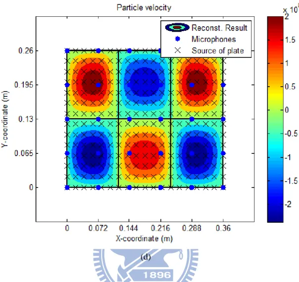
For an acrylic fabric rectangular plate, parameters are setting as follows: E =

3.03x109 Pa, a= 0.36m, b= 0.26m, h= 0.001m,  = 0.3,  = 1190 kg/m3, _A=

h= 1.19 kg/m2, ₀=1.21, c=343 m/s and the sampling rate is 1 kHz. After the

processing of FDNESI, the real part of particle velocity in frequency domain is shown in Fig. 6(a)-(d). With m=1, n=1 and f = 16.50 Hz (2 f ), the plate have a great amplitude at the center as shown in Fig. 6(a). From Fig. 6(b), the plate have two

peaks at the center of left half plate and right half plate which are out of phase, parameters setting are m=2, n=1 and f = 33.57 Hz. In higher order mode shapes,

the result are shown in Fig. 6(c)(d) with (1) m=2, n=2 and f = 65.98 Hz , (2) m=3,

n=2 and f = 97.45Hz, the noise source distribution are symmetry and have regular

phase difference.

4.2.2 Square plate with F-F-F-F boundary condition

An aluminum plate with 0.2m side length and 0.002m thick was used to simulation.

The aperture of the plate and the 5 6 URA are the same with the microphone spacing dx = 0.04m, dy = 0.05m in x and y directions. The distance between source surface and array surface L = 0.02m and the retreat distance is L_r= L/ 2 = 0.01m. The boundary conditions of the plate are assumed as all sides free (F). The mode

shape (deflection function) of square plate is defined as [33]:

cos cos cos cos sin

mn mn m x n y n x m y W A t a a a a     _    _  _   , (50)

20

plate length, m and n are the number of nodal lines lying in the x and y

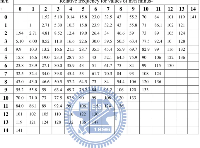
directions, is the angular frequency and t is time. The resonance frequencies of the square plate can be found in Table 2 by [34], the ratios of frequencies relative to

the fundamental are given for various m n ratios and the fundamental frequency of / the plate we use is 25.1465 Hz [34]. The sound pressure can be obtained by Rayleigh

integral by eq. (49) as mentioned before. For an aluminum square plate, parameters are setting as a= 0.2m and the sampling rate is 0.5 kHz. With m=0, n=2 and f =

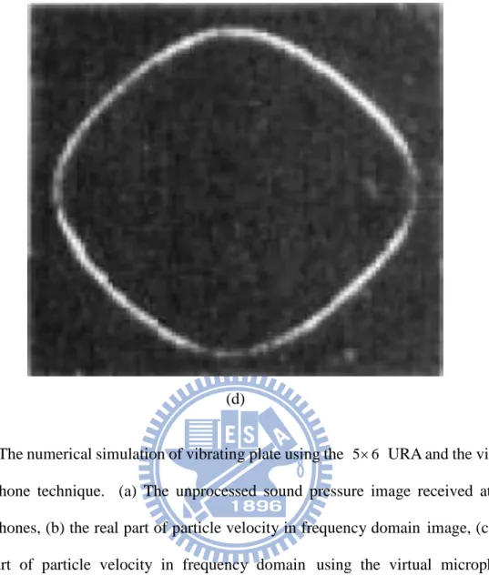
48.78 Hz (2 f ), the results are shown in Fig. 7(a)-(c). The received signal by microphone array is shown as Fig. 7(a). After the processing of FDNESI, Fig. 7(b)

shows the real part of particle velocity in frequency domain. For getting good

resolution, interpolation of virtual microphone is applied in FDNESI and the result is

shown as Fig. 7(c). The theoretical nodal pattern is shown as Fig. 7(d) [34]. From

above, the identification of vibrating plate mode shape by FDNESI is effective and is

21

5. Experimental verifications

5.1 Experimental Arrangement (1)

To validate the FDNESI technique, practical sources including a scooter and a

wooden box model with a loudspeaker fitted inside were chosen as the test targets for

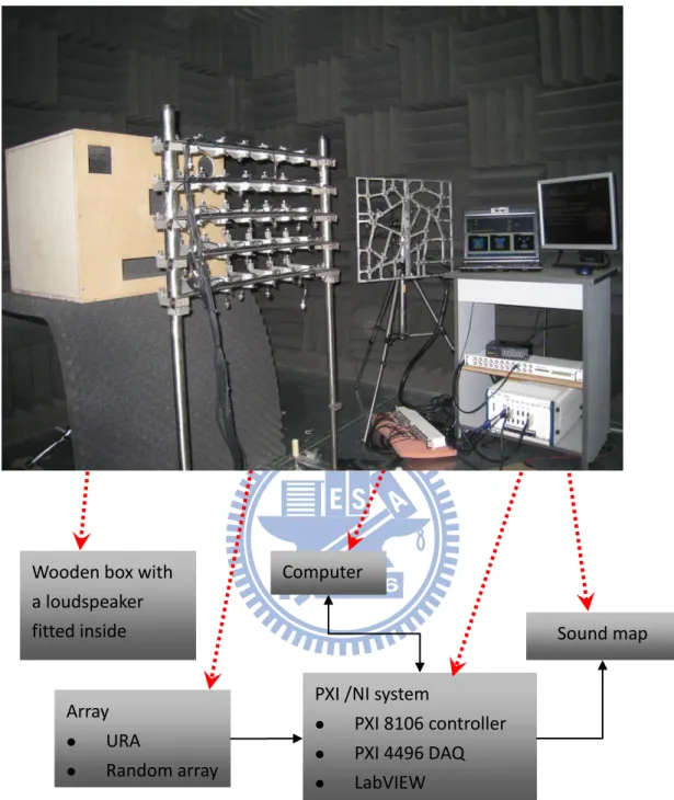
experiments. Figure 8 shows the block diagram of the experimental arrangement. In

the scooter experiment, the array configuration is a 4 4 URA, while in the wooden box experiment, the array configuration is a 5 6 URA. Two PXI 4496 systems [35]

in conjunction with LabVIEW [35]were used for data acquisition and processing at the

sampling rate 5 kHz. A bandpass filter (20 Hz~1.7 kHz) is used to prevent aliasing and

errors occurring in the out-of-band frequencies. The source amplitude, sound pressure,

particle velocity and sound intensity reconstructed using FDNESI can be displayed on

the monitor.

5.2 Scooter Experiment

In the experiment, a 125cc scooter served as a practical source to examine the

capability of FDNESI in dealing with non-stationary sources. The scooter is mounted

on a dynamometer inside a semi-anechoic room. The array parameters are selected to

be M = J = 4 4 , d = df = 0.1m = λ/2 for 1.7 kHz and L = d/ 2 . The Frequency-domain FDNESI was used to reconstruct the sound field on the right side of

the scooter in a run-up test. The engine speed increased from 1500 rpm to 7500 rpm

within ten seconds. The unprocessed sound pressure received at the microphones is

22

Fig. 9(b). These results revealed that the cooling fan behind the vented engine cover

was the major noise source. Next, the virtual microphone technique is employed to

see if it is possible to further enhance the image quality by increasing the number of

channels from 4 4 16 to 11 11 121  . The inverse filters have been designed in the previous numerical investigation. The particle velocity was then reconstructed on

the basis of the estimated source amplitude, as shown in Fig. 9(c). Total sound power

level is 195 dB re. 1 10 12W. Clearly visible is a larger area of image with improved resolution than that of Fig. 9(b), where again the cooling fan is the major noise source.

5.3 Wooden Box Experiment

In this experiment, a wooden box model with loudspeaker fitted inside is used to

validate the FDNESI technique by using a 5 6 URA. As shown in Fig. 10(a),

several holes with different shapes are cut in the front face of the box like a

Jack_O_Lantern. A circle, two squares, and a slit are located at (0.5m, 0.4m), (0m,

0.4m), (0.25m, 0.25m) and (0.25m, 0m), respectively. The loudspeaker produces

random noise band-limited to 1.7 kHz. The microphone spacing d is selected to be

0.1m (λ/2 corresponding to f_max= 1.7 kHz).

Figure 10(a) shows the unprocessed sound pressure picked up at the microphones

within the band 200 ~ 1600 Hz. From the image, the noise sources were barely

resolvable, particularly for the noise source at the edge - the circle, the slot and the

square at upper left corner. Also, the square at the center was difficult to distinguish.

Virtual microphone technique was again applied to overcome this problem by

interpolate and extrapolate the pressure field on the microphone surface and increase

23

setting, the particle velocity (rms) reconstructed using the frequency-domain FDNESI

is shown in Fig. 10(b). It can be clearly observed from the result that the quality of the

reconstructed image was significantly improved. Problems due to edge effect and

insufficient resolution were basically eliminated. The FDNESI images apparently

yielded more reliable information about noise sources than the unprocessed sound

pressure.

5.4 Experimental Arrangement (2)

To compare the algorithms as mentioned in this paper, practical sources

including loudspeakers and a compressor were chosen as the test targets for

experiments. The experiments were undertaken in a semi-anechoic room. The microphone array configuration is a 5 6 URA with spacing dx = dy= 0.1m (λ/2

corresponding to f_max= 1.7 kHz) in the x and y directions and the distance between

source surface and array surface L=0.1m. Two PXI 4496 systems [35] in conjunction

with LabVIEW software [35] were used for data acquisition and processing at the

sampling rate 5 kHz. A bandpass filter (20 Hz~1.7 kHz) is used to prevent aliasing and

errors occurring in the out-of-band frequencies.

5.5 Loudspeaker experiment

In this experiment, two loudspeakers are used to validate the Fourier NAH, FDNESI, DAS, TR, MVDR and MUSIC algorithms in the nearfield with comparison.

The loudspeakers are situated at (0.1m, 0.1m) and (0.4m, 0.2m) on the source surface

that produce random noise band-limited to 1.7 kHz. The observed frequencies in all

24

six acoustic imagine algorithms with 5 6 URA are shown in Fig. 11(a)-(f). From

the reconstructed sound pressure of Fourier NAH and FDNESI in Fig. 11(a)(b),

Fourier NAH can find out the two sources roughly while FDNESI have clearer source

distribution than Fourier NAH. From Fig. 11(c)(d), DAS have a poor result that is

unable to distinguish the two sources and TR can localize the two source positions but

with big main lobes. In high resolution MVDR and MUSIC algorithms, they can

localize the two sources precisely and the performance of MUSIC is better than

MVDR as shown in Fig. 11(e)(f).

5.6 Compressor experiment

In the experiment, a compressor served as a practical source to examine the

capability of the six algorithms. The compressor is mounted on a table inside a

semi-anechoic room that the major noise is at the air intake position on the top of the

compressor and the minor noise is low intensity vibration at overall body. Different

with loudspeaker experiment, the source of this experiment is not on the planar

surface. The observed frequencies in the algorithms are chosen to be 1.2 kHz. The

noise images obtained by processing of the six algorithms with URA are shown in Fig.

12(a)-(f). From Fig. 12(a), Fourier NAH has a terrible noise source distribution,

consistent with the theory that the source should be planar in Fourier NAH to identify

successfully. From the reconstructed sound pressure of FDNESI shown in Fig. 12(b),

FDNESI can identify the major source at the air intake and the vibration at overall

body. The result of DAS is bad by wrong location and very big main lobe but TR

provide an acceptable result as shown in Fig. 12(c)(d). In the noise images of

MVDR and MUSIC, they identified the noise source at the air intake accurately and

25 5.7 Vibrations of free square plate experiment

The experiment is conducted to validate the FDNESI on detecting the mode

shapes of vibrating plate. An aluminum plate with 0.2m side length and 0.002m thick

was used to in the experiment. The aperture of the plate and the 5 6 URA are the same with the microphone spacing dx = 0.04m, dy= 0.05m in x and y directions.

The distance between source surface and array surface L = 0.02m and the retreat distance is L_r= L/ 2 = 0.01m. The edges of the plate were unbounded and the plate

was excited by a shaker from its center using a random noise signal. The experiment

was undertaken in a semi anechoic room and the experimental arrangement is shown

in Figure 13. In order to confirm the experimental result, the salt is sprinkled on the

vibrating plate for visualize the nodal lines, the salt is thrown off the moving regions

and piles up at the nodes. The frequencies were chose by the peaks of the microphone’s frequency response. By exciting the plate at the frequencies we chose,

we can find three mode shapes at 204 Hz, 226 Hz and 595 Hz, the real part of particle

velocity in frequency domain after the processing of FDNESI are shown in Fig.

14(a)-(c). For getting better resolution of the results, interpolation of virtual

microphone is applied in FDNESI at the frequencies of 204 Hz and 595 Hz that the

result is shown as Fig. 14(d)(e). From the Fig. 14(a)(d), we can obtained a consistent

result with simulation. From the experimental results that we can conclude the

26

6. Conclusion

Various implementation issues of the FDNESI technique have been investigated

in this paper. A virtual microphone technique is suggested for minimizing edge

effects using extrapolation and for improving resolution using interpolation.

Although the FDNESI is by far the most efficient method among all inverse filtering

approaches, it can yield a noise source mapping with slightly larger spreading than the

NESI. The FDNESI technique proved effective in identifying broadband and

non-stationary sources produced by these sources.

Sound field imaging using microphone array by FDNESI algorithm are capable

to reconstruct the sound field effectively which is suggested in the thesis by noise

source identification and non-destructive mode shape evaluations. From the

loudspeaker experiment and the compressor experiment, the six algorithms are

compared on the point of resolution and performance. Both Fourier NAH and

FDNESI have good performance while FDNESI is more robust than Fourier NAH for it

can reconstruct the sound field from the source of arbitrary shape. As expected, the

high resolution methods such as MVDR and MUSIC can obtain greater results than

DAS and TR in localizing the source position. Although the resolution of MVDR and

MUSIC are better than Fourier NAH and FDNESI but the performance of Fourier

NAH and FDNESI are better. Most important of all, Fourier NAH and FDNESI can

reconstruct the acoustic variables such as sound pressure, particle velocity and active

27

References

[1] V. Murino, Reconstruction and segmentation of underwater acoustic images

combining confidence information in MRF models, Journal of the Pattern

Recognition Society 34 (2001) 981-997.

[2] Y. Fan, B. Tysoe, J. Sim, K. Mirkhani, A. N. Sinclair, F. Honarvar, H. Sildva, A.

Szecket, R. Hardwick, Nondestructive evaluation of explosively welded clad rods

by resonance acoustic spectroscopy, Ultrasonics 41 (2003) 369-375.

[3] U. Benko, J. Petrovcic, D. Juricic, J. Tavcar, J. Rejec, A. Stefanovska, Fault

diagnosis of a vacuum cleaner motor by means of sound analysis, Journal of Sound

and Vibration 276 (2004) 781–806.

[4] E. G. Williams and J.D. Maynard, Holographic imaging without the wavelength

limit, Physical Review Letters 45 (1980) 554-557.

[5] B. D. V. Veen, K. M. Buckley, Beamforming: a versatile approach to spatial filtering,

IEEE ASSP Magazine (1998) 4-24.

[6] H. Krim, M. Viberg, Two decades of array signal processing research, IEEE Signal

Processing Magazine (1996) 67-94.

[7] J. Hald, Non-stationary STSF, Brüel & Kjæ r Technical Review No. 1, 2000.

[8] W.A. Veronesi, J.D. Maynard, Digital holographic reconstruction of sources with

arbitrarily shaped surface, Journal of the Acoustical Society of America 85 (1988)

588–598.

[9] M. R. Bai, Application of BEM (boundary element method)-based acoustic

holography to radiation analysis of sound sources with arbitrarily shaped

geometries, Journal of the Acoustical Society of America 92 (1992) 533-549.

28

enclosing an interior space using the boundary element method, Journal of the

Acoustical Society of America 100 (1996) 3030–3016.

[11] S. C. Kang, J. G. Ih, Use of non-singular boundary integral formulation for

reducing errors due to near-field measurements in the boundary element method

based near-field acoustic holography, Journal of the Acoustical Society of

America 109 (2001) 1320-1328.

[12] N. P. Valdivia, E. G. Williams, J. Klos, Reconstruction of the acoustic field using a

conformal array, Proceedings of Inter-noise (2006)

[13] J. Hald, J. Gomes, A comparison of two patch nah methods, Proceedings of

Inter-noise (2006)

[14] S. F. Wu, On reconstruction of acoustic pressure fields using the Helmholtz

equation least squares method, Journal of the Acoustical Society of America 107

(2000) 2511-2522.

[15] A. Sarkissian, Method of superposition applied to patch near-field acoustical

holography, Journal of the Acoustical Society of America 118 (2005) 671-678.

[16] J. Gomes, J. Hald, P. Juhl, F. Jacobsen, On the applicability of the spherical wave

expansion with a single origin for near-field acoustical holography, Journal of the

Acoustical Society of America 125 (2009) 1529-1537.

[17] P.A. Nelson, S.H. Yoon, Estimation of acoustic source strength by inverse

methods: part I, conditioning of the inverse problem, Journal of Sound and

Vibration 233 (2000) 643–668.

[18] P. A. Nelson, S. H. Yoon, Estimation of acoustic source strength by inverse

methods: part II, experimental investigation of methods for choosing

regularization parameters, Journal of Sound and Vibration 233 (2000) 669-705.

[19] E.G. Williams, Fourier Acoustics, Academic Press, New York, 1999.