A New Parallel Reconfigurable Computing
Archi-tecture and Hidden Markov Model Application
Yung-Chuan Jiang, Anand Paul, Jhing-Fa Wang Department of Electrical Engineering,
National Cheng Kung University [email protected]
Abstract―Parallel processing techniques are
increas-ingly found in reconfigurable computing, especially in digital signal processing (DSP) applications. In this paper, we design a parallel reconfigurable computing (PRC) ar-chitecture which consists of multiple dynamically recon-figurable computing (DRC) units. The hidden Markov model (HMM) algorithm is mapped onto the PRC archi-tecture. First, we construct a directed acyclic graph (DAG) to represent the HMM algorithms. A novel parallel parti-tion approach is then proposed to map the HMM DAG onto the multiple DRC units in a PRC system. This parti-tioning algorithm is capable of design optimization of parallel processing reconfigurable systems for a given number of processing elements in different HHM states.
Index Terms―FPGA, parallel processors,
reconfigur-able processing, HMM, partitioning algorithm.
I. INTRODUCTION
Reconfigurable computing (RC) is a promising alternative to application-specific integrated cir-cuits (ASIC) and general-purpose processor sys-tems, providing software processor flexibility, hardware coprocessor efficiency, high throughput and enhanced speed. Field programmable gate ar-rays (FPGAs) are the most common devices used for RC, but “on-the-fly” dynamic reconfiguration has emerged as an attractive technique for mini-mizing reconfiguration time. In particular, dynami-cally reconfigurable computing (DRC) [1] [2] is receiving growing interest because its utilization of computational logic units can be dramatically im-proved by logical time-sharing. On-chip resources can be reused, cutting hardware costs and improv-ing performance. Therefore, this paper utilizes dy-namically reconfigurable computing architecture to implement the HMM algorithm. Massive parallel-ism, a special focus of this present paper, is
consid-ered a strong contender improved DSP chip designs. Moreover, the inherent parallelism in the HMM algorithm motivates us to propose a parallel proc-essing architecture for its implementation.
The parallel processing technique is generally used in a multiple instruction, multiple data (MIMD) architecture [5] to help optimize system performance. MIMD organization with multiple processors and I/O processors access one or more memory modules via a bus. Traditional non-dynamic RC architecture may be considered as multiple processor elements (PEs) sharing a single physical memory. A control processor executes the RC units, accessing memory through a shared memory bus. However, the MIMD architecture has the following drawback. Because all memory ref-erences pass through the common bus, there is a data bottleneck at this bus.
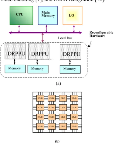
To reduce bus access numbers, equipping each processor with its own local memory as a dynami-cally reconfigurable computing machine with sev-eral configurations is desirable. The following dis-cussion will assume the availability of such hard-ware. Prior studies have shown that architecture consisting of several parallel non-dynamic RC units implemented as parallel FPGA can improve system performance [7]-[8]. In consequence, this present paper extends the above ideas by presenting a par-allel reconfigurable computing (PRC) machine which combines several parallel FPGA arranged as parallel dynamically reconfigurable computing machines. In the PRC architecture, the proposed DRC-based processors are directly and easily us-able in a symmetric multi-processor organization [5]. Figure 1(a) shows the proposed PRC
architec-ture. A set of individual dynamically reconfigurable parallel processing units (DRPPU), each imple-mented on its own FPGA, are connected in parallel by a common bus. Each DRPPU has its own local memory. Each DRPPU is composed of an array of configurable logic blocks (CLB), as seen in Figure 1(b). Such architecture maximizes potential system performance for high computation and data inten-sive applications [9]-[11] such as MPEG-4, H.264 video encoding [7], and HMM recognition [12].
(a)
(b)
Figure 1. (a) Parallel reconfigurable computing architecture: each DRPPU has a local memory. (b) DRPPU architecture.
In a PRC system, the DRPPU is a dynamically reconfigurable computing processor similar to the fine grained architecture of DRFPGA [6]. DRC units have been used to realize large systems using multiple configurations [3]-[4]. Importantly for PRC implementation, the HMM algorithm can be partitioned into multiple stages and stored in con-figuration memory planes. In general, DRC units hold only one active configuration in any time frame. Each configuration is called a cycle. All combinational logic is evaluated and flip-flop val-ues are updated in one cycle. [6]. Each CLB has microregisters that store intermediate values
gener-ated from combinational logic for later cycle use and also hold flip-flop values for next cycle use. A cycle begins by saving all previous cycle CLB re-sults in microregisters and then a new configuration is loaded into the active configuration of the local memory.
The remainder of this paper is organized as fol-lows. Section II introduces the HMM algorithm and uses data flow graphs (DFG) to represent it. Sec-tion III presents the problem formulaSec-tion. SecSec-tion IV proposes parallel partitioning for mapping HMM DAG onto a PRC system. Experimental re-sults are presented in Section V. Finally, conclu-sions are given in Section VI.
II. HIDDEN MARKOV MODEL AND CORRESPONDING
DATA FLOW GRAPH
A. Hidden Markov Model
The Hidden Markov model is a class of statisti-cal models useful for analyzing a discrete time se-ries of observations such as a stream of acoustic elements extracted from a speech signal. An HMM is characterized by the state transition probability distribution, observation probability distribution and initial state probability distribution. For an HMM consisting of N states S1, S2, …., SN, we
de-note the state transition probability distribution as A = { aij }, where aij is the state transition probability
from state Si to state Sj. The observation probability
distribution is represented by B = {bj(ot)}, where
bj(ot) is the probability of having an observation
vector o(t) at time-step t being in the state j. The initial state probability distribution is represented by = {j}, where j is the initial probability in the
j-th state. The above three distributions can be
in-dicated compactly by λ= (A, B, ). For an
observa-tion sequence O = [o1, o2,…, oT], the recognition
result relies on HMM probability evaluation, i.e. calculating the observation sequence probability
P(O|λ). In our VLSI design, we focus on the
recog-nition capability of the HMM. The HMM parame-ter λ is assumed to be computed in advance and stored in the memory unit. The HMM algorithm in this paper performs the HMM probability evalua-tion process.
While the conventional HMM evaluation process computes P(O|λ) using the forward-backward
algo-CPU Main Memory
Local bus I/O Reconfigurable Hardware . . . Memory DRPPU DRPPU DRPPU Memory Memory
rithm, but this paper does so by the alternative Viterbi algorithm method. The Viterbi algorithm has been widely researched and efficient imple-mentations in speech recognition have been pro-posed in [13]. For left-to-right HMMs, probability evaluation using the Viterbi algorithm can be de-scribed as in equation 3. The state decoding prob-lem is solved by equation 2. We define the
time-step probability = t( j), which computes the probability of being in state j in time-step t.
) ( ) ( 1 1 j jbj o for t = 1, 1 j N. (1) ) ( ] ) ( [ max ) ( 1 0 i N t ij j t t j i a b o for 2 t T, 1 j N. (2) P(o|λ) = max[ ()] 1iN T i for t = T (3)
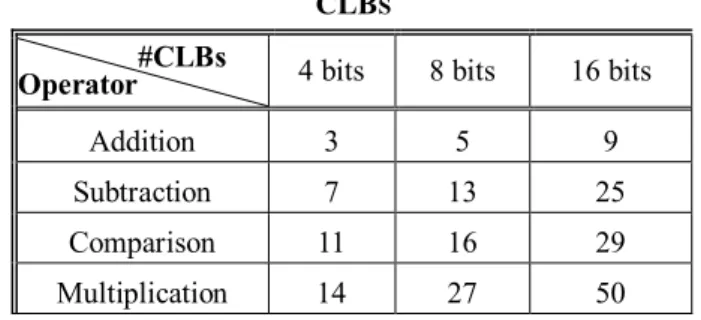
By the above equations, the Viterbi algorithm requires a large number of multiplications to extract the state sequence. From the standpoint of hard-ware design, minimizing the number of multipliers optimizes the architecture. Because a multiplier occupies a large logical block (a large number of CLB), the area cost of the hardware is increased by using many multipliers. For example, it can be seen in Table I that the CLB number of a multiplier is greater than that of an adder. Therefore, we perform the Viterbi algorithm in the logarithm domain so that multiplication operations can be replaced by addition operations.
The Log-Viterbi algorithm is described as fol-lows: ) ( ) ( 1 1 j j bj o for t = 1, 1 j N. (4) ) ( ] ) ( [ max ) ( 1 0 i N t ij j t t j i a b o for 2 t T, 1 j N. (5)
Denote D as the feature order and represent ot =
[ot1, ot2,…, otD] as the observation vector received
in time-step t. In continuous mixture density HMM, an observation probability bj(ot) for the observation
vector ot in the state j can be represented as:
D k jk jk tk D k jk D t j o o b 1 2 2 2 1 1 ) ( exp ) 2 ( 1 ) ( (6)where jk and jk are the mean vectors and diagonal
covariance matrices, respectively, for the state in-dex j and the dimension inin-dex k. Equation 6 is transformed into the logarithm domain as follows:
log bj(ot) =
D k jk D 1 ) 2 ( 1 log +
D k jk jk tk o 1 2 2 2 ) ( = Cj +
2 1 ) ( ~
D k jk tk jk o (7) where Cj =
D k jk D 1 ) 2 ( 1 log and 2 2 1 ~ jk jk B. Operation Weight in HMM DFGIn this subsection, the operations involved in HMM probability evaluation will be organized by a data flow graph (DFG). The DFG, G = (V, E, W), consists of |V| nodes and |E| edges, where each node represents an operation and each edge eE represents a dependence between nodes. For each node vV, there exists a weight wW. The DFG formulation will be discussed in greater detail in Section III.The HMM algorithm operation set which includes addition, subtraction, comparison, and multiplication. In a DRC system, these opera-tions are implemented by configurable logic blocks (CLBs) [6]. An operation may need several CLBs. Take the observation probability generation for example. It has a set of operations that can be rep-resented by DFG, where a node corresponds to an operation and an edge corresponds to the opera-tion’s relation. DRC performance of 4-bit multipli-cation, subtraction and addition are implemented respectively by 14 CLBs, 7 CLBs and 3 CLBs [4]. Since the weight w is the number of CLBs in a node, the respective weights are w(mult) = 14,
w(sub) = 7 and w(add) = 3. Detailed discussion is
III. PROBLEM FORMULATION
A. Motivation
Minimizing the hardware execution time to per-form the HMM algorithm in a PRC system is a primary goal in this paper. To quantify the execu-tion time, every mapped DRPPU process in the HMM DAG is assumed to require a constant and equal unit cycle time, which includes both the re-configuration and execution times for that DRPPU process. Each DRPPU is implemented in a single FPGA. All the FPGA’s have equal size and equal performance capabilities. If we treat the CLB utili-zation of each DRPPU as equal, then the total number of CLBs in a DRPPU is equal. The task of a DRPPU is designed to be completed in a single cycle, after which a new configuration is invoked. For DRPPU run in parallel (Section IV below), we define the total execution time as Texe = k
(DRPPU reconfiguration time) + k (DRPPU
exe-cution time), where k is the number of
configura-tions, i.e. non-parallel DRPPU used in the graph. Recall that a configuration executes the DRPPU process in one cycle, which we will use in the fol-lowing as a standard cycle. Hence, an application’s total execution time is equal to k cycles.
The PRC hardware architecture will be consid-ered in this study. Partitioning methods for the ar-chitecture will be considered. For PRC arar-chitecture, consideration of parallel processing in temporal partitioning improves execution time. In this con-text, the challenge is to exploit the parallelism in-herent in HMM. Importantly, operation duplication in a given application is usually allowed in a paral-lel partitioning solution. Hence, a partitioning tech-nique is developed with this parallel processing consideration in mind. Where a layer is defined as a counter for a parallel array of DRPPU at one cycle time, the depth of a solution is defined as the total number layers in the solution. Optimizing a PRC solution finding a minimum depth duplica-tion-permitted solution. Thus, a HMM DAG is par-titioned into sub-graphs (each representing a DRPPU under one configuration) with a minimum depth solution. Each sub-graph consists of a set of clustered sub-graphs. Each sub-graph is selected by the greedy method, one at a time. This method will be shown to find the minimum depth partitioning of
the HMM algorithm.
B. Terminologies and Problem Formulation
The different states of an HHM can be repre-sented by a directed acyclic graph (DAG), G = (V,
E, W), where V is a set of n nodes and E is a set of
edges. A primary input (PI) node, which has no in-coming edge, represents an input signal. A
pri-mary output (PO) node, which has no out-going
edge, represents an output signal. Except for PI and PO nodes, each node in V represents the imple-mentation of a functional operation such as addi-tion or subtracaddi-tion. Figure 2(a) gives an example of a DAG representing a HMM application, in which nodes a, b, c, d, e, f, g and h are PI nodes and nodes
o, w and t are PO nodes. A directed edge eij = <vi,
vj>, eijE exists if the function input represented by
vj depends on the function output represented by vi.
For each node vi in a node set V, viV, there exists
a weight wiW that represents DRPPU area of
functional operation implementation, vi. Notice that
the weight for every PI and PO node is zero.
Although DAGs have been used in many prior studies of RC systems, most of them dealt with se-rial processing. This presented study uses DAGs to deal with parallel processing issues. To do so, this study introduces the concept of a block, which we use to designate subsets (subgraphs) of the DAG that can be performed independently and in parallel with each other. A block B is a set of nodes VB
which comprise that block. Nodes within VB can be
any of the nodes within a DAG except the PI and PO nodes. In the following diagrams, nodes are designated by single circles and blocks are desig-nated by circles enclosed in dotted lines, as seen in Fig. 2(a). We define the area of any block B as the sum of the weights of the nodes of that block. Since the weight of a node equals the number of CLB in a node, then the area of a block also equals the num-ber of CLB in the block, also called the DRPPU logic capacity, ADRPPU, of any B. Any B is
consid-ered feasible if the area of B ( AB =
B
v b
w ) is less
than or equal to the DRPPU logic capacity, ADRPPU,
i.e. AB ADRPPU. In Figure 2(a), for example, the
block F including nodes z, l, n, and s is feasible if
ADRPPU = 23.
must be scheduled in a block no later than all its output nodes. This is a temporal constraint. Con-straints which determine the temporal ordering of the nodes in the DAG are called precedence
con-straints [4]. Even when a graph is acyclic, blocks
may exist in a cyclic-relation and cannot satisfy precedence constraints after partitioning. A set of feasible blocks in which precedence constraints are satisfied is called a feasible partitioning solution.
In PRC parallel processing reconfigurable archi-tecture, a given DAG is partitioned into feasible blocks such that each block can be implemented in a single DRPPU. The processing of blocks at the same time is allowed up to a maximum for the hardware; in our current example, each DRPPU is implemented by a single FPGA, so the maximum number of blocks that can be processing at the same time equals the number of FPGA. The FPGA (and therefore the blocks) that can be executed in one cycle we designate as a “layer.”
Therefore, the PRC partitioning problem for depth optimization can be formulated as a graph-based problem as:
Given an HMM DAG and the allowing parallel concurrent number of DRPPUs and with re-spect for the maximum number of parallel concurrent number of DRPPUs, find a feasible partitioning solution with a minimum depth number.
(a)
(b)
Fig. 2. DAG of a program or application.
IV. PROPOSED PARALLEL PARTITIONING FOR M
AP-PING HMMDAG ONTO PRC
This section discusses using a single root floor cone to partition a graph so as to have minimum depth. After this, the node duplication effect (an important factor in depth determination) is dis-cussed. The greedy method will be used to find the partitioning solution for a DAG, G = (V, E). Par-ticularly, we consider iteration using the greedy method to select feasible floor cones leads to find the minimum-depth partitioning solution.
A. Floor Cone Properties and Node Duplication
A feasible block B= (V, E) is called a feasible
cone if there exists a node v V such that for every
node uB there is a directed path from u to v in B. The node v is called the root of the floor cone. If all the cone’s fan-in nodes are PI nodes, the feasible cone is called a floor cone. Let Cu = (Vu, Eu) and Cv
=(Vv, Ev) be two cones. Cu and Cv are said to
over-lap if Vu Vv .
Let Cv be a feasible floor cone tipped at v. If a
feasible floor cone tipped at every successor of v is not feasible, Cv is called a maximum floor cone
(MFC). For example, in Figure 4(a) if ADRPPU = 23,
the floor cone including the nodes {x, k, i, r, q} is a MFC. On the other hand, the floor cone including the nodes {k, r} is a floor cone but not a MFC be-cause x is a successor of k and the floor cone tipped at x is a feasible floor cone. Clearly, the MFCv of
node v is a maximal floor cone. Moreover, an MFC has the following important properties.
Lemma 1: If w MFCv, then floor cone Cw
MFCv.
Proof: For any node u Cw, if a path does not exist
from u to root w, it contradicts the assumption that Blocks (layer) C (1) E, F (2) wz x 11 3 i 3 r 3 3 feasible block c d o 0 0 0 0 C E G 0 11 3 l 3 m 3 e w 0 0 0 z 1 1 n 3 s 3 3 t 0 0 F 0 g h f b a p q j y k
u Cw. Therefore, for every node u Cv, there is a
directed path from u to v in Cv. This implies that for
every node w MFCv there is a directed path from
w to v in MFCv. Therefore, Cw MFCv.
Lemma 2: If Vo = MFCv MFCw and u Vo , then
floor cone Cu Vo.
Proof: If MFCv and MFCw exist and overlap Vo ,
then u Vo. Therefore, two paths must exist from u
to v and w. This implies that u MFCv , u
MFCw , and because of Lemma 1, then Cu MFCv
and Cu MFCw.
Node duplication performance uses a DRPPU to cover a MFC that contains an overlapped region. Node duplication is generally very important to depth optimization because duplication usually in-creases DAG parallelism. Without node duplication, many multiple fan-out nodes may have to be ex-plicitly implemented with DRPPUs, possibly caus-ing large depth in the partitioncaus-ing solution. Hence, these feasible cones are allowed to overlap, which means that nodes in the overlapped region must be duplicated when mapping DRPPUs. In fact, in or-der to achieve depth optimization, our algorithm is capable of duplicating nodes automatically when necessary.
Traditionally in DRPPU temporal partitioning, a graph is partitioned into several sub-graphs. The previously proposed algorithms [3] and [4] do not consider whether sub-graphs have parallelism or not. We consider that if the sub-graphs have inher-ent parallelism, after which we organize the prop-erly-partitioned sub-graphs so that they can be executed during the same cycle, thereby improving performance.
B. MFC-Processing for DRPPU Capacity
In the preceding discussion we presented tech-niques for minimizing the depth in parallel parti-tioning. Assuming that the maximum parallelism of a given array is k (in this case, the number of FPGA in our simulated prototype’s parallel array; in a more general case, this is the number of DRPPU in the array), then after finding all feasible floor cones to the mapped k DRPPUs, we still cannot be sure each MFC represents the maximal capacity of the DRPPU. Thus we define the maximal mapping
graph MMG to be a set of MFCs such that MFC
MMG. The objective of MFC-processing in our parallel partitioning algorithm is to find k MMG (k-MMGs) by selecting all MFCs that can be col-located under the DRPPU k capacity constraint (i.e. ≤ k) and to confirm that the MFCs can collocate in a single layer.
On the other hand, it should be noted that MFC-processing affects the depth, i.e. the number of layers in the design. Since increasing the number of layers increases the execution time of the design, it is desired to minimize the depth. This is accom-plished by use of a bin-packing technique which treats the problem as a matter of minimizing the number of MMGs per MFC set. Since there are m MFCs in a MFCs set, the size of each MFC is ci
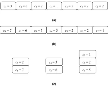
which is a positive integer. We further give positive integers B and C as the number of bins and the bin capacity, respectively. The bin packing problem determines the minimum number of bins which can accommodate all m items. In general, the goal of bin packing is to find the minimum number of bins into which a set of boxes can be packed. In this case the bin packing problem is NP-complete, with the bins corresponding to the number of the DRPPUs and the boxes corresponding to the set of MFCs. The capacity of each bin is C, and the size of each box is the area size of the MFC. Herein, the bin packing algorithm used is First Fit Decreasing (FFD).
Figure 3(a) shows an example of the set of the MFCs. There are seven MFCs in G, with each floor cone having size weight c1 = 3, c2 = 6, c3 = 2, c4 = 1,
c5 = 5, c6 = 7 and c7 = 2 respectively. If the bin
ca-pacity of C is 9 then each floor cone corresponds to box capacity ci, where 1 i 7. First, we sort
ob-jects so that ci ci+1, 1 i 7 as shown in Figure
3(b) and then pack object i in bin j where j is the least index such that bin j can contain object i. In Figure 3(c) the final contents of the packed bins are 9, 9 and 8, such that B = 3.
Hence, the number of MFCs is decreased by ap-plying bin packing as an MFC-processing step. When the number of bins is more than the k-MMG, we choose the k number of the largest capacity in bin B. There are other methods that can further de-crease area cost after the MFCs have been pro-duced.
(a)
(b)
(c)
Figure 3. (a) A set of MFCs; (b) Sorting these MFCs; (c) Reducing the number of MFCs according to the bin packing FDD.
Alternative partitioning methods and their dif-ferent results have been presented above. It has been shown that the objective is a minimum num-ber of layers when a graph G is partitioned by ap-plying ≤k number of MMG’s.
Theorem 1: If a DAG is partitioned by MFC with
consideration of the ≤k-MMGs, then the result of partitioning is an optimal depth solution.
Proof: Given a graph G and in a PRC system with k
DRPPU, G is partitioned into subgraphs to find the depth. Based on Lemmas 1 and 2, we can obtain every MFC with an optimal solution. Hence in graph G, k-MMG was found by the all MFCs. Ac-cording to the MMG definition, each MMG mapped to a DRPPU has maximal area. Let Sg be a
set of MMGs. Now we use divide and conquer to obtain the solution. For graph G, after we find
k-MMG’s Sg, the new graph G is produced by the
procedure, G = G – Sg. Recursively, the step of
finding k-MMG’s Sg until all node have been
proc-essed in graph G. It means that the minimum-depth solution of G is the union of {Sg} and the
mini-mum-depth solution of G – Sg. Hence, account of
the depth is an optimal solution since each step of finding k-MMG’s is an optimal solution.
C. The Minimizing Depth Algorithm
A PRC parallel partitioning algorithm is pre-sented in this subsection. Determining every MFC in a graph is first introduced. Then the minimum depth obtained recursively by obtaining k-MMGs is
explained. Assume that the area constraint is 23, i.e.
ADRPPU = 23. For example, 3-MFCs including Cx,
Cy and Cz in Figure 2 can be selected for the
opti-mal solution, where 3-MFCs is equal to 3-MMGs. The minimizing depth algorithm is given in Fig. 4. The algorithm needs to find all feasible floor cones to determine k-MMGs. The major work of parallel partitioning is to find every MFC in G. In every floor cone graph, there are three steps, namely calculating the area, sorting the area, and the labeling nodes. Application of the traversal technique applies a depth first search (DFS) for calculating the floor cone area. A floor cone is con-structed with the node as a root if the floor cone is feasible. In the second step the sorting technique uses MergeSort. Moreover, we label the chosen root v and its predecessors, Pre (v) to get the Sc set,
where Sc is a set of MFCs. Let TP (v) =
) ( Prev u u C . Based on the Sc set, our parallel algorithm can find
k-MMGs such that the k-MMGs, Sg is obtained by
using FFD method in the MFC-processing. When a new DAG G = G – Sg is obtained, we return to the
generate-MMG’s step in the partitioning procedure to find the new depth of the feasible cone. New MMGs are generated to increase the number of depths so that the partitioning depth in graph G in-creases until all nodes is covered to the MFC. Algorithm Determining Depth:
FindMinimumDepth(G)
Comment: G(V, E) is a directed acyclic graph depth = 0;
L = ; SortList = ; Sc = ; Sg = ;
for every node u in G
L: = List L of all of nodes in topological order; end of the for loop
while (L ) do
for every node v in G do; CalculateArea(Cv) by DFS; if Area(Cv) ADRPPU then do SortList Cv
end of the for loop while (SortList ) do
Sort area of SortList by MergeSort for every floor cones Cv in SortList do if Cv is the MFC then
Sc = Sc Cv;
L = L – {v Pre(v)};
SortList = SortList – {Cv TP(v)}; end of the if loop
c7 = 1 c3 = 5 c4 = 3 c2 = 6 c1 = 7 c5 = 2 c6 = 2 c4 = 1 c5 = 5 c3 = 2 c2 = 6 c6 = 7 c1 = 3 c7 = 2 c4 = 3 c5 = 2 c3 = 5 c2 = 6 c6 = 2 c1 = 7 c7 = 1
end of the while loop for every MFC in Sc Finding Sg by FFD; end of the for loop G = G – Sg; Sg = ; Sc = ;
depth = depth + 1; end of the while loop
Figure 4. The minimum-depth algorithm for parallel partitioning
D. The Complexity of the Algorithm
The whole partitioning procedure has a low time complexity. Before finding the MFC, all the nodes are processed by topological sorting. Hence during portioning, the nodes are visited in topological or-der. The time complexity of visiting the nodes is O(VlogV) where V is the number of nodes in the given graph. The task of finding each MFC in-cludes calculating the area, sorting the area and la-beling nodes. Each floor cone area is calculated by the depth first search (DFS) methodology. Hence, the time complexity of calculating the area is O(VlogV). In sorting the area, the number of floor cones is no more than the number of nodes V. The time complexity is O(V). When labeling nodes, a node is visited once. The complexity of labeling nodes is O(V). In the MFC-processing, to apply FFD the number of MFC is no more than the number of nodes V. The time complexity is O(VlogV). The minimum-depth partitioning solution selects k-MMG’s in each greedy method iteration. Therefore, depth determining takes O(V2logV) time. In conclusion, the total time complexity is bounded by O(V2logV).
V. EXPERIMENTAL RESULTS
The proposed PRC partitioning algorithm was implemented in C language on a Blade 1000 work-station. For performance evaluation the algorithm was assigned to partition a published DAG for an HMM algorithm. We derive 4 DAGs for this algo-rithm for four different levels of HMM complexity, i.e. for four different state numbers. Since higher state numbers imply much larger DAGs, this chal-lenges the ability of our algorithm to minimize depth. Also, since algorithm depth is directly re-lated to application execution speed, this is a good
demonstration of the speed improvement that can be obtained by PRC.
Our proposed algorithm can compute a theoreti-cally unlimited number of parallel FPGA modules (DRPPU) but, for reasons of simple comparison, we perform simulations for parallel arrays from one to 5 DRPPU and for DRPPU areas (ADRPPU) from
1536, 2304, 2688, 4992, 6144, 6656 to 9280 CLB. Thus we are demonstrating the ability of our algo-rithm to help design massively parallel architecture. In fact, FPGA is intrinsically capable of such func-tion but applicafunc-tion up to the present time has been largely linear, due to lack of design tools and the habitual persistence of traditional thinking. It will be seen that speed optimization is obtained by use of larger DRPPU numbers. Functional operations such as addition, subtraction, multiplication are implemented by CLBs of a DRPPU. Table I shows the number of CLBs in each of these basic opera-tions, while columns 2 to 4 show the different bit widths. The following data present the results of using our algorithm to mapping HMM DAGs of varying state numbers onto PRC architecture. The HMM state numbers mapped are 4, 8, 12 and 24. Here we use PRU abbreviation to present the DRPPU in the below Table and Figure.
TABLE I.AREA OF THE OPERATIONS EXPRESSED IN XC4000 CLBS
#CLBs
Operator 4 bits 8 bits 16 bits
Addition 3 5 9
Subtraction 7 13 25
Comparison 11 16 29
Multiplication 14 27 50
The results of partitioning the HMM (2 DAGs, 8 and 24 states) is presented in Fig. 5, with results given as minimum depth for each state conditions for a given number of parallel processing units (# of DRPPU), where each DRPPU group is subdi-vided into ADRPPU (DRPPU area, i.e. number of
CLB per DRPPU). Note that when the number of DRPPU equals one, this indicates a single FPGA which is equivalent to non-parallel processing. This value is given for comparison and to demonstrate
the capability of the presented algorithm. In Fig. 5, it is obvious that the depth decreases (i.e. the speed increases) as the number of DRPPU increases and also as the number of CLB per DRPPU increases.
Performance Evaluation 8-states 0 2 4 6 8 10 12 14 1 2 3 4 5 #PRU #D ep th RPU-1536 RPU-2304 RPU-2688 RPU-4992 RPU-6144 RPU-6656 RPU-9280 (a) Performance Evaluation 24-states 0 2 4 6 8 10 12 14 16 18 20 1 2 3 #PRU 4 5 #D ep th RPU-1536 RPU-2304 RPU-2688 RPU-4992 RPU-6144 RPU-6656 RPU-9280 (b)
Fig. 5. Evaluation results of architecture performance based on depth number: (a) 8-state HMM; (b) 24-state HMM.
Finally, we compare the speed performance of the same HMM implementation in different archi-tectures. This is presented in Tables II and III. Columns 2 to 4 respectively show the Texe for the
same HMM as implemented by general purpose processing (GPP), parallel processing elements without the local memory of DRPPU (Fig. 1(a)) and the PRC method with fully equipped DRPPU. Performance comparison is based on time-step execution time Texe analysis of the results of a 4-, 8-,
12- and 24-state speech recognition Viterbi HMM algorithm decoder in C running on a Core 2 1.86GHz CPU 2GB RAM machine with the each time-step of the execution time assigned to 10 ms.
Table II shows the results for PE and DRPPU con-sisting of 1536 CLB each. For the 4-, 8-, 12- and 24-state HMM implementations, the proposed PRC design demonstrated average 12.26 and 3.53 exe-cution time improvement relative to the GPP and the PE designs. Table III compares these systems when the computing block capacity is 2688 CLBs. Here PRC showed relative execution time im-provements of approximately 17.12 and 3.36 with respect to the GPP and PE designs. The major im-provement observed for the proposed PRC archi-tecture (Fig. 1(a)) adopted in our DRPPU is attrib-utable to the faster reconfiguration time resulting from the virtue improved bus cycle time.
TABLE II.COMPARISON OF DIFFERENT DESIGNS FOR EXE-CUTION TIME (NS) Improvement Time States GPP Parallel (1536clbs) PRC (1536clbs) GPP Parallel 4-states 10000 2910 660 14.15 3.41 8-states 10000 2970 660 14.15 3.50 12-states 10000 4000 880 10.36 3.55 24-states 10000 4120 880 10.36 3.68 Average 12.26 3.53
TABLE III.COMPARISON OF DIFFERENT DESIGNS FOR EXE-CUTION TIME (NS) Improvement Time States GPP Parallel (2688clbs) PRC (2688clbs) GPP Parallel 4-states 10000 1950 460 20.74 3.24 8-states 10000 1990 460 20.74 3.33 12-states 10000 3015 690 13.49 3.37 24-states 10000 3120 690 13.49 3.52 Average 17.12 3.36 VI. CONCLUSIONS
The addition of parallel processing techniques to reconfigurable computing has the potential to im-prove DSP applications. Therefore, multiple proc-essing units arranged according to traditional par-allel processing techniques are being applied for high computation and data intensive applications such as HMM. This paper has presented a mini-mum-depth partitioning algorithm for parallel re-configurable computing. It is shown that applica-tion speed can be improved by increasing parallel-ism of the parallel DRC units. The resulting
high-parallelism design has somewhat higher total chip area because of redundancy between parallel units. The proposed algorithm can accept arbitrary chip area constraints or maximum parallelism con-straint and then optimize for speed.
REFERENCE
[1] J. Noguera and R. M. Badia, “HW/SW Codesign Techniques for Dynamically Recon-figurable Architectures,” IEEE Transactions on
VLSI, vol. 10, pp. 399-415, Aug. 2002.
[2] T. Fujii et al, “A dynamically reconfigurable logic engine with a multiconfiguration/ multi-mode unified-cell architecture,” in Proc.
IEEE Int. Solid-State Circuits Conf., 1999, pp.
364-365.
[3] G. M. Wu, J. M. Lin, and Y. W. Chang, “Generic ILP-based approaches for time-multiplexed FPGA partitioning,” IEEE Trans. Com-puter-Aided Design, vol. 20, no. 10, pp.
1266-1274, Oct. 2001.
[4] Y. C. Jiang and J. F. Wang, “Temporal Parti-tioning Data Flow Graphs for Dynamically Re-configurable Computing,” IEEE Transactions
on VLSI, vol. 15, no. 12, pp. 1351-1361, Dec.
2007.
[5] W. Stallings, “Computer organization and ar-chitecture: designing for performance,” Pearson Education, 2003.
[6] [Online]. Available: http://www.xilinx.com/ [7] L. F. Chen, Y. K. Lai, “VLSI architecture of the
reconfigurable computing engine for digital signal processing applications,” IEEE Circuits
and Systems Conference., ISCAS '04. pp.
937-40, May 2004.
[8] Vissers, K. A, “Parallel processing architectures for reconfigurable systems,” Design, Automa-tion and Test in Europe Conference and Exhibi-tion, 2003 pp. 396 - 397
[9] H. Schmit et al, “PipeRench: A virtualized pro-grammable datapath in 0.18 micron technol-ogy,” IEEE Custom Integrated Circuits
Con-ference., pp. 63-66, May 2002.
[10] H. Singh, G. Lu, M. Lee, F. J. Kurdahi, N. Bagherzadeh, E. Filho, R. Maestre, “Morpho-Sys: Case Study of a Reconfigurable Comput-ing System TargetComput-ing Multimedia Applica-tions,” Proceedings Design Automation
Con-ference (DAC’00), pp. 573-578, Los Angeles,
California, May 2000.
[11] R. Maestre, F. J. Kurdahi, M. Fernández, R. Hermida, N. Bagherzadeh, H. Singh, “Kernel Scheduling Techniques for Efficient Solution Space Exploration in Reconfigurable Comput-ing,” Special Issue on Modern Methods and Tools in Digital System Design, in the Journal
on System Architecture, 47, pp. 277-292, 2001.
[12] S. A. Fahmy, Peter Y. K. Cheung and W. Luk, “Hardware acceleration of Hidden Markov Model decoding for person detecction,” Design, Automation and Test in Europe Conference and Exhibition, 2005, pp. 8-13.
[13] Y. Zhu and M. Benaissa, “A novel acs scheme for area-efficient viterbi decoders,” In Proc. IEEE International Symposium on Circuits and Systems. ISCAS ’03., vol. 2, pp. 264–267, May 2003.