The Electrophoretic Mobility and Electric Conductivity of a Concentrated
Suspension of Colloidal Spheres with Arbitrary Double-Layer Thickness
Jau M. Ding and Huan J. Keh1
Department of Chemical Engineering, National Taiwan University, Taipei 106-17, Taiwan, Republic of China
Received August 17, 2000; accepted December 4, 2000
The electrophoresis in a monodisperse suspension of dielectric spheres with an arbitrary thickness of the electric double layers is analytically studied. The effects of particle interactions are taken into account by employing a unit cell model, and the overlap of the double layers of adjacent particles is allowed. The electroki-netic equations, which govern the ionic concentration distributions, the electric potential profile, and the fluid flow field in the elec-trolyte solution surrounding the charged sphere in a unit cell, are linearized assuming that the system is only slightly distorted from equilibrium. Using a perturbation method, these linearized equa-tions are solved with the surface charge density (or zeta potential) of the particle as the small perturbation parameter. Analytical ex-pressions for the electrophoretic mobility of the colloidal sphere in closed form correct to O(ζ) are obtained. Based on the solution of the electrokinetic equations in a cell, a closed-form formula for the electric conductivity of the suspension up to O(ζ2) is derived from the average electric current density. Comparisons of the results of the cell model with different conditions at the outer boundary of the cell are made for both the electrophoretic mobility and the electric conductivity. °C2001 Academic Press
Key Words: electrophoretic mobility; electric conductivity; con-centrated suspension; unit cell model; arbitrary double-layer thick-ness.
1. INTRODUCTION
A charged colloidal particle suspended in an electrolyte so-lution is surrounded by a diffuse cloud of ions carrying a total charge equal and opposite in sign to that of the particle. This dis-tribution of fixed charge and diffuse ions is known as an electric double layer. When an electric field is imposed on a suspension of charged particles, a force is exerted on both parts of each dou-ble layer. The particles are attracted toward the electrode of their opposite sign, while the ions in the diffuse layers migrate in the other direction. This particles’ motion is called electrophoresis and has been applied to the particle characterization and sepa-ration in a variety of colloidal and biological systems. On the other hand, the fluid is dragged to flow by the motion of the par-ticles and the ions, and there is an electric current through the
1To whom correspondence should be addressed. E-mail: [email protected]. edu.tw. Fax: +886-2-2362-3040.
suspension to produce. To find out the transport properties such as the average electrophoretic mobility or the effective electric conductivity of the suspension, it is necessary to first determine the distributions of the electric potential, ionic concentrations, and fluid velocity in the electrolyte solution.
The first analysis on electrophoresis of a particle which took into account the finite thickness of the electric double layer was conducted by Henry (1). Assuming that the double layer is not distorted from the equilibrium state, he derived an analytical ex-pression for the electrophoretic mobility of a dielectric sphere (and of an infinitely long cylinder) of radius a with small zeta potentialζ for the entire range of κa, where κ−1 is the Debye screening length. For the two extreme cases κa → ∞ and κa → 0, this result reduces to the well-known Smoluchowski equation and Huckel expression, respectively. Later, Booth (2) extended Henry’s analysis to include the effect of ionic con-vection in the diffuse layer and determined the electrophoretic mobility of a charged sphere as a power series in ζ. Taking the double-layer distortion from equilibrium as a perturbation, O’Brien and White (3) improved an earlier attempt made by Wiersema et al. (4) to obtain a numerical calculation for the electrophoretic mobility of a dielectric sphere in electrolyte so-lutions which was applicable to arbitrary values ofζ and κa. The numerical results show that the polarization effect (or relaxation effect) of the double layer impedes the particle’s movement be-cause an opposite electric field is induced in the distorted ion cloud, which acts against the motion of the particle. This polar-ization effect vanishes for the situation of very lowζ and for the two limiting casesκa → ∞ and κa → 0.
The basic electrokinetic equations describing the elec-trophoretic phenomena in a suspension of colloidal particles also govern the effective electric conductivity of the suspension. Dukhin and Derjaguin (5) derived a simple formula for the elec-tric conductivity of a dilute suspension of charged particles by considering an infinite plane slab of suspension immersed in an infinite homogeneous electrolyte subjected to an electric field perpendicular to the plane slab. Extending this analysis, Saville (6) and O’Brien (7) assumed that the particles and their electric double layers occupy only a small fraction of the total volume of the suspension to obtain approximate formulas for the ef-fective conductivity using a perturbation method for particles with low ζ immersed in a symmetrically charged electrolyte 180
0021-9797/01 $35.00
Copyright°C2001 by Academic Press All rights of reproduction in any form reserved.
correct to O(ζ2). Their results show some discrepancies with the experimental data reported by Watillon and Stone-Masui (8), who measured the surface conductances of a number of monodisperse polystyrene latices over a range of particle vol-ume fractions. Later, approximate analytical expressions for the electrophoretic mobility and the electric conductivity of dilute suspensions of colloidal spheres in symmetric electrolytes cor-rect to order (κa)−1were obtained by Ohshima et al. (9). When the zeta potential of the particles is small, their reduced result is in agreement with those of Henry (1) and O’Brien (7). Re-cently, analytical expressions for the electrophoretic mobility and the electric conductivity of dilute suspensions of charged porous spheres (10) and charged composite spheres (11) with an arbitrary value ofκa were derived under the assumption that the densities of the particles’ fixed charges are low.
In practical applications of the electrophoretic mobility and the effective electric conductivity, relatively concentrated suspensions of particles are usually encountered, and effects of particle interactions will be important. To avoid the difficulty of the complex geometry appearing in assemblages of particles, unit cell models were often employed to predict the effects of particle interactions on the mean sedimentation rate in a bounded suspension of identical uncharged spheres (12). These models involve the concept that an assemblage can be divided into a number of identical cells, one sphere occupying each cell at its center. The boundary value problem for multiple spheres is thus reduced to the consideration of the behavior of a single sphere and its bounding envelope. The most acceptable of these models with various boundary conditions at the outer (virtual) surface of a spherical cell are the so-called “free-surface” model of Happel (13) and “zero-vorticity” model of Kuwabara (14), the predictions of which have been tested against the experimental data. Using the Kuwabara cell model, Levine and Neale (15) derived a complicated analytical expression for the elec-trophoretic mobility in a suspension of identical charged spheres with smallζ and arbitrary κa as a function of the fractional vol-ume concentration of the particles. In the limiting case of a dilute suspension, their result reduces to that obtained by Henry (1). Later, the Kuwabara cell model was also used by Davis and co-workers (16–18), Ohshima (19, 20), and Lee et al. (21) to predict the electrophoretic mobility of charged spheres in concentrated suspensions and/or the electric conductivity of the suspensions. All the previous analyses for the electric conductivity of sus-pensions of charged particles using the cell model (16, 18, 20) were based on the assumption that the overlap of the adjacent double layers is negligible on the virtual surface of the unit cell. With this assumption, the effect of the relaxation of the diffuse ions in the double layer within a cell due to the electrophoretic motion of the particle, at best, can only be described by sim-ple approximations. Therefore, the application of their results is restricted to the case of charged spheres with relatively thin double layers (e.g.,κa ≥ 10). On the other hand, the Kuwabara cell model was chosen in the previous studies (15–21) because it could predict that the electrophoretic mobility in a bounded
suspension of identical spheres withκa → ∞ is independent of the volume fraction of particles, while the corresponding pre-diction of the Happel cell model gives a weak dependency of the mobility on the particle concentration, and because its zero-vorticity boundary condition is consistent with the irrotational-flow environment generated by an electrophoretic particle with κa → ∞. In the analysis based on the concepts of interactions between pairs of electrophoretic spheres and statistical mechan-ics (22–24) and in a careful experimental study (25), however, it was found that the electrophoretic mobility in a bounded suspen-sion of identical spheres at largeκa decreases gradually rather than remaining unchanged with increasing volume fraction of particles. Also, the fluid flow dragged by an electrophoretic par-ticle surrounded by a double layer with a finite thickness is no longer irrotational. In fact, the Happel model has a significant advantage over the Kuwabara model in that the former does not require an exchange of mechanical energy between the cell and the environment (12).
In this work, the unit cell model is used to derive the elec-trophoretic mobility in a relatively concentrated suspension of identical charged spheres and the electric conductivity of the sus-pension. The overlap of adjacent double layers is allowed and, for the evaluation of the electric conductivity, the relaxation ef-fect in the diffuse layer surrounding each particle is taken into account appropriately. The surface charge density (or zeta po-tential) of the dielectric particle is assumed to be uniform, but no assumption is made about the thickness of the double layer relative to the dimension of the particle. Both the Happel model and the Kuwabara model are considered. In the next section, we present the fundamental electrokinetic equations and boundary conditions which govern the electrolyte ion distributions, the electrostatic potential profile, and the fluid flow field in a unit cell. These basic equations are linearized assuming that the ion concentrations, the electric potential, and the fluid pressure show only a slight deviation from equilibrium due to the application of the electric field. In Section 3, the electrophoresis of the charged sphere in a cell containing an arbitrary electrolyte solution is considered. Using the Debye–H¨uckel approximation, we first get the solution of the equilibrium electric potential distribution. The linearized electrokinetic equations are then transformed into a set of differential equations by a perturbation method with the surface charge density of the particle as the small perturbation parameter. The perturbed electrochemical potential, fluid veloc-ity, and pressure profiles are determined by solving this set of differential equations subject to the appropriate boundary condi-tions. A closed-form expression for the electrophoretic mobility of the charged sphere results from satisfying the requirement that the net force acting on the cell vanishes. In Section 4, the average electric current density in a concentrated suspension of identical charged spheres is derived, and an explicit formula for the effective electric conductivity is obtained. Finally, analyt-ical expressions in some limiting cases and typanalyt-ical numeranalyt-ical results of the electrophoretic mobility and electric conductivity for a suspension of charged spheres are presented in Section 5.
Comparisons of the previous analyses neglecting the overlap of the adjacent double layers and some experimental results with our calculations are made.
2. BASIC ELECTROKINETIC EQUATIONS
We consider a statistically homogeneous distribution of iden-tical charged spherical particles in a bounded liquid solution containing M ionic species. When the suspension is subjected to a uniform applied electric field E∞ez, the colloidal particles
migrate with a velocity equal to U ezat the steady state due to
electrophoresis, where ezis a unit vector (in the positive z
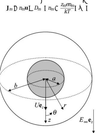
direc-tion). Gravitational effects are ignored. As shown in Fig. 1, we employ a unit cell model in which each particle of radius a is surrounded by a concentric spherical shell of suspending solu-tion having an outer radius of b such that the particle/cell volume ratio is equal to the particle volume fractionϕ throughout the entire suspension; viz.,ϕ = (a/b)3. The cell as a whole is elec-trically neutral. The origin of the spherical coordinate system (r, θ, φ) is taken at the center of the particle and the axis θ = 0 points toward the positive z direction. Obviously, the problem for each cell is axially symmetric about the z-axis.
Conservation of all ionic species, which do not react with one another, requires that
∇ · Jm= 0, m = 1, 2, . . . , M, [1]
where Jm(r, θ) is the number flux distribution of species m. If
the solution is dilute, the flux is given by
Jm= nmu− Dm µ ∇nm+ zmenm kT ∇ψ ¶ , [2]
FIG. 1. Geometric sketch of a spherical particle undergoing electrophoresis at the center of a spherical cell.
where nm(r, θ), Dm, and zmare the concentration (number
den-sity) distribution, diffusion coefficient, and valence, respectively, of species m; u(r, θ) is the fluid velocity field relative to the particle; ψ(r, θ) is the electric potential distribution; e is the elementary electric charge; k is Boltzmann’s constant; T is the absolute temperature. The first term on the right-hand side of Eq. [2] represents the convection of the ionic species by the fluid mo-tion and the second term denotes the diffusion and electrically induced migration of the species.
We assume that the Reynolds number of the fluid motion is vanishingly small, so the inertial effect on the fluid momentum balance can be neglected. The fluid flow is governed by the Stokes equations modified with the electrostatic effect,
η∇2u= ∇ p + M X m=1 zmenm∇ψ, [3] ∇ · u = 0, [4]
whereη is the viscosity of the fluid and p(r, θ) is the fluid pres-sure distribution.
The local electric potentialψ and the space charge density are related by Poisson’s equation,
∇2ψ = −4π ε M X m=1 zmenm. [5]
In this equation,ε = 4πε0εr, whereεris the relative permittivity of the electrolyte solution andε0is the permittivity of a vacuum. In Eqs. [2], [3], and [5], Dm, η, and εr, are assumed to be constant in the fluid phase.
The boundary conditions at the surface of the dielectric par-ticle are r= a : u = 0, [6a] er· Jm= 0, [6b] er· ∇ψ = − 4π ε σ, [6c]
where eris the unit normal outward from the particle surface and
σ is the surface charge density of the particle. In Eq. [6a], we have assumed that the “shear plane” coincides with the particle surface. Equations [6b] and [6c] state that no ions can penetrate into the particle and the Gauss condition holds at the surface of the particle. The effect of conductance behind the shear plane is neglected.
At the outer (virtual) surface of the cell, the local electric field is parallel to the uniform applied field E∞ez. Thus, the boundary
conditions there are
r = b : ∂ψ
∂r = −E∞cosθ, [7a] ∂nm
ur = −µEE∞cosθ, [7c] τrθ = η · r ∂ ∂r µ uθ r ¶ +1 r ∂ur ∂θ ¸ = 0
(for the Happel model), [7d] (∇ × u)φ = 1 r ∂ ∂r(r uθ)− 1 r ∂ur ∂θ = 0
(for the Kuwabara model), [7e] whereµEis the electrophoretic mobility of the charged dielectric sphere, and urand uθare the r andθ components, respectively,
of u. Note that the Happel cell model (13) assumes that the radial velocity and the shear stress of the fluid on the outer boundary of the cell are zero, while the Kuwabara cell model (14) assumes that the radial velocity and the vorticity of the fluid are zero there. Because the reference frame is taken to travel with the particle, the radial velocity given by Eq. [7c] is generated by the particle velocity in the opposite direction. The conditions [7c] and [7b] imply that there are no net flows of fluid and ionic species between adjacent cells; they are valid because the suspension of the particles is bounded by impermeable and inert walls. Thus, the effect of the backflow of fluid occurring in a closed container is included in both cell models.
Because the governing equations are coupled nonlinear partial differential equations, it is a formidable task for finding a general solution of them. Therefore, we shall assume that the system is only slightly distorted from the equilibrium state, where the par-ticle and fluid are at rest, and replace these nonlinear equations by approximate linear equations. One can write
p= p(eq)+ δp, [8a]
nm= n(eq)m + δnm, [8b]
ψ = ψ(eq)+ δψ, [8c]
where p(eq)(r, θ), n(eq)
m (r ), and ψ(eq)(r ) are the equilibrium
dis-tributions of pressure, concentration of species m, and electric potential, respectively, andδp(r, θ), δnm(r, θ), and δψ(r, θ) are
the small perturbations to the equilibrium state. The equilib-rium concentration of any species is related to the equilibequilib-rium potential by the Boltzmann distribution,
n(eq)m = n∞m exp à −zmeψ(eq) kT ! . [9]
Here, n∞m is the concentration of the type m ions in the bulk (electrically neutral) solution where the equilibrium potential is set equal to zero. Note thatψ(eq)and n(eq)
m depend on r only due
to spherical symmetry.
Substituting Eq. [8] into Eqs. [1] and [3], canceling their equi-librium components, using Eqs. [5] and [9], and neglecting the
products of the small quantities u,δnm, andδψ, one obtains
∇2δµ m = zme kT µ ∇ψ(eq)· ∇δµ m− kT Dm ∇ψ(eq)· u ¶ , m= 1, 2, · · · , M, [10] η∇2u= ∇δp − ε 4π ¡ ∇2ψ(eq)∇δψ + ∇2δψ∇ψ(eq)¢· [11] Here,δµm is defined as a linear combination of δnm andδψ
based on the concept of the electrochemical potential energy (7),
δµm=
kT n(eq)m
δnm+ zmeδψ· [12]
The boundary conditions forδµmresulting from Eqs. [6] and
[7] and their equilibrium state are
r = a: ∂δµm
∂r = 0, [13]
r = b: ∂δµm
∂r = −zmeE∞cosθ. [14]
The fluid velocity u is a small perturbed quantity, and the bound-ary conditions for u have been given by Eqs. [6a], [7c], and [7d] or [7e].
The boundary condition of the electric potential at the virtual surface r= b may be taken as the distribution giving rise to the applied field E∞ezin the cell when the particle does not exist.
In this case, Eq. [7a] becomes
r= b: ψ = ψ(eq)− E∞r cosθ· [15]
Accordingly, Eq. [14] is replaced by
r = b: δµm= −zmeE∞r cosθ· [16]
Note that in all the previous studies (15–21) on the elec-trophoretic mobility and/or electric conductivity of suspensions of charged particles using the unit cell model Eq. [7a] or [14] has been chosen exclusively as the boundary condition for the potential distribution at the virtual surface of the cell.
3. SOLUTION OF THE ELECTROKINETIC EQUATIONS AND ELECTROPHORETIC MOBILITY
Before solving for the problem of electrophoresis of a charged sphere in a unit cell filled with the solution of M ionic species with constant bulk concentrations n∞m, we need to determine the equilibrium electric potential first. The equilibrium potential ψ(eq)satisfies the Poisson–Boltzmann equation, resulting from the substitution of the Boltzmann distribution [9] into Poisson’s equation [5], the boundary condition [6c], and the requirement
of no electric current passing through the virtual surface r = b at equilibrium. It can be shown that
ψ(eq)= ψ
eq1(r ) ¯σ + O( ¯σ2), [17] where ¯σ = 4πeσ/εκkT , which is the nondimensional surface charge density of the particle, and
ψeq1(r )= kT e µκa A ¶ a r[(κb + 1) exp(κa + κr) + (κb − 1) × exp(κa + 2κb − κr)], [18] with
A= (κb − 1)(κa + 1) exp(2κb) − (κa − 1)(κb + 1) exp(2κa).
[19]
Here, κ is the Debye–H¨uckel parameter equal to (4πe2PmM=1z2mn∞m/εkT )1/2. Expression [17] for ψ(eq) as a power series in the surface charge density of the particle up to O( ¯σ ) is the equilibrium solution for the linearized Poisson–Boltzmann equation that is valid for small values of the electric potential (the Debye–H¨uckel approximation). That is, the surface charge density must be small enough for the potential to remain small. Note that the contribution from the ¯σ2 term toψ(eq)in Eq. [17] disappears for the case of symmetric electrolytes.
To solve for the small quantities u, δp, δψ, and δµm and
the particle mobilityµEfor the case of small parameter ¯σ , these variables are written as perturbation expansions in powers of ¯σ,
u= u1σ + u¯ 2σ¯2+ · · · , [20a] δp = p1σ + p¯ 2σ¯2+ · · · , [20b] δψ = ψ0+ ψ1σ + ψ¯ 2σ¯2+ · · · , [20c] δµm = zmeψ0+ µm1σ + µ¯ m2σ¯2+ · · · , [20d]
µE = µE1σ + µ¯ E2σ¯2+ · · · , [20e] where the functions ui, pi, ψi, µmi andµEi are independent of
¯
σ . The zeroth-order terms of µE, u, and δp disappear because an uncharged particle will not move by applying an electric field. It is easy to show that
ψ0= − E∞ χ µ a3 2r2 + r ¶ cosθ, [21]
where the coefficientχ equals 1 − ϕ when the condition [14] is used, and equals 1+ ϕ/2 when the condition [16] is used.
Substituting the expansions given by Eq. [20] andψ(eq)given by Eq. [17] into the governing equations [4], [10], and [11] and boundary conditions [6a], [7c], [7d] or [7e], [13], and [14] or [16], and equating like powers of ¯σ on both sides of the respective equations, one can derive a group of linear differential equations
and boundary conditions for each set of functions ui, pi, and
µmi, with i equal to 1, 2, . . . . After collecting the first-order
terms in the perturbation procedure, we obtain
∇2u 1= 1 η∇ p1− ε 4πη∇ 2ψ eq1∇ψ0, [22a] ∇ · u1= 0, [22b] ∇2µ m1= − z2 me2E∞ kTχ µ 1−a 3 r3 ¶ dψeq1 dr cosθ, [23] with r= a: u1 = 0, [24a] ∂µm1 ∂r = 0, [24b] r = b: u1r = −µE1E∞cosθ, [25a] τ1rθ = 0 (for the Happel model), [25b] (∇ × u1)φ= 0 (for the Kuwabara model), [25c]
∂µm1
∂r = 0 (if Eq. [14] is used), [25d] µm1= 0 (if Eq. [16] is used). [25e]
The solutions forµm1, p1, and the r andθ components of u1 subject to Eqs. [22]–[25] are
u1r = E∞F1r(r ) cosθ, [26a] u1θ = E∞F1θ(r ) sinθ, [26b] p1 = E∞ · η aFp1(r )− εκ2 4πχ µ r+ a 3 2r2 ¶ ψeq1(r ) ¸ cosθ, [26c] µm1= E∞Fm1(r ) cosθ, [27]
where the functions F1r(r ), F1θ(r ), Fp1(r ), and Fm1(r ) are
de-fined by Eqs. [A1] and [A2] in the Appendix.
Since the unit cell as a whole is electrically neutral, the net force exerted on its virtual surface must be zero. Applying this constraint to Eqs. [26] and [A1], one can obtain the first-order term for the electrophoretic mobility of the dielectric sphere expressed as µE1= ε(κa) 2 24πηχ ½ (2+ ϕ)ψeq1(b) ϕ¡3/2 + ϕ5/3¢ω− 1 ¡ 3/2 + ϕ5/3¢ × Z b a µ 1+ a 3 2r3 ¶· 1− 3r 2 a2 + 2 r3 a3 − ϕ5/3 µ 2r 2 a2 − 3 r3 a3 + r5 a5 ¶¸ dψeq1 dr dr ¾ , [28a]
for the Happel model, and µE1= ε(κa) 2 36πηχ ½ (2+ ϕ)ψeq1(b) ϕω0 − Z b a µ 1+ a 3 2r3 ¶· 1− 3r 2 a2 + 2 r3 a3 − ϕ µ 2 5 − r3 a3 + 3 5 r5 a5 ¶¸ dψeq1 dr dr ¾ , [28b] for the Kuwabara model. In Eq. [28], the function ψeq1(r ) is given by Eq. [18] andω and ω0are functions ofϕ defined by Eq. [A9]. Takingχ = 1 − ϕ (viz., using the boundary condition [14] for the electric potential at the virtual surface of the cell), one can find that Eq. [28b] is identical to the formula derived by Levine and Neale (15) for the electrophoretic mobility.
Among the second-order terms in the perturbation proce-dure, the only distributions we need in the following calcu-lations are the electrochemical potential energies µm2. If the
solution contains only a symmetrically charged, binary elec-trolyte (M= 2, z+= −z−= Z, n∞+ = n∞− = n∞, where the subscripts+ and − refer to the cation and anion, respectively), the equation governingµ±2is
∇2µ ±2 = ±Z e kT∇ψeq1· µ ∇µ±1− kT D±u1 ¶ · [29]
The boundary conditions forµ±2are given by Eqs. [24b] and [25d] or [25e] with the subscript 1 being replaced by 2. For a general electrolyte, there is an extra term on the right-hand side of Eq. [29] involving the O( ¯σ2) correction to the equilibrium potential as expressed by Eq. [17]. This extra term considerably complicates the problem. So we consider here only the case of a symmetric electrolyte, in which the O( ¯σ2) term in Eq. [17] van-ishes and the leading correction toψeq1σ is O( ¯σ¯ 3). The solution forµ±2is
µ±2 = E∞F±2(r ) cosθ, [30] where the functions F±2(r ) are defined by Eq. [A10].
Using Eqs. [17]–[19], one obtains a relation between the sur-face potential and the sursur-face charge density of the dielectric sphere at equilibrium, σ = Wεκζ 4π , [31a] where W = γ cosh γ + (κaγ + κ 2a2− 1) sinh γ
κa[(κa + γ ) cosh γ − sinh γ ] , [31b] ζ = ψ(eq)(a), which is known as the zeta potential of the particle, andγ = κa(ϕ−1/3− 1). Substitution of Eq. [31] into Eq. [20e] results in an expression for the electrophoretic mobility of the
particle as a perturbation expansion in powers ofζ , µE=
ζe
kTWµE1+ O(ζ
2). [32]
Note that, for the case of a symmetric electrolyte,µE2, the con-tribution from the term ofσ2orζ2toµ
Edisappears. Also, the relaxation effect of the diffuse ions in the electric double layer surrounding the particle is not included in Eq. [32] up to the orderζ .
4. ELECTRIC CONDUCTIVITY
For a homogeneous suspension of identical spherical particles subjected to a uniform electric field E∞, the effective conductiv-ity can be determined from the solution for the fluid velocconductiv-ity and electrochemical potentials obtained in the previous section. The average of the local electric field (E= −∇ψ) can be expressed as hEi = −1 V Z V ∇δψ dV, [33]
where V denotes a sufficiently large volume of the suspension to contain many particles. To obtain Eq. [33], we have used Eq. [8c] and the fact that the volume average of the gradient of the equilibrium electric potential is zero. There is a resulting volume-average current density, which is collinear with hEi, defined by hii = 1 V Z V i(x) d V, [34]
where i(x) is the current density at position x. The effective electric conductivity3 of the suspension can be assigned by the linear relation
hii = 3hEi. [35]
For a solution containing M ionic species, the current density
i can be written as i= M X m=1 zmeJm. [36]
Substituting Eqs. [2], [8], and [12] into the above equation and neglecting products of the small perturbation quantities, one has
i= M X m=1 zmen(eq)m µ u− Dm kT ∇δµm ¶ · [37]
If the current density distribution reduced from the above equa-tion by taking n(eq)m = n∞m and ∇ψ(eq)= 0 (valid in the bulk
solution beyond the double layers),
− M X m=1 zme Dm µ ∇δnm+ zmen∞m kT ∇δψ ¶ ,
is added and subtracted in the integrand of Eq. [34], one obtains hii = − M X m=1 zme Dm V Z V µ ∇δnm+ zmen∞m kT ∇δψ ¶ d V + 1 V Z V · i+ M X m=1 zme Dm µ ∇δnm+ zmen∞m kT ∇δψ ¶¸ d V. [38]
In a statistically homogeneous suspension with constant bulk ionic concentrations, the volume average of∇δnmis zero.
Ac-cording to the definition of Eq. [33], the first term on the right-hand side of Eq. [38] can be written as 3∞hEi, where 3∞=PM
m=1z
2
me
2n∞
mDm/kT , which is the electric
conductiv-ity of the electrolyte solution in the absence of the particles. The integral in the second term on the right-hand side of Eq. [38] can be calculated by first considering a single nonconducting par-ticle at the center of a unit cell and then multiplying the result by the particle number N in V . Also, the volume integral for a cell can be transformed into a surface integral over the outer boundary of the cell. Thus, the second term becomes
N V Z r=b " n· ir + M X m=1 zme Dm µ δnm+ zmen∞m kT δψ ¶ n # d S = −N V M X m=1 zme Z r=b · r µ −n(eq) m u+ Dmn (eq) m kT ∇δµm ¶ · n − Dm µ δnm+ zmen∞m kT δψ ¶ n ¸ d S, [39]
where r is the position vector relative to the particle center and
V/N = 4πb3/3. To obtain Eq. [39], the requirement of the con-servation of electric charges (∇ · i = 0) and Eq. [37] have been used. In Ohshima’s analysis (20), the effect of overlapping dou-ble layers was neglected on the virtual surface of the cell (i.e.,
n(eq)m = n∞m was taken at r = b), so that the term involving the
fluid velocity u in Eq. [39] disappeared.
The average current density is obtained by substituting Eq. [39] into Eq. [38] and using [12] and [20],
hii = 3∞hEi + N V M X m=1 zmen∞m kT ½ Z r=b ½ zme Dm(−∇ψ0· r + ψ0)n+ ¯σ ·µ −Dm∇µm1+ z2 me2Dm kT ψeq1∇ψ0 ¶ · r + Dmµm1 ¸ n+ ¯σ2 ·µ −zmeψeq1u1− Dm∇µm2 +zme Dm kT ψeq1∇µm1− z3 me3Dm 2k2T2 ψ 2 eq1∇ψ0 ¶ · r + Dmµm2− zme Dm kT ψeq1µm1 ¸ n ¾ d S+ O( ¯σ3) ¾ . [40]
Substituting Eqs. [21], [26], [27], and [30] into Eq. [40], making relevant calculations, and using the relations given by Eqs. [35] and [31a], we obtain the electric conductivity of a suspension of identical charged spheres as a power series inζ ,
3 = 3∞ ½ H+ H2Iβζe kT + H 2 · J1 εk2T2 4πη(D++ D−)e2 + J2Z2+ H I2β2 ¸µζ e kT ¶2 + O(ζ3) ¾ . [41] In this expression, β = M X m=1 zm3Dmn∞m ÁXM m=1 z2mDmn∞m, H = 2χ 2χ + 3ϕ, [42] I = −W e kT · 1− ϕ χ ψeq1(b) + ϕ 2χ2 Z b a µ 1+a 3 r3 − 2 r3 a3 ¶ dψeq1 dr dr ¸ , [43] for a general electrolyte, and
J1= W2 4πηe2 εk2T2 · 2µE1ψeq1(b) +ϕ χ Z b a µ 1+ 2r 3 a3 ¶ F1r dψeq1 dr dr ¸ , [44a] J2= W2 e2 2k2T2χ · (1− ϕ)ψeq12 (b)−kTϕ Z2e2 Z b a µ 1+ 2r 3 a3 ¶ ×dψeq1 dr d F±1 dr dr+ ϕ χψeq1(b) Z b a µ 1+a 3 r3 − 2 r3 a3 ¶ ×dψeq1 dr dr ¸ , [44b]
for a symmetrically charged electrolyte. In Eqs. [43] and [44], the functionψeq1(r ) is defined by Eq. [18]. Note that the coeffi-cients H, I, and J2are independent of the boundary condition for the fluid velocity prescribed at the virtual surface of the unit cell. In Eq. [41], the polarization effect (or relaxation ef-fect) in the double layer surrounding each particle caused by the convection of the fluid appears only through the coefficient J1of the O(ζ2) term, while this effect generated from the applied elec-tric field directly is contained in the coefficients I and J2. The nu-merical results of these coefficients and the normalized electric conductivity3/3∞calculated from Eqs. [41]–[44] as functions of the parametersκa and ϕ will be discussed in the next section.
5. RESULTS AND DISCUSSION
In this section, we first consider several limiting cases of the expressions [32] and [41] for the electrophoretic mobility and
electric conductivity of suspensions of identical charged spheres. The correctness of these expressions may be confirmed by exam-ining some of these limiting cases for which analytical solutions are already known. Numerical results of the general cases will then be presented.
In the limit of a very dilute suspension (ϕ → 0), Eqs. [32] and [42]–[44] reduce to
µE= εζ 4πη{1 − e
κa[5E
7(κa) − 2E5(κa)]} + O(ζ2), [45]
H = 1 −3 2ϕ + O(ϕ 2), [46] I = −3ϕ · (κa)−1+ (κa)−2+1 2e κaE 5(κa) ¸ , [47] J1= ϕ ½
(κa)−1+ [2(κa)−1+ 2(κa)−2+ eκaE5(κa)]
× · 2+1 2(κa) 2eκa[E 3(κa) − E5(κa)] ¸ − 2 · 3+15 2 (κa) −1¸ × eκaE 6(κa) + e2κa · 3
2κaE5(κa)[E4(κa)
− E6(κa)] + E6(2κa) ¸¾ , [48a] J2= ϕ ½ 5 4(κa) −1+3 2(κa)
−2− 6[(κa)−1+ (κa)−2]eκaE 5(κa) − e2κa · 3 2[E5(κa)] 2+1 4E6(2κa) ¸¾ , [48b]
where Enis a function defined by
En(x)=
Z ∞
1
t−ne−xtdt.
The results in Eqs. [45] and [46]–[48] are the same as those obtained by Henry (1) and O’Brien (7), respectively, for a dilute suspension of identical dielectric spheres. Note that there is a typographic error in Eq. [5.34] of O’Brien’s paper. It is well known that Eq. [45] leads toµE = εζ/6πη as κa → 0 and µE= εζ/4πη as κa → ∞.
Whenκa À 1, Eqs. [32] and [43] can be expressed asymp-totically as µE = εζ 4πη µ 3 χ ¶½ 1− ϕ5/3 3+ 2ϕ5/3 − (κa) −1+ O[(κa)−2]¾+ O(ζ2) (for the Happel model), [49a] µE = εζ 4πη µ 1 χ 
{1 − ϕ − 3(κa)−1+ O[(κa)−2]} + O(ζ2) (for the Kuwabara model), [49b]
I = − 9ϕ
2χ2{(κa)
−1− (κa)−2+ 10(κa)−3+ O[(κa)−4]}. [50]
When the boundary condition [14] is used (viz.,χ = 1 − ϕ), the leading terms in Eq. [49] for the electrophoretic mobility are identical to the formulas derived by Levine and Neale (15) in the limitκa → ∞. Note that, when κa → ∞, the value of µE predicted by the Happel model can be as much as 14% greater (occurring atϕ ≈ 0.39) than that predicted by the Kuwabara model.
Whenκa ¿ 1, Eqs. [32] and [43] can be written as µE= εζ 4πη µ 2+ ϕ 6χ ¶µ 3+ 2ϕ−5/3 3+ 2ϕ5/3 ϕ 2/3− ϕ−2/3 ¶ {(κa)2
+ O[(κa)4]} + O(ζ2) (for the Happel model), [51a] µE= εζ 4πη µ 2+ ϕ 45χ ¶¡ 5ϕ−1− 9ϕ−2/3+ 5 − ϕ¢{(κa)2
+ O[(κa)4]} + O(ζ2) (for the Kuwabara model), [51b] I = −1 χ ½ 1− ϕ +¡1− ϕ1/3¢3 · 1 40χ ¡ 4ϕ−2/3+ 12ϕ−1/3+ 9 + 5ϕ1/3¢−1 6 ¡ 2ϕ−1/3+ 1¢¡ϕ−2/3+ ϕ−1/3+ 1¢¸(κa)2 + O[(κa)3] ¾ . [52]
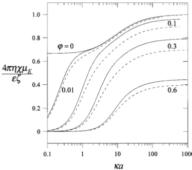
In Fig. 2, the numerical results for the dimensionless elec-trophoretic mobility 4πηχµE/εζ for a suspension of charged spheres calculated from Eq. [32] incorporating with Eqs. [28]
FIG. 2. Plots of the dimensionless electrophoretic mobility 4πηχµE/εζ in a suspension of identical spheres versusκa with ϕ as a parameter. The solid and dashed curves represent the calculations for the Happel and Kuwabara cell models, respectively.
and [31b] are plotted versusκa with ϕ as a parameter for both the Happel and Kuwabara models. In this figure, the coefficient χ is included in the mobility definition to eliminate the effect of the boundary condition for the electric potential prescribed at the virtual surface of the unit cell. It can be seen that this dimension-less mobility is a monotonic decreasing function ofϕ for a given value ofκa. Also, for a fixed value of ϕ, the particle mobility de-creases monotonically with a decrease inκa (or with an increase in the double-layer overlap). Whenκa = 0, µE= εζ/6πη as ϕ = 0 and µE= 0 for all finite values of ϕ. Thus, when the double layers are thick (say,κa ≤ 0.2), the particle concentra-tion effect on the electrophoretic mobility is significant even in fairly dilute suspensions. For concentrated suspensions, this ef-fect is evident for even relatively thin double layers. Figure 2 illustrates that, for any combination ofκa and ϕ, the Kuwabara model predicts a smaller value (or a stronger particle concentra-tion dependence) for the electrophoretic mobility than the Hap-pel model does. This occurs because the zero-vorticity model yields a larger energy dissipation in the cell than that due to particle drag alone, owing to the additional work done by the stresses at the outer boundary (12).
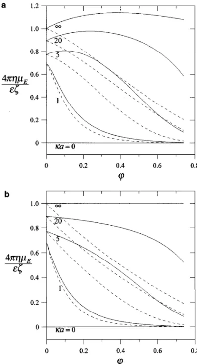
The results for the normalized electrophoretic mobility 4πηµE/εζ for a suspension of spherical particles are plotted as a function ofϕ in Fig. 3 for various values of κa. The calcu-lations are presented up toϕ = 0.74, which corresponds to the maximum attainable volume fraction for a swarm of identical spheres (15). When the boundary condition [7a] or [14] for the electric potential at the virtual surface of the cell is used, the nor-malized mobility is a monotonic decreasing function ofϕ for a given finite value ofκa (and equals unity as κa → ∞, regardless of the value ofϕ) for the case of the Kuwabara model. However, for the case of the Happel model, the particle mobility is not a monotonic function ofϕ and has a maximum for a fixed value ofκa greater than about unity. The location of this maximum shifts to greaterϕ as κa increases. For a constant value of κa less than about unity, this mobility is still a monotonic decreasing function ofϕ. On the other hand, when the boundary condition [15] or [16] for the electric potential at the outer surface of the cell is used, both the Happel and Kuwabara models predict that the electrophoretic mobility decreases monotonically with an in-crease inϕ for a given value of κa. For an arbitrary combination ofκa and ϕ, the value of the electrophoretic mobility calculated using the boundary condition [14] is always greater than that calculated using the boundary condition [16].
In theoretical studies based on the reflection solution of inter-actions between pairs of electrophoretic spheres together with the concepts of statistical mechanics (26) and on the multipole-expansion solution of electrokinetic properties in a cubic cell filled with randomly placed spheres (27) as well as in an experimental investigation on the electrophoresis of human ery-throcytes (25), it has been found that the mean electrophoretic mobility in a bounded (dilute or concentrated) suspension of identical spheres withκa ≥ 20 decreases monotonically with an increase inϕ. Thus, the boundary condition [14] for the cell
FIG. 3. Plots of the normalized electrophoretic mobility 4πηµE/εζ in a suspension of identical spheres versusϕ with κa as a parameter: (a) the Happel model and (b) the Kuwabara model. The solid and dashed curves represent the calculations using the boundary conditions [14] and [16], respectively.
model is not as accurate as the boundary condition [16] in com-parison with these theoretical results and experimental data. This outcome is probably due to the fact that the angular component of the potential gradient at the outer boundary of the cell is not specified in Eq. [7a] or [14]. In Fig. 4, a comparison between some experimental data of the normalized electrophoretic mo-bility 4πηµE/εζ for bounded suspensions of identical spheres withκa → ∞ as a function of ϕ (25) and our results of Eq. [49] for the Happel and Kuwabara models using the boundary condi-tion [15] or [16] for the electric potential at the virtual surface of the cell is provided. Some other relevant theoretical predictions (22–24, 27) are also plotted in this figure for comparison. It can
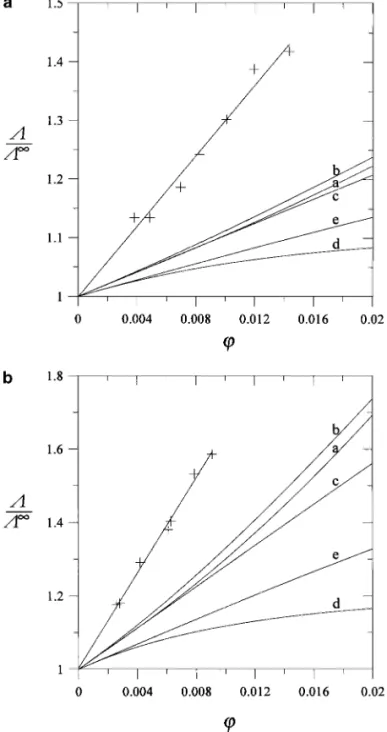
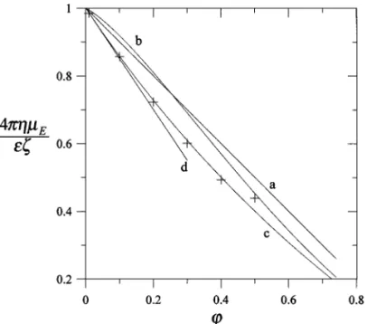
FIG. 4. Comparisons of the normalized electrophoretic mobility 4πηµE/εζ in bounded suspensions of identical spheres withκa → ∞ as a function of ϕ. Curve a represents experimental data for human erythrocytes, 4πηµE/εζ ≈ 1− ϕ (25). Curves b and c represent our results of Eq. [49] for the Hap-pel and Kuwabara models, respectively, using the boundary condition [16]. Curve d denotes the prediction from statistical mechanics, 4πηµE/εζ = 1 − (3/2)ϕ + O(ϕ2) (22–24). The points are numerical results obtained by Kang and Sangani (27).
be seen that the prediction from the Happel model agrees quite well with the experimental data, while the result of the Kuwabara model differs little from the other theoretical predictions.
The dimensionless coefficient H2I of the O(ζ ) term in
Eq. [41] for the effective conductivity of a suspension of iden-tical charged spheres is plotted in Fig. 5 as a function of the parametersκa and ϕ. It can be seen that the coefficient H2I is always a negative value and thus the presence of the particle charges reduces the magnitude of the effective conductivity for any volume fraction of particles in the suspension if the product ofβ and ζ is positive and increases this magnitude if βζ < 0. For a given value ofκa the effect of the particle charges on the effec-tive conductivity is maximal at some value ofϕ and vanishes as ϕ = 0. The location of the maximum in −H2I shifts to greaterϕ asκa increases. On the other hand, for a fixed value of ϕ, −H2I
is a monotonic decreasing function ofκa and approaches zero asκa → ∞. When ϕ is not too large (≤0.5), the value of −H2I
calculated using the boundary condition [14] is always greater than that calculated using the boundary condition [16].
The dimensionless coefficient H2J1of the O(ζ2) term in Eq. [41] is plotted in Fig. 6 for various values ofκa and ϕ. Unlike the coefficient H2I (and H2J
2), the value of H2J1depends on the boundary condition for the fluid velocity at the virtual surface of the unit cell. It can be found that the value of H2J
1predicted by the Happel model is larger than that predicted by the Kuwabara model, but in general, the difference is small. For a specific value ofκa, H2J
1is not a monotonic function ofϕ and has a maximal
value. The location of this maximum shifts to greaterϕ as κa increases. Also, for a constant value ofϕ, a maximum of the coefficient H2J
1 would appear. Asϕ increases, the maximum occurs at largerκa. In the limit of ϕ = 0 or κa → ∞, H2J
1= 0. Figure 7 shows plots of the dimensionless coefficient H2J
2 of the O(ζ2) term in Eq. [41] for various values ofκa and ϕ. In general, the trend of the dependence of H2J2onκa and ϕ is quite similer to that for H2I , but the magnitude of H2J2is smaller. Depending on the combination ofκa and ϕ, the value of H2J2 calculated using the boundary condition [14] can be either greater or smaller than that calculated using the boundary condition [16].
FIG. 5. Plots of the dimensionless coefficient H2I in Eq. [41] for the electric conductivity of a suspension of identical spheres versus the parameters κa and ϕ. The solid and dashed curves represent the calculations using the boundary conditions [14] and [16], respectively.
FIG. 6. Plots of the dimensionless coefficient H2J
1 in Eq. [41] for the electric conductivity of a suspension of identical spheres versus the parameters κa and ϕ: (a) the Happel model and (b) the Kuwabara model. The solid and dashed curves represent the calculations using the boundary conditions [14] and [16], respectively.
Watillon and Stone-Masui (8) have measured the electric conductivities of suspensions of polystyrene latex spheres with various values of diameter and zeta potential. Few of their ex-periments are suitable for comparison with the theory devel-oped here which requires the assumptions of a single symmetric electrolyte [correct to O(ζ2)] and a low zeta potential. Nonethe-less, the results of two of these experiments, (a) a suspension of 70-nm-diameter spheres with a zeta potential of−62.2 mV in the presence of 0.1 mM HClO4 (κa = 1.13) and (b) a suspen-sion of 56-nm-diameter spheres with a zeta potential of−99 mV in 0.1 mM HCIO4(κa = 0.91), are compared with our Happel model predictions of Eqs. [41]–[44] for the effective
conductiv-ity in Fig. 8. The results of the normalized conductivconductiv-ity3/3∞ for the Kuwabara model are not shown in this figure because their numerical differences from the corresponding results for the Happel model are quite small (and negative). The theoret-ical predictions made by O’Brien (7) correct to O(ζ2) for a dilute suspension and by Ohshima (20) correct to O(ζ) using the Kuwabara cell model and boundary condition [14] without consideration of the overlap of the adjacent double layers on the virtual surface of the cell are also exhibited in this figure for com-parison. It can be seen that all of these theoretical analyses under-predict the experimental results. (In contrast, a recent numerical calculation involving a finite-difference method for the electric conductivities of these two suspensions based on the Kuwabara
FIG. 7. Plots of the dimensionless coefficient H2J
2 in Eq. [41] for the electric conductivity of a suspension of identical spheres versus the parameters κa and ϕ. The solid and dashed curves represent the calculations using the boundary conditions [14] and [16], respectively.
FIG. 8. Comparisons of the normalized electric conductivity3/3∞as a function ofϕ: (a) a suspension of 70-nm-diameter spheres having a zeta poten-tial of−62.2 mV in 0.1 mM HClO4and (b) a suspension of 56-nm-diameter spheres with a zeta potential of−99 mV in 0.1 mM HClO4. The points were measured by Watillon and Stone-Masui (8). Curves a and b represent our re-sults of Eq. [41] for the Happel model using the boundary conditions [14] and [16], respectively. Curves c and d represent the predictions of O’Brien (7) and Ohshima (20), respectively. Curve e denotes our result of the Kuwabara model using the boundary condition [14] correct to O(ζ) only.
cell model and boundary condition [14] neglecting the relaxation effect (18) overpredicts the experimental results.) When the con-tribution of the O(ζ2) term is included, our results are closer to the experimental data than O’Brien’s analysis is, presumably be-cause we have considered the effect of particle interactions in the suspension. Note that the particle interaction effect on the effec-tive conductivity determined by using the boundary condition [16] is stronger than that calculated using the boundary
condi-tion [14]. Again, condicondi-tion [14] is less accurate than condicondi-tion [16] for the cell model in comparison with the experimental data. In the previous cell-model analyses for the electric conductiv-ity of a suspension of charged particles, it was assumed that the overlap of the electric double layers of adjacent particles could be neglected (16, 18, 20). It would be of interest to know whether this assumption is valid in typical situations. In Fig. 8, our cal-culations of3/3∞relaxing this assumption and corresponding to Ohshima’s analysis (correct to O(ζ) using the Kuwabara cell model and boundary condition [14]) are also presented for a comparison. It can be seen that the analysis with nonoverlap-ping double layers underestimates the conductivities of the two suspensions withκa in the order of unity; the errors increase with the volume fraction of the particles and can be meaningful. Comparison between curves a and e in Fig. 8 also indicates that the errors in the effective conductivity owing to neglect of the
O(ζ2) contribution are quite significant.
6. SUMMARY
In this paper, the steady-state electrophoresis in a homoge-neous suspension of identical charged spheres in an electrolyte solution with an arbitrary value ofκa is analyzed by employing the Happel and Kuwabara cell models. Solving the linearized electrokinetic equations applicable to the system of a sphere in a unit cell by a regular perturbation method, we have obtained the electrochemical potential energies of the electrolyte ions and the fluid flow field. The requirement that the total force exerted on the unit cell is zero leads to Eq. [28] or [32] for the elec-trophoretic mobility of the charged sphere correct to the orderσ orζ. It is found that, with the use of the Debye–H¨uckel approxi-mation, the normalized electrophoretic mobility is a monotonic increasing function of κa for constant values of the volume fraction of particles. Based on the solution for the fluid velocity and electrochemical potentials in a unit cell, an explicit formula, Eq. [41], for the effective conductivity of the suspension is ob-tained as a power series in the zeta potential of the particles up to
O(ζ2). According to this formula, the particle charges can result in an increase or a decrease in the effective conductivity relative to that of a corresponding suspension of uncharged particles, depending on the diffusion coefficients of the electrolyte ions and the sign of the particle charges. Our results show that the previous analyses for the electric conductivity of suspensions of charged particles with nonoverlapping double layers can be in significant error in typical situations. Comparisons of the results of the electrophoretic mobility and the effective conductivity be-tween the Happel model and the Kuwabara model with different conditions for the electric potential at the outer boundary of the cell have been provided.
Equations [32] and [41] with Eqs. [28] and [42]–[44] are de-rived on the basis of the Debye–H¨uckel approximation for the equilibrium potential distribution around the dielectric sphere in a unit cell. The reduced formulas of Eqs. [42]–[44] for the electric conductivity of a dilute suspension of identical charged spheres with low zeta potential, Eqs. [46]–[48], were shown
to give a good approximation for the case of reasonably high zeta potential (with an error of about 5% in a KCl solution and less than 2% in a HClO4solution for the case ofζ e/kT = −2) (7). Also, comparing with the numerical solution for the elec-trophoretic mobility of a charged sphere in KCl solutions ob-tained by O’Brien and White (3) valid for an arbitrary value of zeta potential, one can find that formula [45] for a dilute suspension of dielectric spheres with low zeta potential is also quite accurate for reasonably high zeta potentials (with errors less than 4% forζ e/kT ≤ 2). Therefore, our results for Eqs. [32] and [41] might be used tentatively for the situation of reasonably high electric potential. In order to see whether our approximate solution can be extended to the higher values of electric poten-tial, a numerical solution of the electrokinetic equations with no assumption on the magnitude of electric potential would be needed to compare it with the approximate solution.
APPENDIX
The functions F1r(r ), F1θ(r ), Fp1(r ), and Fm1(r ) in Eqs. [26]
and [27] are listed here:
F1r(r )= C1+ C2 µ a r ¶ + C3 µ a r ¶3 + C4 µ r a ¶2 + Z r a µ r a ¶2 G(r ) dr− µ a r ¶ Z r a µ r a ¶3 G(r ) dr +1 5 µ a r ¶3Z r a µ r a ¶5 G(r ) dr−1 5 µ r a ¶2Z r a G(r ) dr, [A1a] F1θ(r )= −C1− C2 2 µ a r ¶ +C3 2 µ a r ¶3 − 2C4 µ r a ¶2 − Z r a µ r a ¶2 G(r ) dr+ µ a 2r ¶ Z r a µ r a ¶3 G(r ) dr + 1 10 µ a r ¶3Z r a µ r a ¶5 G(r ) dr+2 5 µ r a ¶2Z r a G(r ) dr, [A1b] Fp1(r )= C2 µ a r ¶2 + 10C4 µ r a ¶ − µ a r ¶2Z r a µ r a ¶3 G(r ) dr − 2 µ r a ¶ Z r a G(r ) dr, [A1c] Fm1(r )= z2 me2 3kT (1− ϕ) ½ a3A µ1(a, b) + 2ϕBµ1(a, b) 2(1− ϕ)r2 + · ϕ Aµ1(a, b)+b23Bµ1(a, b) ¸ r 1− ϕ+ 1 r2Bµ1(a, r) + r Aµ1(r, b) ¾
(when Eq. [25d] or [14] is used), [A2a] Fm1(r )= z2 me2 3kT [1+ (1/2)ϕ] ½ a3A µ1(a, b) − ϕBµ1(a, b) (2+ ϕ)r2 − · ϕ Aµ1(a, b)+b23Bµ1(a, b) ¸ r 2+ ϕ+ 1 r2Bµ1(a, r) + r Aµ1(r, b) ¾
(when Eq. [25e] or [16] is used), [A2b] where G(r )= − εκ 2a2 24πηχ · 2+ µ a r ¶3¸ dψeq1 dr , [A3] Aµ1(x, y) = Z y x µ 1−a 3 r3 ¶ dψeq1 dr dr, [A4a] Bµ1(x, y) = Z y x µ r3− a3 ¶ dψeq1 dr dr. [A4b]
Note that, for a symmetrically charged electrolyte, F+1= F−1. The constants Ciwith i =1, 2, 3, and 4 in Eq. [A1] are
C1= − ·µ 1+3 2ϕ 5/3 ¶ A1+ 5 2ϕB1 ¸ ω, [A5a] C2= ·µ 3 2+ ϕ 5/3 ¶ A1+ 5 2ϕ 2/3B 1 ¸ ω, [A5b] C3= − · 1 2A1+ µ 3 2ϕ 2/3− ϕ ¶ B1 ¸ ω, [A5c] C4= · 1 2ϕ 5/3A 1− µ ϕ2/3−3 2ϕ ¶ B1 ¸ ω, [A5d] A1= µE1+ Z b a µ r a ¶2 G(r ) dr− µ a b ¶ Z b a µ r a ¶3 G(r ) dr, [A6a] B1= 1 5 µ a b ¶3Z b a µ r a ¶5 G(r ) dr −1 5 µ b a ¶2Z b a G(r ) dr, [A6b]
for the Happel model, and
C1= − ·µ 1+1 2ϕ ¶ A01+ µ 1−5 2ϕ + 3 2ϕ 5/3 ¶ B10 ¸ ω0, [A7a] C2= · 3 2A 0 1+ µ 3 2− 5 2ϕ 2/3+ ϕ5/3 ¶ B10 ¸ ω0, [A7b]
C3= − ·µ 1 2 − 1 5ϕ ¶ A01+ µ 1 2− 3 2ϕ 2/3+ ϕ ¶ B10 ¸ ω0, [A7c] C4= · 3 10ϕ A 0 1+ µ ϕ2/3−3 2ϕ + 1 2ϕ 5/3 ¶ B10 ¸ ω0, [A7d] A01= µE1+ Z b a µ r a ¶2 G(r ) dr− µ a b ¶ Z b a µ r a ¶3 G(r ) dr +1 5 µ a b ¶3Z b a µ r a ¶5 G(r ) dr−1 5 µ b a ¶2Z b a G(r ) dr, [A8a] B10 = −1 5 µ a b ¶ Z b a µ r a ¶3 G(r ) dr+1 5 µ b a ¶2Z b a G(r ) dr, [A8b]
for the Kuwabara model, where ω = µ 1−3 2ϕ 1/3+3 2ϕ 5/3− ϕ2 ¶−1 , [A9a] ω0= µ 1−9 5ϕ 1/3+ ϕ −1 5ϕ 2 ¶−1 · [A9b]
The functions F±2(r ) in Eq. [30] are listed here:
F±2(r )= ∓ Z e 3kT ½ a3A ±2(a, b) + 2ϕB±2(a, b) 2(1− ϕ)r2 + · ϕ A±2(a, b) + 2 b3B±2(a, b) ¸ r 1− ϕ + 1 r2B±2(a, r) + r A±2(r, b) ¾
(when Eq. [14] is used), [A10a]
F±2(r )= ∓ Z e 3kT ½ a3A ±2(a, b) − ϕB±2(a, b) (2+ ϕ)r2 − · ϕ A±2(a, b) + 2 b3B±2(a, b) ¸ r 2+ ϕ + 1 r2B±2(a, r) + r A±2(r, b) ¾
(when Eq. [16] is used), [A10b]
where A±2(x, y) = Z y x · d F±1 dr − kT D±F1r(r ) ¸ dψeq1 dr dr, [A11a] B±2(x, y) = Z y x r3 · d F±1 dr − kT D±F1r(r ) ¸ dψeq1 dr dr, [A11b]
and the functions ψeq1(r ), F1r(r ), and F±1(r ) are given by Eqs. [18], [Ala], and [A2], respectively.
ACKNOWLEDGMENTS
This research was partially supported by the National Science Council of the Republic of China.
REFERENCES
1. Henry, D. C., Proc. R. Soc. London, Ser. A 133, 106 (1931). 2. Booth, F., Proc. R. Soc. London, Ser. A 203, 514 (1950).
3. O’Brien, R. W., and White, L. R., J. Chem. Soc., Faraday Trans. 2 74, 1607 (1978).
4. Wiersema, P. H., Loeb, A. L., and Overbeek, J. Th. G., J. Colloid Interface Sci. 22, 78 (1966).
5. Dukhin, S. S., and Derjaguin, B. V., in “Surface and Colloid Science” (E. Matijevic, Ed.), Vol. 7, Wiley, New York, 1974.
6. Saville, D. A., J. Colloid Interface Sci. 71, 477 (1979). 7. O’Brien, R. W., J. Colloid Interface Sci. 81, 234 (1981).
8. Watillon, A., and Stone-Masui, J., J. Electroanal. Chem. 37, 143 (1972).
9. Ohshima, H., Healy, T. W., and White, L. R., J. Chem. Soc., Faraday Trans. 2 79, 1613 (1983).
10. Liu, Y. C., and Keh, H. J., J. Colloid Interface Sci. 192, 375 (1997).
11. Liu, Y. C., and Keh, H. J., Langmuir 14, 1560 (1998).
12. Happel, J., and Brenner, H., “Low Reynolds Number Hydrodynamics,” Nijhoff, The Netherlands, 1983.
13. Happel, J., AIChE J. 4, 197 (1958).
14. Kuwabara, S., J. Phys. Soc. Jpn. 14, 527 (1959).
15. Levine, S., and Neale, G. H., J. Colloid Interface Sci. 47, 520 (1974).
16. Kozak, M. W., and Davis, E. J., J. Colloid Interface Sci. 127, 497 (1989).
17. Kozak, M. W., and Davis, E. J., J. Colloid Interface Sci. 129, 166 (1989).
18. Johnson, T. J., and Davis, E. J., J. Colloid Interface Sci. 215, 397 (1999).
19. Ohshima, H., J. Colloid Interface Sci. 188, 481 (1997). 20. Ohshima, H., J. Colloid Interface Sci. 212, 443 (1999).
21. Lee, E., Chu, J., and Hsu, J., J. Colloid Interface Sci. 209, 240 (1999).
22. Anderson, J. L., Ann. N. Y. Acad. Sci. 469 (Biochem. Eng. 4), 166 (1986).
23. Chen, S. B., and Keh, H. J., AIChE J. 34, 1075 (1988).
24. Acrivos, A., Jeffrey, D. J., and Saville, D. A., J. Fluid Mech. 212, 95 (1990).
25. Zukoski, C. F., and Saville, D. A., J. Colloid Interface Sci. 115, 422 (1987).
26. Tu, H. J., and Keh, H. J., J. Colloid Interface Sci. 231, 265 (2000). 27. Kang, S., and Sangani, A. S., J. Colloid Interface Sci. 165, 195
![FIG. 7. Plots of the dimensionless coefficient H 2 J 2 in Eq. [41] for the electric conductivity of a suspension of identical spheres versus the parameters κa and ϕ](https://thumb-ap.123doks.com/thumbv2/9libinfo/8868615.247127/11.918.483.876.353.1083/dimensionless-coefficient-electric-conductivity-suspension-identical-spheres-parameters.webp)