The Algorithms for Resource Management in Next Generation Wireless Network
17
0
0
全文
(2) 1 Introduction In UMTS, applications and services can be divided into four traffic classes. These traffic classes have been classified into real-time classes and non-real-time classes [1]. The known traffic classes for the real-time are conversational and streaming applications, and interactive and background classes are dealt with as non-real-time applications. In particular, the real-time conversational traffic is the most delay-sensitive class. The Wideband Code Division Multiple Access (WCDMA) is an air interface for UMTS, which adopts code division technology to increase spectral efficiency and enhance the system's capacity. To be a successful system, WCDMA has to support Quality of Service (QoS) requirements for real-time applications. In the standard 3GPP Release 5, UMTS has emerged as IP multimedia architecture [2]. The architecture enables session initial protocol (SIP)-based call control of packet-oriented connections, to offer voice over IP (VoIP) and video telephony services. IP-based network entities integrated voice and data on unified IP backbone, which can increase the resource utilization over existing mobile networks. Next generation WCDMA must manipulate the delay-sensitive real-time packets to provide IP multimedia service. The resource management of the radio access network will become the most important issue for real-time packets quality-of-service (QoS) provisioning because of the scarcity of radio frequencies. Several researchers have recently proposed the concept of IP-based radio access networks to utilize efficiently radio resources [3]. In an IP-based radio access network, the real-time traffics are transmitted as packet-oriented connections over an air interface. Therefore, applying the radio access architecture will benefit radio resource utilization for multimedia services. Several resource management polices have been proposed to improve radio resource utilization [4]-[6]. With the help of power assignment and code hopping, Gürbüz and Owen [4] proposed a resource scheduler in the base station that collected requests from all mobile users. The real-time traffic in a radio access network can have priority serving and higher bit rate than non-real-time traffic. Jorguseski et al. [5] proposed a resource allocation algorithm, which considered the session bit rate to determine the transmission power that could fit the Eb/No target ranges, by iteratively using the power control process. Most literature considers real-time problems, which solve the congestion control of the switching element and allocated resources for the multi-processor, using real-time packet scheduling algorithms [7][8]. In this paper we describe two real-time packet scheduling scheme in next generation WCDMA for QoS provisioning. The rest of the 2.
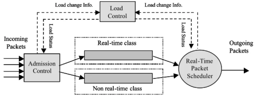
(3) paper is organized as follows. In section 2, a generic framework for packet QoS provisioning is defined. In section 3, two real-time algorithms for packet scheduling are presented. In section 4 we present simulation results to demonstrate the performance of our packet scheduling algorithms. Concluding remarks are given in section 5.. 2 Radio resource allocation of packet access In a WCDMA system, the available channelization codes and base station power are the most important resources [9]. In this section, a generic management framework is described within the radio access network to schedule real-time packet traffic for resource utilization. Figure 1 illustrates the management framework implemented at radio access network. The Admission Control (AC), based on the system resource, decides whether a new data session is accepted by the access system. When a data session is accepted, AC classifies packet traffic into real-time queue and non real-time queue. The resource allocation is allowed if the estimated power consumption does not exceed a target threshold. If an overload situation occurs, Load Control (LC) will execute the overload control that invokes either AC to drop a call or PS to decrease the transmitted bit rate for reducing the power consumption. The function of PS is to schedule the allocated radio frequency resource and ensure availability of air interface capacity for all real-time packet traffic.. Load change Info.. Load Status. Load Status. Incoming Packets. Load change Info.. Load Control. Real-time class. Outgoing Packets. Real-Time Packet Scheduler. Admission Control Non real-time class. Figure 1 A generic framework for real-time traffic in radio access network.. Let txmax be the maximum transmission power of a base station, and txadmit is the threshold for admitting new real-time session. In the beginning, AC decides whether the allocated power of a base station is larger than txadmit . If the allocated power is 3.
(4) smaller than the value of txadmit , the AC allows establishment of the real-time data session and then invokes PS to allocate radio resources to the data session. If the allocated power is larger than txadmit , then AC rejects the request. The allocated power is increased to overcome mobile user increment and degeneration of circumstances. When the power consumption exceeds txadmit , LC must ask PS to execute the real-time scheduling algorithm to reschedule the traffic. In a WCDMA system, many subscribers simultaneously use the same frequency. The WCDMA uses channelization codes to spread information for each mobile user based on the orthogonal variable spreading factor (OVSF) technique. Different users employ different channelization codes for packet transmission. The channelization code is assigned according to the user-required bit rate and service QoS. The simultaneous use of the same frequency by many users makes interference between the users likely. In the case of much interference, the base station must increase power of transmission to ensure mobile users receive data correctly.An air interface model is applied to analyze the interference of WCDMA and illustrate the power consumption. Based on the capacity analysis model [10], the base station output power can be written as, n. Ptot =. [1 + n ⋅ r ⋅ (1 − β )] + PSCH + PCCH + ∑ r ⋅ GNk 1 − n ⋅ r ⋅ (β + λ). k =1. (1). Assume that a base station current serves n mobile users. PSCH is the transmitting power of the non-orthogonal synchronization channel; PCCH is the transmitting power of the orthogonal common control channel, and N is a floor noise parameter. Suppose that a base station transmits power for dedicated channels and common channels that have a β percent loss of their orthogonality, and λ is the rate of power reception from intra-cell to inter-cell. Gk denotes the path gain from the base station to mobile user k, and r denotes the SIR.. Table 1 Bit rate (K bps) Eb N0. (db). r (SIR). Values of. Eb N0. and r with different bit rates.. 8. 16. 32. 64. 128. 256. 512. 4.2. 3.2. 2.8. 2.4. 2.3. 2.2. 2.1. 0.0103. 0.0163. 0.2074. 0.4055. 0.0301 0.0543 0.1061. 4.
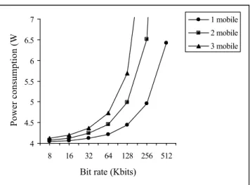
(5) 1 mobile. Power consumption (W). 7. 2 mobile. 6.5. 3 mobile. 6 5.5 5 4.5 4 8. 16. 32. 64. 128 256 512. Bit rate (Kbits). Figure 2 Power consumption of mobile with different bit rate.. Table 1 shows. Eb N0. with different bit rates for a mobile speed of 3 km/h and an. FER target of 10% [11]. Evaluating the power consumption of the base station, the values of the corresponding parameters are defined as [10], n:1 PSCH : 0.2 W PCCH : 3.8 W N : - 99 dbm. β : 0.06 λ : 0.84. Gk : 0.2, where k = 1,… ,n Figure 2 illustrates the simulation results of the base station power consumption for various input parameters. In Fig. 2, the power consumption of the base station is increased with the both allocated bit rate and the number of active mobiles. Hence, the base station power consumption can decrease by reducing the number of active mobiles and the bit rate allocation in a cell. Moreover, via the previous analysis, preventing the simultaneous use of many active mobiles within a cell is advantageous.. 3 Real-time scheduling schemes Recall that the real-time packet services are periodic multimedia traffic, such as 5.
(6) VoIP, video conferencing and video streaming. In a mobile system, the following hypotheses are assumed to apply to the real-time packet services. For each service request, the mobile system creates a new data session and a QoS profile according to the service class. Each data session contains many tasks. For real-time tasks, the arrival rate is constant. A real-time task can be active for transmission when it arrives. The time interval between two active real-time tasks is the period. The mobile system defines a deadline for each real-time task according to the QoS profile. The relative deadline is equal to the period of the real-time task. Moreover, the non real-time tasks will be scheduled after setting enough radio resource for all the arrived real-time tasks to complete on time. In particular, each active task must be assigned an appropriate channelization code that depends on the required bit rate and the maximum bit rate of the QoS profile. The Generic scheduling algorithm applies the functionalities AC, PS and LC for real-time packet QoS provisioning. Parameter txadmit determines the power threshold for newly admitted real-time data sessions, based on the capacity analysis model of Eq. (1). If a data session request arrives, the management framework defines the instance’s period, processing time, required bit rate and allowed maximum bit rate, according to the QoS profile of service. The Generic scheduling algorithm works as follows. 1.. In the beginning, the PS maintains a prioritized queue in which instances of data sessions are ordered on a first-in-first-out (FIFO) basis.. 2.. When a data session request arrives, the AC reserves power according to the required bit rate. The LC estimates the power consumption using the capacity analysis model.. 3.. The AC decides whether the power, Ptot, exceeds the threshold, txadmit, or not. If the power, Ptot, is smaller than the threshold, txadmit, a new data session is admitted. Otherwise, the AC rejects the request.. 4.. If a new data session is established, the PS puts the session’s instance into the queue, and schedules the instances of the queue for execution. The PS, based on the required bit rate, assigns the channization code and required power for the instance. After the power allocation is finished, the PS asks the LC to change the system’s load.. 5.. The PS terminates an instance when it is finished or when its deadline is reached. When an instance is terminated, the PS removes this instance from the queue and releases the occupied channelization code and the allocated power. Finally, the PS asks the LC to change the system’s load. 6.
(7) For packet transmission, we propose two packet scheduling schemes to reduce power consumption based on the capacity analysis model. The algorithms can prevent large packets from being simultaneously transmitted (high packet activities at the same time), based on the tolerance of service delay, and can thus decrease active mobile users.. A. Real-time bandwidth scheduling The real-time bandwidth scheduling (RTBS) algorithm applies the functionalities AC, PS and LC for real-time packet QoS provisioning. Parameter txadmit is determined the power threshold for newly admitted real-time data sessions, based on the capacity analysis model of Eq. (1). Using the EDF scheme, the RTBS makes the schedulable analysis that schedules the real-time data sessions for saving power resource. Due to the delay constraint, all tasks of a data session are delivered in time to meet their deadline. If a task completes transmission before its deadline, the RTBS could defer the task active time (but not miss the task’s deadline). Since tasks can be deferred, the base station will control code and power allocations and prevent large mobile user activities at the same time. Now, let us consider that whether a data session is a feasible schedule by using EDF scheme. The RTBS makes schedulable analysis that is based on the task period time and process time of a data session, and the allocated channel number C of a base station. Assuming that P i denotes task i process time by using one channelization code. C denotes the amount of channelization codes that is allowed allocating by a base station. If a channelization code is used to spread a task, the system can create C channelization codes for spreading C tasks simultaneously with the available power resource; therefore, Pi C denotes the task i process time that uses C channelization codes to spread it simultaneously. Since E i denotes the task i period,. Pi. C. is the. Ei. fraction of radio resource that is spent on transmitting task i. Then, the resource utilization for n active tasks is given by n. Pi. i. Ei. U =∑. C. Based on the schedulable analysis, a set of periodic tasks is schedulable with EDF in a base station if and only if the resource utilization U is less than 1. Thus, if U ≤ 1 , task i is a feasible schedule by EDF scheme. We can defer to active task i before the task misses its deadline. On the other hand, if U > 1 , task i is not a feasible schedule by 7.
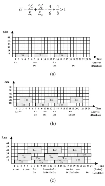
(8) EDF scheme. Then, a new channelization code must immediately allocate for the session to manipulate the session schedulability. For a data session request, the management framework defines task’s period time E, process time P, initiated bit rate Ri and allowed maximum bit rate Rmax according to the QoS profile of service. The RTBS works as follows: 1.. In the beginning, the PS maintains a prioritized task queue in which tasks are ordered according to the EDF basis. The PS makes schedulable analysis for the session when a data session request arrives. The utilization factor, U, is calculated using the task’s period time E, process time P and the presently assigned channel number C.. 2.. If U ≤ 1 , the data session is a feasible schedule by EDF. The AC allows for the session establishment. Go to Step 5. If U > 1 , the data session is not a feasible schedule by EDF. The PS increases the channel number, C. The LC makes power reservation to increase channel number. According to the required bit rate, the LC estimates power consumption Ptot of the base station. If the power, Ptot, is below the threshold txadmit , then a new session is admitted. Otherwise, the AC rejects the request.. 3.. If a data session is admitted, the PS puts session’s task into the task queue and schedules it. The scheduler chooses the first C tasks (early deadline tasks) in the task queue for execution. The lower priority tasks (late deadline tasks) will be deferred. The PS, based on the required bit rate, assigns the channelization code and the required power for the tasks. Following the power allocation, the PS asks the LC to change the system’s load.. 4.. The PS terminates a task when it is completed or its deadline is reached. When a task is terminated, the PS removes this task from the task queue and releases the occupied channelization code as well as the allocated power. Finally, the PS asks the LC to change the system’s load.. Figure 3 illustrates a feasible schedule constructed using the RTBS. Based on the service profiles (Table 2), the figure shows the schedule of four sessions at time t = 24. In Fig. 3(a), task T11 of session J1 arrives at time t=1. The task’s required bit rate, R1, is 8K. The channelization code of a 8 K bit rate is assigned to J1, and sets the channel number C=1. Tasks T11, T12 and T13 are schedulable before their deadlines (Fig. 3(a)). In Fig. 3(b), task T21 of session J2 arrives at time t=2 and requires a bit rate of R2=16 K. Consider the channel number C =1, for which the utilization factor, U, is, 8.
(9) U=. P1. C. E1. +. P2. =. C. E2. 4 4 + >1 6 8. Rate 6R 5R 4R 3R 2R 1R. T 11. T 12. T 13 Time. 1 2 3 4 5 6 7 8 9 10 11 12 13 14 15 16 17 18 19 20 21 22 23 24 A 11. A 12. A 13. D 11. D12. (Arrive) (Deadline). D13. (a) Rate 6R 5R 4R 3R 2R 1R. T 21. T 22. T 11. T 23. T 12. T 13 Time. 1 2 3 4 5 6 7 8 9 10 11 12 13 14 15 16 17 18 19 20 21 22 23 24 A 11 A21. A 12. A 22. A 13. A 23. D11. D21. D12. D22 D13. (Arrive) (Deadline). (b) Rate 6R 5R 4R 3R 2R 1R. T41 T 21 T 11. T42 T22. T 31 T 12. T43 T 32. T 13. T33 T23. 1 2 3 4 5 6 7 8 9 10 11 12 13 14 15 16 17 18 19 20 21 22 23 24 A 11 A 21. A 31A 41. A 12. A 22 A 42A 32A 13. A 43 A 23. A 33. D 11. D21 D41 D31 D 12. D42 D22 D13 D 32. D43. Time (Arrive) (Deadline). (c) Figure 3 An example illustrating the usage of RTBS algorithm.. Table 2. Selected input parameters.. Session Arrival Period Process Initiated Maximum (Ji) Time (Ai) Time (Ei) Time (Pi) Rate: Rate: Kbps (Ri) Kbps (Rmax) J1 J2 J3 J4. 1 2 4 5. 6 8 8 6. 4 4 4 4 9. 8 16 8 16. 16 32 16 32.
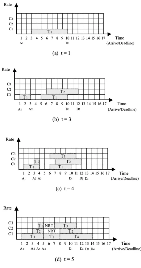
(10) J2 is not a feasible schedule by the EDF scheme since U > 1 . That is, all tasks of J2 cannot complete transmission with channel number C=1. In this case, PS assigns another new channelization code whose bit rate is 16 K for S2, and then sets the channel number C=2. Then,. U=. P1. C. E1. +. P2. 2 2 = + <1 E2 6 8 C. Tasks T21, T 22 and T23 can be scheduled before their deadlines (Fig. 3(b)). Similarly, RTBS can use two channelization codes to schedule sessions J1 – J3 (Fig. 3(c)). In this case, RTBS only applies three channelization codes to control four real-time data sessions, in which the amount of the bit rate allocation is 40K (at time t=13), and the maximum power consumption is 4.17W.. B. Real-time imprecise scheduling In this section, we concentrate on real-time imprecise scheduling (RTIS) algorithm to improve radio resource utilization. The RTIS is constructed using the reverse scheduling approach to schedule aperiodic real-time tasks. The real-time tasks are scheduled from the latest deadline backwards to the current time. Each task is scheduled at or before its deadline, and tasks are scheduled in the latest-ready-time-first-order. For a data session request arrives, the task’s ready time A, process time P, and deadline D are defined according to the QoS profile of service. To speed up the algorithm, we keep on the available time for each allocated resource on a reservation array Favail other than the reservation time of executing tasks [12]. In particular, the reservation element, Favail(C), for executing task Ti is given by Favail (C ) = (Di − t ) −. ∑ (P. j T j ∈C & D j ≤ Di. −Ej). (2). where Tj is a task that is scheduled by rate code C. P j and E j are respective the process time and completed time of Tj at the time t. Notably, task Ti cannot be scheduled by rate code C when Favail(C) < 0. In this case, the system must allocate a new rate code for Ti. The RTIS algorithm works as follows. 1.. When a task arrives, the AC classifies it as real-time task or non real-time task. The AC put the task into the prioritized queues. The PS has priority to schedule real-time task.. 2.. For each real-time task T, the reservation array, Favail, is checked based on Eq. (2) using the task’s ready time A, process time P, and deadline D. 10.
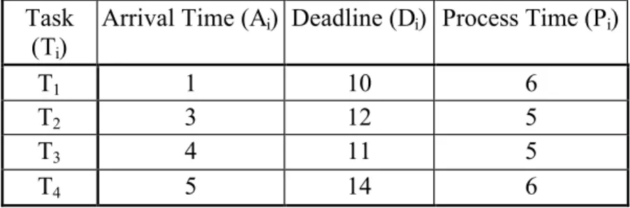
(11) 3.. If an element, Favail(C) ≥ 0 , exists in the reservation array, the PS schedule task T by using the rate code C. Task T is scheduled from the latest deadline backwards to the current time. Otherwise, the LC estimates power consumption Ptot of the base station according to the required bit rate. If the power, Ptot , is below the threshold, txadmit , then the PS assigns a new rate code C’ for the task T.. 4.. When all real-time tasks complete, the PS schedules non real-time tasks according to the elements of reservation array. If Favail(C) ≥ 0 exists, the PS schedules non real-time task T’ by using the rate code C. The radio resource can be assigned to task T’ that is based on the value of reservation elements. Otherwise, the LC estimates power consumption Ptot of the base station according to the required bit rate. If the power, Ptot, is below the threshold, txadmit , then the PS assigns a new rate code for the task T’.. Figure 4 illustrates a feasible, precise scheduling constructed using the reverse scheduling approach. In this example, we have four real-time tasks. Table 3 lists the parameters of the tasks. Figure 4 (a) – (d) show the timing diagrams of the tasks scheduling at time t = 1 to 5. In Fig. 4(a), task T1 arrives at time t=1. From reverse scheduling point of view, we schedule T1 in the interval (4, 9) using rate code C1. In Fig. 4(b), task T2 arrives at time t=3. We consider scheduling T2 using the same code C1. The reservation element of C1 is Favail(C1) = (D2 – t) – [(P2 – E2) + (P1 – E1)] = (12 – 3) – [6 + (7 – 2)] < 0 Since Favail(C1) < 0, T2 cannot complete transmission when the system uses only one channelization code. In this case, a new channelization code is considered for being assigned. The PS assigns a new channelization code C2 for task T2. The PS schedules T2 in the interval (7,12). Similarly, task T3 arrives at time t=4 (Fig. 4(c)) and the reservation element of C2 is,. Table 3 Task (Ti) T1 T2 T3 T4. Input parameters of real-time tasks.. Arrival Time (Ai) Deadline (Di) Process Time (Pi) 1 3 4 5. 10 12 11 14 11. 6 5 5 6.
(12) Rate C3 C2 C1. T1 Time. 1 2 3 4 5 6 7 8 9 10 11 12 13 14 15 16 17 A1. (Arrive/Deadline). D1. (a) t = 1 Rate C3 C2 C1. T2 T1. T1 Time. 1 2 3 4 5 6 7 8 9 10 11 12 13 14 15 16 17 A2. A1. D1. D2. (Arrive/Deadline). (b) t = 3. Rate C3 C2 C1. T3 T2. T2. T1. T1. 1 2 3 4 5 6 7 8 9 10 11 12 13 14 15 16 17 A1. A2 A3. D1. D2 D3. Time (Arrive/Deadline). (c) t = 4. Rate C3 C2 C1. T 3 NRT T2 NRT T1 T1. T3. T2 T4. 1 2 3 4 5 6 7 8 9 10 11 12 13 14 15 16 17 A1. A 2 A3 A 4. D1. D2 D3 D4. Time (Arrive/Deadline). (d) t = 5. Figure 4 An example illustrating the usage of RTIS algorithm.. Since Favail(C1) < 0, T2 cannot complete transmission when the system uses only one channelization code. In this case, a new channelization code is considered for being assigned. The PS assigns a new channelization code C2 for task T2. The PS schedules 12.
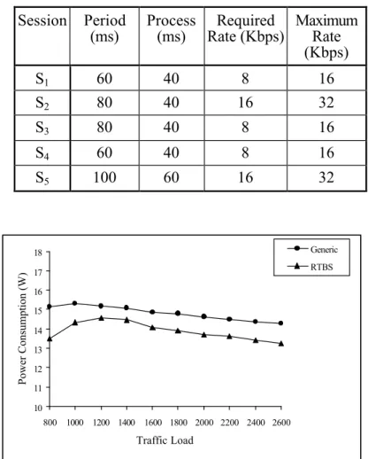
(13) T2 in the interval (7,12). Similarly, task T3 arrives at time t=4 (Fig. 4(c)) and the reservation element of C2 is, Favail(C2) = (D3 – t) – [(P3 – E3) + (P2 – E2)] = (11 – 4) – [5 + (6 – 1)] < 0 The PS assigns a new channelization code C3 for task T3 and schedules T3 in the interval (6,11). In Fig. 4(d), task T4 arrives at time t=5. Then, reservation element of C1 for task T4 is Favail(C1) = (D4 – t) – [(P4 – E4) + (P1 – E1)] = (14 – 5) – [6 + (7 – 4)] = 0 Since Favail(C1) = 0, that is, we can simultaneously apply code C1 to schedule task T1 and T4. Consequently, we can schedule T4 in the interval (8,14). When all real-time tasks are finished, there are still 3 units and 2 units of time reservation for C2 and C3, respectively. Consequently, the reservation times will be provided to schedule the non real-time tasks.. 4 Simulation results Experiments were performed to examine power consumption, session dropped rate and bandwidth utilization with traffic class to evaluate the performance of the proposed algorithms. The power consumption was measured when a base station allocated channelization codes for data session requests, based on the capacity analysis model of Eq. (1). The session dropped rate was calculated from the probability of rejected sessions. The experimental input parameters were as follows: The session requests were uniformly distributed. Session arrivals were Poisson distributed with mean arrival rate of A = 1 – 20 sessions/second. Session duration time was exponentially distributed with mean value of U = 100 seconds. The traffic load L is L = A × U . Each session involved contained several real-time tasks whose arrivals were periodic. The deadline of each task was equal to the period time. Table 4 shows the input parameters of possible period time, process time, guaranteed bit rate and max bit rate of task. We experimented 10000 session requests for each traffic load simulated. Figures 5 and 6 display the experimental results of RTBS algorithm versus Generic algorithm. The Generic algorithm defines that the management framework assigns a new rate code when a service request is arrive. Generic algorithm consumed the most power, and assigned a channelization code for each session arrival. RTBS, applying 13.
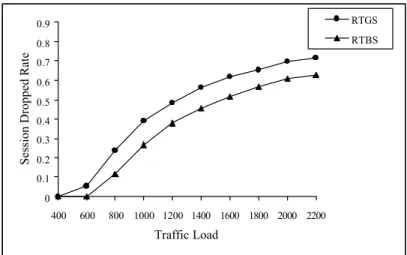
(14) the real-time EDF scheme that scheduled sessions’ tasks, is more cost-effective than generic algorithm. Figure 5 demonstrates the power consumption using Generic algorithm and RTBS as the traffic load increases from 800 to 2600. The respective power consumptions of Generic algorithm and RTBS are 15.14W and 13.49W for a traffic load of 800. The observed improvements in power consumption over that of Generic algorithm, varied to approximately 11% for RTBS. When the traffic load was 2600, the power consumption still improved to approximately 7.28 % for RTBS. Figure 6 plots session dropped rate against traffic load for Generic algorithm and RTBS. As shown in Fig. 6, the session dropped rate of Generic algorithm is 0.05, and that of RTBS is 0 for a traffic load of 600. For the heavy load simulation (traffic load=2200), the session dropped rates are 0.71 for Generic algorithm and 0.63 for RTBS.. Table 4 Selected input parameters for simulations. Session. Period (ms). Process Required Maximum (ms) Rate (Kbps) Rate (Kbps). S1 S2. 60 80. 40 40. 8 16. 16 32. S3. 80. 40. 8. 16. S4. 60. 40. 8. 16. S5. 100. 60. 16. 32. Generic. Power Consumption (W). 18. RTBS. 17 16 15 14 13 12 11 10 800. 1000 1200 1400 1600 1800 2000 2200 2400 2600. Traffic Load. Figure 5 Power consumption of algorithms versus traffic load.. 14.
(15) Session Dropped Rate. 0.9. RTGS. 0.8. RTBS. 0.7 0.6 0.5 0.4 0.3 0.2 0.1 0 400. 600. 800 1000 1200 1400 1600 1800 2000 2200. Traffic Load. Figure 6 Session dropped rate of algorithms versus traffic load.. Power Consumption (W). Figure 7 displays the power consumption of of RTIS versus Generic algorithm as the load increases from 100 to 280. The power consumption is 11.50W for Generic algorithm and 6.11W for RTIS at a traffic load of 100. When the traffic load is 280, the power consumption is still improved by 8.45 % for RTIS. Figure 8 depicts that the session dropped rates are 0.02 for Generic algorithm and 0 for RTIS at a traffic load of 100. In the heavy load simulation (traffic load=280), the session dropped rates of Generic algorithm and RTIS were 0.58 and 0.29, respectively.. 18 17 16 15 14 13 12 11 10 9 8 7 6. Generic RTIS. 100. 120. 140. 160. 180. 200. 220. 240. 260. 280. Traffic Load. Fig. 7 Power consumption of RTIS versus traffic load.. 15.
(16) Session Dropped Rate. 0.8. Generic. 0.7. RTIS. 0.6 0.5 0.4 0.3 0.2 0.1 0 100. 120. 140. 160. 180. 200. 220. 240. 260. 280. Traffic Load. Fig. 8 Session dropped rate of RTIS versus traffic load.. 5 Conclusions This work has proposed two real-time algorithms for packet scheduling. The proposed algorithms apply the functionalities of the management framework and the capacity analysis model to decide the threshold power for newly admitted real-time sessions. The real-time bandwidth scheduling (RTBS) makes the schedulable analysis that schedules the real-time data sessions to save power, using the EDF scheme. The real-time imprecise scheduling (RTIS), based on the imprecise computation, is constructed using the reverse scheduling approach. This scheme is greedy in that it schedule as much non real-time packets as possible after setting enough radio resource for all the arrived real-time packets. Experimental results verify that the proposed algorithms perform best in terms of power consumption and session dropped rate.. References [1]. S. Dixit, Y. Guo and Z. Antoniou, “Resource management and quality of service in third-generation wireless networks,” IEEE Comm. Mag., vol. 40, Feb. 2001, pp. 125-133.. [2]. 3GPP, IP Multimedia Subsystem (Release 5); TS 23.228, 2001.. [3]. G. AP Eriksson, B. Olin, K. Svanbro and D. Turina “The challenges of voice-over-IP-over-wireless,” Ericsson Review, No. 1, 2000, pp. 20-31. 16.
(17) [4]. Ö. Gürbüz and H. Owen, “Dynamic resource scheduling strategies for QoS in W-CDMA,” Proc. IEEE. GLOBECOM ‘99, vol. 1a, Dec. 1999, pp. 183-187.. [5]. L. Jorguseski, E. Fledderus, J. Farserotu and R. Prasad, “Radio resource allocation in third-generation mobile communication systems,” IEEE Comm. Mag., vol. 40, Feb. 2001, pp. 117-123.. [6]. S. K. Das, R. Jayaram, N. K. Kakani, and S. K. Sen, “A call admission and control scheme for quality-of-service (QoS) provisioning in next generation wireless networks,” Wireless Networks, June 2000, pp. 17-30.. [7]. A. Mittal and G. Manimaran, “Integrated dynamic scheduling of hard and QoS degradable real-time tasks in multiprocessors systems,” Fifth International Conference on Real-Time Computing Systems and Applications, Proceedings, 1998, pp. 127-136.. [8]. V. Millan-Lopez, W. Feng, and J. W.-S. Liu, “Using the imprecise-computation technique for congestion control on a real-time traffic switching element,” International Conference on Parallel and Distributed Systems, 1994, pp. 202-208.. [9]. 3GPP, UTRA High Speed Downlink Packet Access; Overall description (Release 5); TS 25.308, 2001.. [10] K. Hiltunen and R. D. Bernardi, “WCDMA downlink capacity estimation,” IEEE VTEC2000, 2000, pp. 992-996. [11] H. Holma and A. Toskala, WCDMA for UMTS. Nokia, Finland, Wiley, 2000. [12] W. K. Shih and J. W.-S. Liu, “Algorithms for scheduling imprecise computations with timing constraints to minimize maximum error,’ IEEE Trans. Comput., vol. 44, no. 3, Mar. 1995, pp. 466-471.. 17.
(18)
數據
+5

相關文件
Wang, Solving pseudomonotone variational inequalities and pseudocon- vex optimization problems using the projection neural network, IEEE Transactions on Neural Networks 17
We explicitly saw the dimensional reason for the occurrence of the magnetic catalysis on the basis of the scaling argument. However, the precise form of gap depends
Define instead the imaginary.. potential, magnetic field, lattice…) Dirac-BdG Hamiltonian:. with small, and matrix
Monopolies in synchronous distributed systems (Peleg 1998; Peleg
Akira Hirakawa, A History of Indian Buddhism: From Śākyamuni to Early Mahāyāna, translated by Paul Groner, Honolulu: University of Hawaii Press, 1990. Dhivan Jones, “The Five
Microphone and 600 ohm line conduits shall be mechanically and electrically connected to receptacle boxes and electrically grounded to the audio system ground point.. Lines in
* All rights reserved, Tei-Wei Kuo, National Taiwan University, 2005..
The remaining positions contain //the rest of the original array elements //the rest of the original array elements.
