通大學]
On: 28 April 2014, At: 03:34 Publisher: Taylor & Francis
Informa Ltd Registered in England and Wales Registered Number: 1072954 Registered office: Mortimer House, 37-41 Mortimer Street, London W1T 3JH, UK
International Journal of
Production Research
Publication details, including instructions for authors and subscription information: http://www.tandfonline.com/loi/tprs20
The construction of
production performance
prediction system
for semiconductor
manufacturing with
artificial neural networks
C.-L. HuangPublished online: 15 Nov 2010.
To cite this article: C.-L. Huang (1999) The construction of production
performance prediction system for semiconductor manufacturing with artificial neural networks, International Journal of Production Research, 37:6, 1387-1402, DOI: 10.1080/002075499191319
To link to this article: http://dx.doi.org/10.1080/002075499191319
PLEASE SCROLL DOWN FOR ARTICLE
Taylor & Francis makes every effort to ensure the accuracy of all the information (the “Content”) contained in the publications on our platform. However, Taylor & Francis, our agents, and our licensors make no representations or warranties whatsoever as to the accuracy, completeness, or suitability for any purpose of the Content. Any opinions and views expressed in this publication are the opinions and views of the authors, and are not the views of or endorsed by Taylor & Francis. The accuracy of the Content should not be relied upon and should be independently verified with primary sources of information. Taylor and Francis shall not be liable for any losses, actions, claims,
connection with, in relation to or arising out of the use of the Content. This article may be used for research, teaching, and private study purposes. Any substantial or systematic reproduction, redistribution, reselling, loan, sub-licensing, systematic supply, or distribution in any form to anyone is expressly forbidden. Terms & Conditions of access and use can be found at http://www.tandfonline.com/page/terms-and-conditions
The construction of production performance prediction system for
semiconductor manufacturing with arti® cial neural networks
C.-L. HUANG²
§
, Y.-H. HUANG² , T.-Y. CHANG³ , S.-H. CHANG§
, C.-H. CHUNG³ , D.-T. HUANG³ and R.-K. LI² *The major performance measurements for wafer fabrication system comprise WIP level, throughput and cycle time. These measurements are in¯ uenced by various factors, including machine breakdown, operator absence, poor dispatch-ing rules, emergency order and material shortage. Generally, production man-agers use the WIP level pro® le of each stage to identify an abnormal situation, and then make corrective actions. However, such a measurement is reactive, not proactive. Proactive actions must e ectively predict the future performance, ana-lyze the abnormal situation, and then generate corrective actions to prevent per-formance from degrading. This work systematically constructs arti® cial neural network models to predict production performances for a semiconductor manu-facturing factory. An application for a local DRAM wafer fabrication has demonstrated the accuracy of neural network models in predicting production performances.
1. Introduction
Three major performance measurements in a wafer fabrication consist of the WIP level, throughpu t (move volume
)
and cycle time. The relationship s among these performance measurements and the disturbance factors (e.g. machine break-down, material shortage and emergency order)
are quite complicated. For instance, machine breakdown may increase the WIP level, prolong the cycle time, and thereby in¯ uence the throughput of the downstream stages even further. A circumstance in which disturbance events occur daily poses di culty for the production manager to maintain system performance. Therefore, the undesirable e ects must be known in advance so that the proper corrective actions can be taken to prevent degrading performance. In practice, production managers use the WIP level pro® le of each operation stage to identify an abnormal situation and make necessary correcting actions. Such a measurement is reactive, not proactive. A proactive way must predict the future performance, identify and analyze an abnormal situation, and then gen-erate necessary corrective actions to prevent abnormal performance decreasing.Several models, including simulation, queueing, spreadsheet, regression and neural networks, can be employed to predict production performance. Of these,
0020± 7543/99 $12.00Ñ 1999 Taylor & Francis Ltd.
Final draft received April 1998.
² Department of Industrial Engineering and Management, National Chiao Tung University, 1001 Ta Hsueh Road, Hsinchu, Taiwan 30050, Republic of China.
³ Production Control Department, Mosel Vitelic Inc., Hsinchu, Taiwan, Republic of China.
§Department of Industrial Engineering and Management, Minghsin Institute of Technology, Hsinchu, Taiwan, Republic of China.
* To whom correspondence should be addressed.
simulation, regression and neural networks are the most widely used. In order to build a simulation model to predict and control the performance of a system subject to disturbances, the characteristics of these disturbances must ® rst be estimated and used as input variables. Then by introducing changes in these characteristics their e ect on the system performances (output variable
)
can be methodically evaluated. However, considering all the system disturbances in one simulation model is ex-tremely di cult. Moreover, detailed simulations require an enormous amount of time and money to write and maintain, especially in the semiconductor manufactur-ing environment; in addition, several hours are necessary to run them even on a powerful computer (Connors et al. 1996)
. Besides this, the accuracy in predicting wafer fabricatio n performance with simulation model still remains questionable due to its dynamic nature and complexity.Multiple regression is a general statistical technique used to analyze the relation-ship between a single dependent (predicted
)
variable and several independent ones (predictors)
. Multiple linear regression produces a linear approximation to ® t the data. Variable transformation allows, to some extent, the linear regression methods to handle nonlinear cases. However, such a transformation may make it di cult to interpret the results. We could always ® nd a polynomial of a higher degree that would yield a perfect ® t to a speci® ed data set. Thus, this results in over® tting and an inability of the regression model to generalize (Shyur et al. 1996)
.Neural networks are becoming more and more well known, and have been successfully implemented in manufacturing (Udo 1992, Zhang and Huang 1995
)
. For instance, Philipoom et al. (1994)
using neural network models, forecast the order due-date in a ¯ ow shop manufacturing system. The neural network model yielded better forecasting results than conventiona l due-date assignment approaches (Philipoom et al. 1994)
.Using historical data as the input variables, the regression model and neural network model can represent the properties and variations of a system. When a system is stable, acceptable forecasting accuracy using the two models is expected. However, ® nding a nonlinear regression model that can correspond to the historical data and represent the system’ s status is di cult. Many independen t variables must be considered in our case. Furthermore, some of the data do not ® t the basic assumptions of regression models. Thus, additiona l data transformations are necess-ary to generate our regression model. Alternatively, creating neural network models does not have the above conditions. Moreover, in practice, neural network models can yield better results than regression models (Philipoom et al. 1994, Shyur et al. 1996
)
. Using the neural network models to predict wafer fabrication’ s production performance has the following merits.(1
)
Neural networks can obtain a probable result even if the input data are incomplete or noisy.(2
)
A well-trained neural network model can provide a real time forecasting result.(3
)
Creating a neural network model does not necessitate understanding the complex relationship among input variables.Back-propagation neural networks (BPN
)
are widely used, and they produce good results in prediction and pattern recognition. Therefore, this work attempts to con-struct BPN prediction models. According to the ® eld managers’ experiences, WIP level and wafer move in previous time periods and upstream operation stages areselected as the input variables in our BPN model. A systematic construction pro-cedure is presented in the third section.
2. Neural network models
Neural networks are computing systems that incorporate a simpli® ed model of the human neuron, organized into networks similar to those found in the human brain. Arti® cial neural networks are computer simulations of biologica l neurons. Neural networks are composed of processing elements (nodes
)
and connections. Each processing element has an output signal that fans out along the connections to the other processing elements. Each connection is assigned a relative weight. A node’s output depends on the threshold speci® ed and the transfer function. The two types of learning are supervised and unsupervise d. For supervised learning, a set of training input vectors with a corresponding set of target vectors is trained to adjust the weights in a neural network. For unsupervised learning, a set of input vectors is proposed; however, no target vectors are speci® ed. Our approach towards the per-formance prediction problem is based on supervised neural networks. Supervised learning neural network models include back-propaga tion, counter-propagation net-work and learning vector quantization , of which, the back-propaga tion model is most extensively used and is therefore selected here.A back-propag ation neural network (BPN
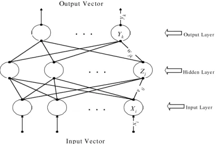
)
can be layered into many levels, with or without hidden layers exhibited between an input and an output layer. Figure 1 illustrates a network of neurons that are organized into a three layer hierarchy. Back-propagation learning employs a gradient-descent algorithm (Rumelhart and McClelland 1989)
. Through a supervised learning rule, the collected training data set comprises an input and an actual target output. The gradient-des cent learning algor-ithm enables a network to enhance the performance by self-learning. Two phases are availabl e for computation: forward and backward. In the forward phase of back-propagatio n learning, the input data pattern is directly passed into the hidden layer. Each element of the hidden layer calculates an activation value by summing up theZj Xi Yk w jk v ij
. . .
. . .
. . .
yk Output Ve ctor Input Vector xi Output Layer Hidden Layer Input LayerFigure 1. An example of three-layer backpropagation neural network.
weighted inputs and then transforms the weighted input into an activity level by using a transfer function (the sigmoid function is broadly used
)
. The resulting activ-ity is allowed to spread through the network to the output layer. If a di erence arises, i.e. an error term, the gradient-des cent algorithm is used to adjust the con-nected weights, in the backward phase. This learning process is repeated until the error between the actual and desired output (target)
converges to a prede® ned threshold. A trained neural network is expected to predict the output when a new input pattern is provide to it.In the backward phase, the network output ykis compared with the target value
tk to determine the associated error for that pattern with that unit. Based on this
error, the factord k is computed. d k is used to distribute the error at output unit Yk
back to all units in the previous layer (the hidden units that are connected to Yk
)
. It isalso used to update the weights between the output and the hidden layer. In a similar manner, the factord j is computed for each hidden unit Zj.d j is used to update the
weights between the hidden layer and the input layer.
After all the d factors have been determined, the weights for all layers are adjusted simultaneously. The adjustment to the weight Wjk (from hidden unit Zj
to output unit Yk
)
is based on the factord k , the activation zjof the hidden unit Zj,and the learning rate
h
. The adjustment to the weights vij (from input unit Xi tohidden unit Zj
)
is based on the factord j, the activatio n xiof the input unit, and thelearning rate
h
. The equation utilized to adjust the weights for the output layer k is D wjkh
d kzj,
where
D Wkj is the change to be made in the weight from the jth to kth unit,
h
is the learning rate,d k is the error signal for unit k,
zj is the jth element of the output pattern.
The back-propaga tion rule for changing weights for the hidden layer j is D vij
h
d jxi,
where
D vij is the change to be made in the weight from the ith to jth unit,
h
is the learning rate,d j is the error signal for unit j,
xi is the ith element of the input pattern.
3. BPN prediction model construction
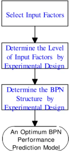
As ® gure 2 shows, constructing a BPN prediction model involves three steps: (a
)
performing correlation analysis to obtain proper input variables, (b
)
applying experi-mental design method to determine a good level combination of input variables, and (c)
applying an experimental design method to determine the optimum BPN struc-ture.3.1. Input factors selection
Creating a BPN model initially involve s determining the input variables. According to our observation in wafer fabrication, the following factors heavily in¯ uence the future performance of each operation stage.
(1
)
WIP levels of the current and previous two or three operation stages. (2)
Move volume of current and previous two or three operation stages. (3)
Disruptive factors such as machine breakdown, preventive maintenance,operator absence, and poor dispatching priorities.
The results presented here demonstrate that the ® rst two factors, WIP levels and move volume, are signi® cantly explanatory variables for the third one. Therefore, we select the ® rst two factors as our input variables.
The fact that the performances of previous days and the future performances of an operation stage correlate with each other necessitates that two further concepts, operation stage window and operation time window must be de® ned to construct a BPN prediction model.
Operation stage window: the total number of operation stages involved in con-structing the BPN prediction model, which include the current operation stage and previous operation stages. For instance, if the information retrieved for the BPN model includes only the current operation stage and the previous two operation stages, then the operation stage window = 3.
Operation time window: the size of time lagged to capture historical information from previous days. For instance, the information is captured from the current day and the previous two days to predict the performance of the current day. Then the operation time window = 3.
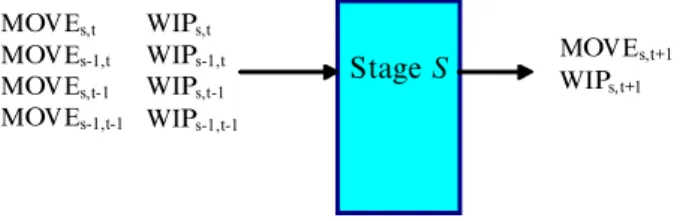
Figure 3 displays a BPN prediction model which is generated to predict the performance of stage S on date t+ 1 (MOVEs,t+ 1 and WIPs,t+ 1
)
, where t denotesthe observed day, and the input factors’ operation stage window = 2 and operation time window = 2.
Based on the data obtained so far, a correlation analysis has been performed to help determine the input variables. Table 1 depicts the correlation coe cients of the predicted performance and historical information from di erent input combination s
Select Input Factors
Determine the Level of Input Factors by Experimental Design Determine the BPN Structure by Experimental Design An Optimum BPN Performance Prediction Model
Figure 2. The BPN model construction procedure.
(operation stage windows and operation time windows
)
. The correlation coe cients shown in bold type are extremely high, indicating that the input variable s are accep-table. The p-values of this correlation analysis (H0:q = 0, H1:q 0)
are alsoex-amined, as listed in table 2. The p-values indicate that the predicted variables are not independent of the input variable s (p-value% 0.0001
)
. The three-day historical WIP levels and move volumes in operation stage s 1 do not correlate well with the predicted move volumes (p-value>
0.05)
, but they still correlate with the WIP level on date t+ 1; therefore, those input variables cannot be excluded. The same scenario arises for the three-day historical WIP levels, and move volumes in opera-tion stage s 2 do not correlate well with the WIP levels on date t 1.3.2. Determination of the operation time window and operation stage window The correlation analysis in section 3.1 allows us to con® rm the appropriaten ess of the input variables chosen by previous experience. However, not all the input vari-ables are expected to input to our model. In this study, the experimental design approach is employed to derive a better combination of operation stage window and operation time window so that the prediction error and model complexity can be reduced. By adopting previous experience, a 3 3 factorial design is generated. The operation stage window and operation time window are determined as the experi-mental factors (or treatments
)
. Each factor is classi® ed into three levels (table 3)
. Cumulatively, nine di erent BPN models are created.The data set used to perform the experiment, consisting of 180 records for six months of daily data, was collected from the Mosel Vitelic Inc., which is a famous DRAM wafer fabricator in Taiwan. These data include the normal and abnormal occurrences. All the examined stages are located in the following manu-facturing modules: photo, etching, thin ® lm and di usion. We delete 50 records whose data are not complete. To provide a mean for checking the BPN prediction against existing data, the remaining 130 records of available data are sub-divided into two sets. The ® rst set, called training data, is used to construct the prediction model. 106 records of training data are available . To prevent over-training , the second set, called testing data (24 records
)
, is used to assess the prediction model’s performance during the training process. This training process is repeated until the testing error, error between the actual and desired output from the testing data, converges to a prede® ned threshold value. The mean error percentage (MEP)
and coe cient of variance (CV)
are calculated to assess the performance of created BPN prediction models. Stage S WIPs,t WIPs-1,t WIPs,t-1 WIPs-1,t-1 MOVEs,t MOVEs-1,t MOVEs,t-1 MOVEs-1,t-1 MOVEs,t+1 WIPs,t+1Figure 3. The BPN prediction model for stage S.
T hr ee -d ay hi st or ic al W IP le ve ls o f st ag e s, s 1 an d s 2 P re di ct ed pe rf or m -St ag e s S ta ge s 1 S ta ge s 2 an ce s o f st ag e s on d at e t 1 s
,
t s,
t 1 s,
t 2 s 1,
t s 1,
t 1 s 1,
t 2 s 2,
t s 2,
t 1 s 2,
t 2 W IPs, t+ 1 0 .0 0 0 1 0 .0 0 0 1 0 .0 0 0 1 0 .0 0 0 1 0 .0 0 0 1 0 .0 0 0 1 -0. 63 75 -0. 98 99 0. 80 84 M o ves, t+ 1 0 .0 0 0 1 0 .0 0 0 1 0 .0 0 0 1 0. 16 67 0. 10 94 0. 07 33 0 .0 0 0 1 0 .0 0 0 1 0 .0 0 0 1 T hr ee -d ay hi st or ic al W IP le ve ls o f st ag e s , s 1 an d s 2 P re di ct ed pe rf or m -St ag e s S ta ge s 1 S ta ge s 2 an ce s o f st ag e s on d at e t 1 s,
t s,
t 1 s,
t 2 s 1,
t s 1,
t 1 s 1,
t 2 s 2,
t s 2,
t 1 s 2,
t 2 W IPs, t+ 1 0 .0 0 0 1 0 .0 0 0 1 0 .0 0 0 1 0 .0 0 0 1 0 .0 0 0 1 0 .0 0 0 1 0. 87 42 0. 89 53 0. 99 87 M o ves, t+ 1 0 .0 0 0 1 0 .0 0 0 1 0 .0 0 0 1 0. 05 59 0. 17 81 0. 33 26 0 .0 0 0 1 0 .0 0 0 1 0 .0 0 0 1 T ab le 2. T he p-va lu es fo r co rr el at io n an al ys is . T hr ee -d ay hi st or ic al W IP le ve ls o f st ag e s, s 1 an d s 2 P re di ct ed pe rf or m -St ag e s S ta ge s 1 S ta ge s 2 an ce s o f st ag e s on d at e t 1 s,
t s,
t 1 s,
t 2 s 1,
t s 1,
t 1 s 1,
t 2 s 2,
t s 2,
t 1 s 2,
t 2 W IPs, t+ 1 0 .9 3 6 1 4 0 .8 3 9 1 6 0 .7 7 2 5 6 0 .2 3 2 0 1 0 .2 4 7 2 6 0 .2 4 6 6 6 -0. 01 8 96 -0. 00 0 51 0. 00 9 67 M o ves, t+ 1 0 .6 5 5 6 3 0 .6 2 6 5 1 0 .6 1 2 1 -0. 05 5 61 -0. 06 4 35 -0. 07 1 99 -0 .2 7 6 7 1 -0 .2 7 4 8 5 -0 .2 8 2 1 4 T h re e-da y hi st or ic al M ov e vo lu m es of st ag e s , s 1 an d s 2 P re di ct ed pe rf or m -St ag e s S ta ge s 1 S ta ge s 2 an ce s o f st ag e s on d at e t 1 s,
t s,
t 1 s,
t 2 s 1,
t s 1,
t 1 s 1,
t 2 s 2,
t s 2,
t 1 s 2,
t 2 W IPs, t+ 1 0 .9 3 6 1 4 0 .8 3 9 1 6 0 .7 7 2 5 6 0 .2 3 2 0 1 0 .2 4 7 2 6 0 .2 4 6 6 6 -0. 01 8 96 -0. 00 0 51 0. 00 9 67 M o ves, t+ 1 0 .6 5 5 6 3 0 .6 2 6 5 1 0 .6 1 2 1 -0. 05 5 61 -0. 06 4 35 -0. 07 1 99 -0 .2 7 6 7 1 -0 .2 7 4 8 5 -0 .2 8 2 1 4 T ab le 1. T h e co rr el at io n co e ci en ts be tw ee n th e in p u t va ri ab le s an d pr ed ic te d va ri ab le s.mean error percentage (MEP
)
Y Y^ Y n %
,
coefficient of variance (CV
)
MSE/
X,
MSE Y ^Y 2 n 1
,
whereY is the historical value,
^
Y is the predicted value, and n is the sample size.
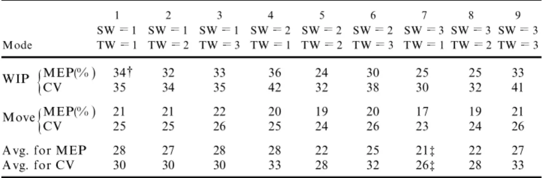
Owing to the limitations of time and cost, only ® ve di erent stages were ex-amined in this experiment. Although the results cannot be used to represent the entire production line, the same analysis procedure can be applied to analyse any operation stages in the entire production line. Table 4 summarizes the testing error and the performance judgment measures for all the nine WIP level and move volume prediction models. Hence, the average values of MEP used to identify the optimum model are calculated (table 5
)
, since the output layer includes the above two pre-dicted variables.The data are also examined by a two-way ANOVA analysis (table 6
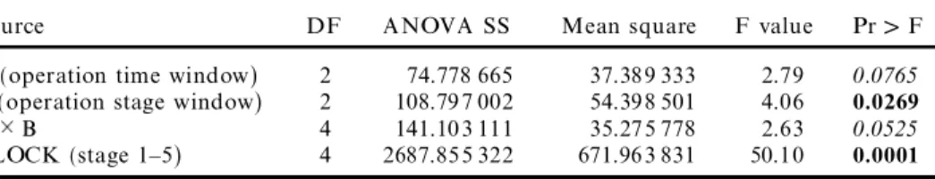
)
. Some of those results for a 5% signi® cance level can be summarized as follows.(1
)
The interactions between the operation time window and operation stage window are insigni® cant but close to the signi® cance level.(2
)
The factor e ects of the operation time window are insigni® cant. (3)
The factor e ects of the operation stage window are signi® cant. Based on the above experiment, we can conclude the following.Factors Levels
Operation stage window (SW) 1 Stage: (s) 2 Stages: (s,s 1) 3 Stages: (s, s 1,s 2)
Operation time window (TW) 1 day: (t) 2 days: (t, t + 1) 3 days: (t,t 1,t 2)
Table 3. Three levels for operation stage window and operation time window.
1 2 3 4 5 6 7 8 9 SW 1 SW 1 SW 1 SW 2 SW 2 SW 2 SW 3 SW 3 SW 3 Mode TW 1 TW 2 TW 3 TW 1 TW 2 TW 3 TW 1 TW 2 TW 3 WIP MEP(%
{
) 34² 32 33 36 24 30 25 25 33 CV 35 34 35 42 32 38 30 32 41 Move MEP(%{
) 21 21 22 20 19 20 17 19 21 CV 25 25 26 25 24 26 23 24 26Avg. for MEP 28 27 28 28 22 25 21³ 22 27
Avg. for CV 30 30 30 33 28 32 26³ 28 33
² A 5-stage average testing error (measured by MEP)for the WIP.
³ Minimum average predicted error for both WIP and Move.
Table 4. Prediction errors for WIP level and move volume.
(1
)
The optimum size of operation stage window (2 or 3)
can be derived from Duncan’ s multiple range test (Montgomery 1984)
, as shown in ® gure 4. (2)
Increasing the size of operation time window does not reduce the predictionerror, but increases the complexity of the prediction model.
(3
)
The optimum model exists when operation stage window = 3 and operation time window = 1.3.3. Determination of BPN model’s structure
A BPN model has an input layer, an output layer, and several hidden layers. Increasing the number of hidden layers increases the complexity of a BPN model. However, a guarantee does not exist that the model’s performance will be improved with an increasing number of hidden layers. Based on previous experience, only one
Operation time window
Errors (%) 1 day, (t) 2 days, t
,
t 1 3 days, t,
t 1,
t 2Operation 1 stage s 28 27 28
time 2 stages s
,
s 1 28 22 25window 3 stages s
,
s 1,
s 2 21² 22 27² Minimum average predicted error for WIP and Move.
Table 5. Mean error percentage (MEP)summary.
Source DF ANOVA SS Mean square F value Pr>F
A (operation time window) 2 74.778 665 37.389 333 2.79 0.0765 B (operation stage window) 2 108.797 002 54.398 501 4.06 0.0269
A B 4 141.103 111 35.275 778 2.63 0.0525
BLOCK (stage 1± 5) 4 2687.855 322 671.963 831 50.10 0.0001
Table 6. Two-way ANOVA analysis results for prediction errors (alpha 0.05, number of observations in data set 45).
Duncan Grouping
Mean (N=15) 23.574 25.061 27.354
Level of Operation stage
window 3 Stages 2 Stages 1 Stage
Figure 4. Duncan’s multiple range test for prediction errors (alpha 0.05).
Factors Levels
No. of hidden layers (HL) 1 layer 2 layers 3 layers
No. of hidden nodes for the hidden layer (HN) a b /4 a b /2 a b
Note a denotes the number of input nodes; b denotes the number of output nodes. Table 7. Three levels for the BPN structure.
or two hidden layers yield a better error convergence (Yei 1993
)
. The number of nodes in a hidden layer is another factor in¯ uencing the training process of creating a BPN model. Basically, more nodes in a hidden layer result in a smaller prediction error but a longer training time. Yei (1993)
also recommended the following prin-ciple to determine the number of hidden nodes for the hidden layer: HN (number of hidden nodes)
= (a + b)
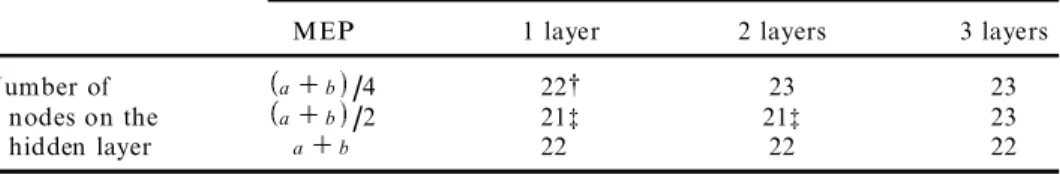
/2, where a denotes the number of input nodes and b denotes the number of output nodes.Sensitivity analysis is also performed to obtain a more re® ned structure of our BPN model. The previous BPN model with operation time window = 1 and opera-tion stage window = 3 are modi® ed by di erent numbers of hidden layers and nodes. Table 8 lists all the level’s combination s. From the average predicted error for WIP and Move shown in table 8, the following results are observed.
(1
)
The number of hidden nodes should be determined by Yei’s formula (HN = (a + b)
/2)
.(2
)
One or two hidden layers can yield a better prediction performance and therefore do not waste the training time.These predicted errors are examined by a two-way ANOVA analysis. Those results suggest that the di erences among predicted errors are insigni® cant. Therefore, advanced analysis does not have to be applied. The optimum case in table 8 was chosen to be the structure of our BPN prediction model.
3.4. An optimum BPN model
Only ® ve stages were examined in our experiment. However, these results can not be used to represent the actual circumstances of the entire wafer fabrication. According to the results of section 3.2 and 3.3, an optimum level’s combination
Number of hidden layers
MEP 1 layer 2 layers 3 layers
Number of a b /4 22² 23 23
nodes on the a b /2 21³ 21³ 23
hidden layer a b 22 22 22
² A 5-stage average testing error for the WIP and Move.
³ Minimum average error.
Table 8. Average predicted errors for WIP and Move.
Factors Levels
Operation stag window 3 stages SW 3
Operation time window 1 day TW 1
No. of hidden layers 1 or 2 layers HL 1 or 2)
No. of nodes on the (No. of inputs nodes No. of output nodes)/2 NH a b /2
hidden layers
Table 9. An optimum BPN structure.
was obtained by considering the minimum average prediction error for WIP and move volume. Table 9 lists the optimum level’s combinations.
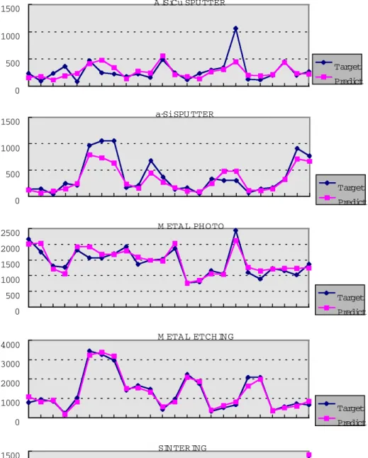
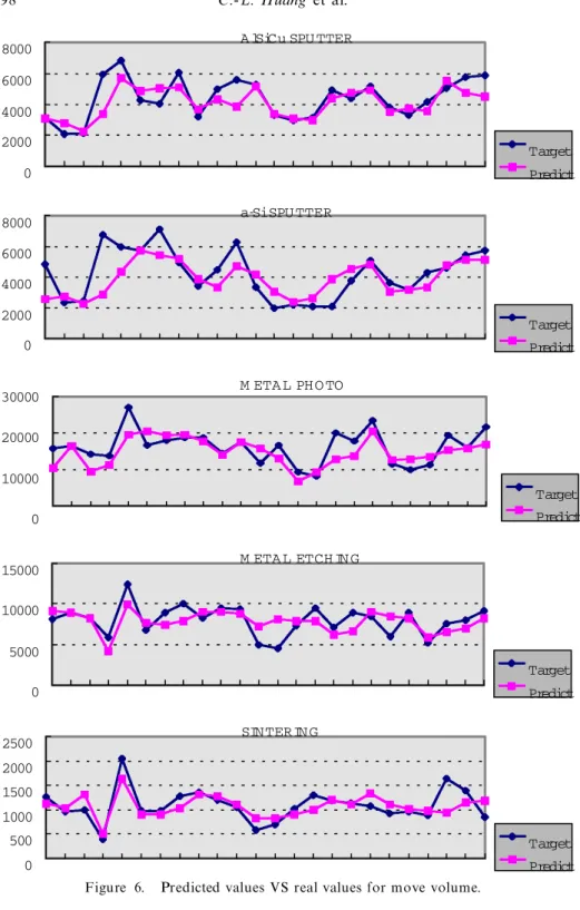
Figures 5 and 6 plot the predicted values and the real values: one for the WIP and the other for the move volume. As those ® gures reveal, using the optimum BPN
A lSiCu SPUTTER 0 500 1000 1500 Target Predict a-Si SPU TTER
0 500 1000 1500 Target Predict M ETAL PHOTO 0 500 1000 1500 2000 2500 Target Predict M ETAL ETCH ING
0 1000 2000 3000 4000 Target Predict SIN TERING 0 500 1000 1500 Target Predict
Figure 5. Predicted values VS real values for WIP level.
performance prediction model obtained herein has an average prediction error of only 21% .
Next the prediction errors were more closely examined. That examination con-® rmed a relationship between prediction error and the average variance of stage WIP
A lSiCu SPU TTER
0 2000 4000 6000 8000 Target Predict a-Si SPU TTER
0 2000 4000 6000 8000 Target Predict M ETAL PHO TO 0 10000 20000 30000 M ETAL ETCH IN G 0 5000 10000 15000 Target Predict SINTERIN G 0 500 1000 1500 2000 2500 Target Predict Target Predict
Figure 6. Predicted values VS real values for move volume.
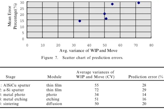
and move volume. In generally, an operation stage with a larger average variance has a large prediction error, as shown in table 10. Figure 7 depicts their relationships , as represented by the scatter chart. From this chart, a ® eld manager can realize that for the operation stage with a smaller average variance the predicted performance from the BPN prediction model is more reliable.
Moreover, a multiple regression model was compared with the neural network prediction model. The models can be expressed as
YMove
,
s,
t 1 b 0 b gijXgij e gij,
YWIP
,
s,
t 1 b 0 b gijXgij e gij,
where
Xgij are the input variables,
g is WIP or move, i s, s 1 or s 2, and
j t, t 1 or t 2.
By using the stepwise regression process, a prediction error of 26% was obtained. However, the prediction performance is not as high as the BPN model. For the cases presented here, the BPN prediction model is more appropriate than the regression model under the criteria of minimum prediction error.
4. M anagerial implications and implementation
The previous section explored how to select an optimum BPN prediction model to accurately predict wafer fabrication performance. Herein, we recommend using a two-stage (creating and running
)
implementation procedure to implement the BPN0 5 10 15 20 25 30 0 10 20 30 40 50 60 70 80
Avg. variance of WIP and Move
M ea n E rr or Pe rc en ta ge (% )
Figure 7. Scatter chart of prediction errors. Average variances of
Stage Module WIP and Move (CV) Prediction error (%)
1: AlSiCu sputter thin ® lm 55 28
2: a-Si sputter thin ® lm 72 29
3: metal photo photo 34 14
4: metal etching etching 51 16
5: sintering di usion 50 20
Table 10. Prediction errors and the variances of stage WIP and Move.
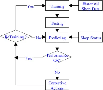
prediction model. Figure 8 illustrates the detailed process of these two stages. In the creating stage, the BPN model is trained by the new data obtained from the wafer fabrication. For this study, six months of information can adequately generate a good BPN prediction model.
In the running stage, the prediction results obtained from the BPN model are compared with the standard performance measures (standard WIP level and target move volume
)
. The di erence in this comparison (expressed as `low’ , `normal’, or `high’)
allows managers to quickly respond to any undesirable circumstances (table 11)
. The corrective actions are based on the interpretations of various combination s of low, normal and high levels of the predicted outputs. Hence, the way in which these levels are de® ned becomes very important. Logically, the reliability of this classi® cation into levels is bound to be highly dependent on the magnitude of the prediction error. Although an experienced manager can roughly determine the levels with his own experiences and adjust these levels accordingly, the quality aspect of the prediction control level should be further studied.De® ning a standard WIP level and a target move volume at any stage is quite complex. Although this issue is not discussed here, the manager’s experience and the historical data help us to obtain a rough standard: (1
)
standard WIP level, average WIP during the past one week; and (2)
target move, month output divided by the number of work days. For instance, if the month output is 36 000 wafers and there are 30 work days in a month, a rough target move for one stage may be 1200 wafers per stage daily. (36 000 wafers/30 work days = 1200 wafers/stage/day)
.Model retraining becomes necessary when a system is changed (e.g. new routing is added
)
. Otherwise, the current BPN model loses its ability to accurately predict the new system’s performance. The following criteria can be applied to determine the schedule for the model retraining: (1)
new routing is added, or (2)
cumulated pre-diction errors are outside the control limits after some time periods, e.g. two or three months. Training Testing Corrective Actions Performance OK?Predicting Shop Status
Yes
No
ReTraining ? No
Yes Shop DataHistorical
Figure 8. BPN prediction model’s implementation process.
P re d ic te d re su lt s W IP le ve l M ov e vo lu m e P o ss ib le re as o ns C or re ct iv e ac ti o n s M ac hi n e do w n o r p re ve nt iv e m ai nt en an ce (P M) R es ch ed ul e P M to k ee p n or m al m o ve s H ig h L o w M ac hi n e fo r en gi n ee ri n g u se (M ac h in e le nt ) A llo ca te m ac h in e p ro pe rl y to o bt ai n m o re m ov es M ac hi n e al lo ca te d fo r th e o th er st ag e S o lv e th e m ac hi n e o r o p er at io n p ro b le m s of d ow n st re am st ag e
{
Hig h W IP in d o w n st re am st ag e H ig h N o rm al H ig h m o ve s in up st re am st ag e B al an ce th e m o ve s in up st re am st ag e{
R ea llo ca te m ac h in e to ob ta in m o re m ov es an d to re du ce W IP L ow m o ve s in u ps tr ea m st ag e C h an ge th e lo t p ri o ri ty o f u p st re am st ag e to ob ta in m o re m o ve s M ac hi n e st ar va ti on d ue to lo w W IP fo r st ag e S L o w L o w M ac hi n e do w n o r P M in st ag e S or in u p st re am S o lv e th e m ac hi n e o r o p er at io n p ro b le m s of st ag e S o r up st re am st ag e st ag e E va lu at e th e im p ac ts o n do w ns tr ea m st ag e to av oi d d o w n st re am{
m ac h in e st ar va ti o n L ow m o ve s in u ps tr ea m S o lv e th e m ac hi n e o r o p er at io n p ro b le m s of th e u ps tr ea m st ag e L o w N o rm al N o n -b ot tl en ec k st ag e C h an ge th e lo t p ri o ri ty o f u p st re am st ag e to ob ta in m o re m o ve s fo r st ag e S{
O b ta in h ig he r W IP to av oi d st ar va ti o n N or m al L o w M ac hi n e al lo ca te d im p ro pe rl y E va lu at e th e im p ac ts o n do w ns tr ea m st ag e to av oi d d o w n st re am{
m ac h in e st ar va ti o n T ab le 11 . P o ss ib le re as o ns an d co rr ec ti ve ac ti o n s fo r lo w pe rf o rm an ce in st ag e S .Training is the most time-consuming process in creating a BPN model. However, a well-trained BPN model can satisfy the requirement of real time running. Many commercial neural network programs with a powerful learning ability and good user interfaces have been developed . Such tools can be easily adapted by managers. In addition, to conserve the model construction time, the BPN model can only be applied to the key stages (including the bottleneck stages
)
.5. Conclusion and future works
This work constructs a performance prediction model that is capable of provid-ing an advanced warnprovid-ing for the performance change of each operation stage in a DRAM wafer fabrication. The study of the BPN prediction model applied to a local wafer fabrication o ers promising results when using a three-layer back-propaga tion neural network, thereby allowing for a more accurate prediction of the WIP level and move volume in the next time period for each wafer fabrication operation stage. Experimental results demonstrate that the optimum model is available when the input nodes include all the previous day’s information (WIP level and move volume
)
for three continuous previous stages. Also, the prediction results con® rm that our model can provide a roughly 80% forecasting accuracy based on the exist-ing data. Based on the BPN model construction procedure presented in this study, the Mosel Vitelic Inc. is now planning to construct and implement the performance prediction system.Although the preliminary results are encouraging , additional study is necessary to improve the forecasting accuracy. In this study, the WIP level and move volume are the only two input variables. However, our models do not exhibit other factors that in¯ uence the production performance, such as machine breakdown and dis-patching rules. If more data can be obtained and new factors that can in¯ uence production performance can be included, more promising and meaningful models can be developed.
Ackno wledgment
The authors would like to thank the referees for their valuable comments and suggestions.
References
CONNORS, P., FEIGIN, G. E.andYAO, D. D.,1996, A queueing network model for
semicon-ductor manufacturing. IEEE Transactions On Semiconsemicon-ductor Manufacturing, 9, 412± 427.
MONTGOMERY, D. C.,1984, Design and Analysis of Experiments (New York: Wiley).
RUMELHART, D. E. and MCCLELLAND, J. L., 1989, Paralled Distributed Processing:
Explorations in the Microstructure of Cognition (Cambridge, MA: MIT Press).
PHILIPOOM, P. R., REES, L. P.andWIEGMANN, L.,1994, Using neural networks to determine
internally-set due date assignments for shop scheduling. Decision Sciences, 25, 825± 851.
SHYUR, H.-J., LUXHOJ, J. T. and WILLIAMS, T. P.,1996, Using neural networks to predict
component inspection requirements for aging aircraft. Computers and Industrial Engineering , 30, 257± 267.
UDO, G. J.,1992, Neural networks applications in manufacturing processes. Computers and
Industrial Engineering, 23, 97± 100.
YEI, I.-C.,1993, Neural Networks Applications and Practice (Taiwan: Zu-Lin Publishing).
ZHANG, H.-C.andHUANG, S.-H.,1995, Applications of neural networks in manufacturing: a
state-of-the-art survey. International Journal of Production Research, 33, 705± 728.