Adaptive self-quantization in wavelet-based fractal image compression

This article was downloaded by: [National Chiao Tung University 國立交通大學] On: 28 April 2014, At: 03:31

Publisher: Taylor & Francis

Informa Ltd Registered in England and Wales Registered Number: 1072954 Registered office: Mortimer House, 37-41 Mortimer Street, London W1T 3JH, UK

International Journal of Systems Science

Publication details, including instructions for authors and subscription information:

http://www.tandfonline.com/loi/tsys20

Adaptive self-quantization in wavelet-based

fractal image compression

Bing-Fei Wu , Yi-Qiang Hu & Hung-Hseng Hsu Published online: 26 Nov 2010.

To cite this article: Bing-Fei Wu , Yi-Qiang Hu & Hung-Hseng Hsu (1999) Adaptive self-quantization in wavelet-based fractal image compression, International Journal of Systems Science, 30:5, 541-549, DOI: 10.1080/002077299292281

To link to this article: http://dx.doi.org/10.1080/002077299292281

PLEASE SCROLL DOWN FOR ARTICLE

Taylor & Francis makes every effort to ensure the accuracy of all the information (the “Content”) contained in the publications on our platform. However, Taylor & Francis, our agents, and our licensors make no representations or warranties whatsoever as to the accuracy, completeness, or suitability for any purpose of the Content. Any opinions and views expressed in this publication are the opinions and views of the authors, and are not the views of or endorsed by Taylor & Francis. The accuracy of the Content should not be relied upon and should be independently verified with primary sources of information. Taylor and Francis shall not be liable for any losses, actions, claims, proceedings, demands, costs, expenses, damages, and other liabilities whatsoever or howsoever caused arising directly or indirectly in connection with, in relation to or arising out of the use of the Content.

This article may be used for research, teaching, and private study purposes. Any substantial or systematic reproduction, redistribution, reselling, loan, sub-licensing, systematic supply, or distribution in any form to anyone is expressly forbidden. Terms & Conditions of access and use can be found at http://www.tandfonline.com/page/terms-and-conditions

Adaptive self-quantization in wavelet-based fractal image

compression

Bing

-

Fei Wu² _{, Yi}

_-

_{Qiang Hu}² _{and Hung}

_-

_{Hseng Hsu}²

Finding a model to quantize the scale factors in wavelet-based fractal image com-pression is a complicated issue. To avoid error, it is helpful to model the distribution of the scale factors and quantize them before the computation process by iterated function systems. Traditionally, a ® xed model with uniform distribution was frequently adopted. This is not sophisticated enough, however, to quantize these scale factors from errors since, in general, the factors are not uniformly distributed. We propose an adaptive algorithm with self-quantization to overcome this drawback. Except for the functions of adaptation and self-quanti® cation, the approach has the optimal property that the fundamental objective is to reduce the quantization errors.

1. Introduction

In the application of image processing, discrete wavelet transforms (DWT) are employed to extract the coded image into several sub-images with di€ erent resolutions (Mallat 1989, Antonini et al. 1992, Strang and Nguyen 1996). The methods of image compression using DWT could provide high compression ratios (CR) and high image ® delity as well (Antonini et al. 1992, Vetterli and KovacÏevic 1995, Hsu et al. 1997). These subimages, except for the ones with lowest frequencies, which are similar to the original image in general, are called detailed images. Rinaldo and Calvagno (1995) further pointed out the redundancy of the wavelet-based images across scales from the perspective of fractals. Hence, it is said that an image performed after DWT has the intrinsic property of fractals and can be manipu-lated by fractal compression methods for further com-pressing this image e€ ectively. Moreover, the application of fractal coders to wavelet-based images over original images is highly recommended for the application’s ability to enhance the similarity among the detailed sub-images, but also to reduce the blocking e€ ect in most other block-based coding techniques since we extract the similarities in the frequency domain instead of the spatial domain.

A block coding method by means of the technique of Interactive Function Systems (IFS), introduced by Barnsley and Jacquin (1988) and Jacquin (1993), was widely used in fractal image compression. It has proven successful for compressing images at low bit rates. The main procedure of IFS is to ® nd and manip-ulate the domain block such that it can be the most matched one for a ® xed range block in some measure senses (Jacobs et al. 1992, Fisher 1994). Following that, we have to determine all the IFS parameters corre-sponding to the range blocks. The IFS maps can be iteratively applied to ® nd the ® xed point, which is an approximation to the image to be coded. To reduce the decoding time and error, this study presents a new prediction approach that di€ ers slightly from IFS. In the coding part of the predictor, the domain and range pools belong to di€ erent subbands with the same orien-tation and block size. The domain pool is constituted by the subimage with a lower frequency, thereby ensuring smaller values of scale factors since the image has the property of power `decayness’ (Antonini et al. 1992).

The IFS parameters include the positions of the domain blocks, eight isometries of the square achieved from the compositions of re¯ ections and 90ë _rotations,

scale factors and o€ set values. There is no doubt that the positions and isometries belong to integers and need not be quantized before coding them. However, generally, the scale factors and o€ set values should be ¯ oating numbers. We need to quantize them for coding. The main purpose of this paper will focus on the relationship of the quantization and IFS coding error. We try to ® nd 0020± 7721/99 $12.00Ñ 1999 Taylor & Francis Ltd.

Received 20 October 1997. Revised 28 May 1998. Accepted 29 May 1998.

² _{Department of Electrical and Control Engineering, National}

Chiao Tung University, Hsinchu, Taiwan; e-mail: [email protected]. edu.tw

a better way to avoid errors accumulating, under the situation that IFS coding is followed by quantization. A complete code including DWT, IFS and the entropy coding is addressed in our other work (Wu et al. 1997). The o€ set values here allow us to adjust the DC com-ponents of the range blocks (Antonini et al. 1992). More precisely, the o€ set values in IFS coding can be taken as the DC values corresponding to range blocks (Davis 1995). Naturally, we assume that the distribution of the o€ set values for all range blocks is similar to that of the encoded image. For the images performed after DWT, the distributions of detailed images can be mod-elled on generalized Gaussian distributions (Daubechies 1988). Hence, the distribution of the o€ set values was obtained and their quantization was found. Next, we will face a serious problem when quantizing these scale factors.

If we quantize the ¯ oating scale factors after IFS, the `second error’ will be introduced. That is the quantiza-tion error and the error induced by IFS would be com-pounded. A better way is to quantize these ¯ oating numbers before processing in IFS, provided that we know and model the histogram of these scale factors precisely. In fact, we have no idea how to model the histogram, other than the fact that the distribution of these scale factors was concentrated around zero and was decayed on both sides, and was observed from the experimental results. Therefore the simplest way is to approximate it with a uniform distribution (Jacquin 1993). This would result in a less optimal case for searching for IFS parameters. In this case we propose an Adaptive Self-Quantizer (ASQ) to overcome the above disadvantage in quantizing these scale factors. As we know, adaptivity will be a trend for lossless data compression in the future. It will do well in the case that the statistics of the input source are either unknown a priori or varying over time. Some recent work of adaptive quantization (Steinberg and Gutman 1993, Chan and Vetterli 1995) was designed with existing codebooks, which require background informa-tion. The objective of altering the support region of a uniform scalar quantization is also demonstrated in Jayant (1973), Crisafulli and Bitmead (1993); however, the modelling source is not adjustable. ASQ is initiated as a uniform model intuitively and is permitted to update the model adaptively according to the input values. Based on the adaptive model and inputs, the quantized outputs can also be self-adjusted. This means that no more bits are necessary to specify the codebook. After that, we acquire an e€ ective model and reduce the error in quantization of the scale factors. The concept of optimality is included in this algorithm to reduce quantization error. There are two approaches to reconstruct the coding data, the forward and back-ward methods, which depend on the necessary encoded

bits and the quality of the reconstructed image. Moreover, we apply the concept of the source modelling from Ortega and Vetterli (1997), which estimates the probability density function (p.d.f.) at the mid-point of the intervals by taking a matrix inversion through Gaussian substitution methods. However, we have esti-mated the p.d.f. at the values of decision levels by a kind of curve ® tting technology, Least Squared Error (LSE) method. Next, we also depict the distribution by linear interpolation. In addition, the approach can be consid-ered as one kind of adaptive ® lters (Widrow and Stearns 1985). We can ® nd the geometric ratio of the algorithm from the viewpoint of adaptive signal processing and consider the in¯ uence of the ratio to the adaptation capability and reconstruction ® delity.

The organization of this paper is as follows: the prob-lem of quantizing scale factors in fractal image com-pression is formulated in the next section. In section 3, we will introduce the algorithm of the adaptive self-quantizer, which is designed by three key points. The reconstruction procedures are also illustrated. After that, we will address some intrinsic properties about the algorithm. The experimental results, as listed in sec-tion 4, reveal that the adaptive self-quantizer is superior to the uniform model that was usually adopted before. As a result, a brief conclusion is made in the ® nal sec-tion.

2. Problem formulations and notations

We will put more emphasis on the quantization of the scale factors, for it plays an important role in fractal block coding. In order to quantize the scale factors e€ ec-tively, more precisely, and to reduce the composite errorsÐ which are produced by fractal coding errors and quantization errorsÐ we shall introduce ASQ before applying the IFS coding.

2.1. Problem formulations

Let us formulate the quantization problem ® rst. Consider a d-bit scalar quantizer, then there are 2d output levels corresponding to 2d input intervals. The I/O relationship of a 2-bit scalar quantizer is shown in ® gure 1.

542 Bing-Fei Wu et al.

Figure 1. A 2-bit scalar quantizer.

2.2. Notation

For convenience in depicting the ASQ algorithm, we should de® ne the notations of the d-bit scalar quantizer.

d: bits of the quantizer; nf: the number of scale factors;

S

(

n

)

: the nth scaling factor, for n2 N

7

f 1,2,. . .,n_fg ;

~

S

(

n

)

: the estimated input;

d j(n): decision levels at stage n of the quantizer, j2 Q

­

f 2dg , where Q

7

f 1,. . .,2d_g ;

y(in)

[

d (i­n)1,d i(n)

]

, for i2 Q

­

f 1,2dg ,

(­

1 ,d 1(n)

]

, for i

=

1,

[

d (₂nd)_­1,1

)

, for i

=

2d,

which are called the ith interval of the quanti-zer;

Xi(n): the number of elements in y(in),i2 Q. It is also called the ith counter. Moreover, Xi(n)/n can be considered as the probability in y(i ;n)

m(in): reconstructed levels at stage n of the quantizer, i2 Q.

3. Adaptive Self-Quantizers

In fractal block coding, the uniform models were usually adopted to quantize the scale factors since we cannot obtain their distribution in advance. Unfortunately, in general, the scale factors would not be uniformly distributed. Hence, we have the idea of designing an adaptive quantizer that can self-adjust the model to an appropriate one. The key points of ASQ are in the following statements.

(1) The distribution of these scale factors without quan-tization concentrates around zero and decays on both sides in general. That is, the distribution is a model with smoothly decaying tails (Ortega and Vetterli 1997). When applying fractal coding to a detailed subimage, the concentrating histogram phenomenon can be seen in ® gure 2.

(2) The ASQ satis® es the optimal solution in a scalar quantizer (Max 1960, Hang and Woods 1995, Wu and Hsu 1996). That is,

1. the reconstruction level is the centroid of the interval, and

2. the decision level is the average of neighbouring reconstruction levels.

(3) The more concentrated the histogram, the smaller the interval.

Before illustrating the ASQ algorithm, we need to make an initialization.

d (_j0): the values to decide, such that we can uni-formly split into 2d intervals for some rea-sonable range R, j2 Q

­

f 2d};

d (₀0),d (₂0d): the values used to de® ne the dynamic range R of ASQ;

m(i0): the centroids are initially chosen to be the mid-point of the ith interval;

Xi(0): the counters are all set to unity; where j2 Q

­

2d and i2 Q..

After initializing the algorithm, a uniform model fol-lows. In other words, we suppose that ASQ starts run-ning from a uniform model.

3.1. The ASQ Algorithm

We depict the ASQ algorithm as follows (see equa-tions (1)± (9) at top of next page).

The ASQ algorithm will stop when the input sequence S

(

n

)

is terminated (n

₌

nf). The coding data include the integer terms: S^

(

n

_{) =}

i, for n

₌

1,2,. . .,nf, and, if necessary, the ¯ oating terms: m(nf)

j , for j2 Q.

Remarks: The choice of a and b (a<b) in the ASQ

algorithm depends on the ® rst key point shown before such that the estimated inputS~

(

n

)

can be located at the position closer to the origin. For example, we set a

₌

1 and b

₌

2. It is observed that the choice of a and b will a€ ect the quantization error. Detailed discussion for di€ erent values of a/b will be illustrated in the next section. We will estimate the shape of the source distri-bution linearly by the parameters a and b.

3.2. Reconstruction of ASQ algorithms

There are two approaches to reconstruct the coding data, which depend on the necessary encoded bits and

Figure 2. The histogram of scale factors without quantization in Dh2: the horizontal oriented subimage with resolution14

per-formed after DWT.

the quality of the reconstructed image. One approach is called the forward method. The meaning of `forward’ is that the reconstructed procedure follows an ASQ algor-ithm directly. That is, we repeat the ASQ algoralgor-ithm from n

₌

1 to nf by means of S^

₍

n

₎

, for n

₌

1,2,. . .,n_f and the default initialized model (R is known). Another approach is called the backward method. `Backward’ represents that the fact we can rebuild the quantized values from n

₌

nf to 1 by the use of the coding data

^

S

(

n

)

and m(nf)

j , for n

=

1,2,. . .,nf and j2 Q.

The di€ erences between these two methods are as follows.

•

The forward method only needs to store the integer term S^

(

n

)

of the coding data. No more bits are required to quantize the scale factors. However, the initial model must be ® xed and considered as a default model in advance.

•

The backward method must save all coding data including integer and ¯ oating terms. We can reduce the quantization error at the cost of having to assign more bits to code these ¯ oating terms. However, it is unnecessary to be concerned with the initial model. But we can try to look for better solutions for di€ er-ent initial models, or di€ erer-ent values of R.

544 Bing-Fei Wu et al. for S

(

n

)

2 y(in­1), ~ S

(

n

_{) =}

ad _i(_­n­₁1) +bd (in­1) a+b

=

am(_i­n­₁1)+

(

a+b

₎

m(in­1)+bm(i+n­11) 2

(

a+b

)

,i2 Q1

7

f 1,. . .,2d­1g bd i(­n­11) +ad (in­1) a+b

=

bm(i­n­11)+

(

a+b

)

m(in­1)+a(i+n­11) 2

(

a+b

)

,i2 Q2

7

f 2d­1+1,. . .,2dg ,

(

1

)

Xj(n)

=

Xi(n­1) +1, for j

=

i, Xj(n­1), for j6

=

i,

(

2

)

m(in)

=

m (n­1) i Xi(n­1)+S~

(

n

)

Xi(n) ,

(

3

)

Case I. i2 Q1 mj(n)

=

mj(n­1), for j>i,

(

4

)

mj(n)

=

m(jn­1)+mi(n)

­

m(in­1), for j<i,

(

5

)

d (_in)

₌

m (n) i +m(i+n)1 2 d j(n)

=

d j(n­1), for j>i, d (jn)

=

d (jn­1)+m(in)

­

m(in­1)

=

m(_jn)+m(_j+n)₁ 2 , for j<i, d _k(n)

₌

m (n) k +m( n) k+1 2 ,for k2 Q1.

(

6

)

Case II. i2 Q2 mj(n)

=

mj(n­1), for j<i,

(

7

)

mj(n)

=

m(jn­1)+mi(n)

­

m(in­1), for j>i,

(

8

)

d (in)

=

m(in)+m(i+n)1 2 d j(n)

=

d j(n­1), for j<i

­

1, d (jn)

=

d (jn­1)+m(in)

­

m(in­1)

=

m(jn)+m(j+n)1 2 , j,. . . >i

­

1, d k(n)

=

m(kn) +m(k+n)1 2 ,for k2 Q2.

(

9

)

3.2.1. The forward method. According to the default initial model and S^

(

n

)

, the ASQ algorithm repeats it-self. For each stage n, we pick out the reconstruction level m(in), where i

=

^

S

(

n

)

. During this time we can ob-tain the reconstructed values of scale factors for n

₌

1,2,. . .,nf.

3.2.2. The backward method. In order to run the back-ward method, we need to have the coding data which include the integer terms: S^

(

n

_{) =}

i, for n

₌

1,2,. . .,nf, and the ¯ oating terms: m(nf)

j , for j2 Q. The course of the backward method is listed as follows:

(1) constitute X(nf) i , i2 Q, by means of ^ S

(

n

)

, for n

₌

1,2,. . .,n_f; (2) rebuild Xi(n­1): Xi(n­1)

=

Xi(n)

­

1, i

=

^ S

(

n

)

, Xi(n), otherwise; (3) reconstruct m(in­1): (i) i2 Q1: mj(n­1)

=

mj(n), for j>i, m(in­1)

=

[

2

(

a+b

)

Xi(n)+a

]

mi(n)

­

am(i­n)1

­

bm(i+n)1 2

₍

a+b

)

Xi(n­1) +2a+b , mj(n­1)

=

mj(n)

­

[

mi(n)

­

m(in­1)

]

, for j<i; (ii) i2 Q2: mj(n­1)

=

mj(n), for j<i, m(in­1)

=

[

2

(

a+b

)

Xi(n)+a

]

mi(n)

­

bm(i­n)1

­

am(i+n)1 2

(

a+b

)

Xi(n­1) +2a+b , mj(n­1)

=

mj(n)

­

[

mi(n)

­

m(in­1)

]

, for j>i. For each stage n, we choose the reconstruction level m(in), where i

=

^

S

(

n

)

. Therefore we can obtain the recon-structed values of scale factors for n

₌

1,2,. . .,n_f.

3.3. Another version of ASQ algorithms

In the previous subsection, we estimated the decaying property of the distribution from the choices a and b. That is, we must decide the values of a and b before running the ASQ algorithm. Therefore, the perform-ances of ASQ algorithms depend heavily on the selection of a and b. But there seems to be a lack of robustness. In order to increase the robustness, the idea of estimating the decaying distribution by ® xed values of a and b has to be replaced by another di€ erent concept: that is, to estimate the p.d.f., which is taken as the values at deci-sion levels by the LSE method. The concept of Ortega and Vetterli (1997) estimates the p.d.f. at the mid-points of intervals and therefore obtains the solution by taking a matrix inversion through the Gaussian substitution methods. After determining the estimated p.d.f.,_^ f

(

d j(n)

)

, j2 Q

­

f 2dg , we can rebuild the source distri-bution more successfully by interpolating the estimated p.d.f. linearly. So, the value ofS~

(

n

)

in (1) is substituted by the centroid of the ith interval in stage n for more robustness.

Let us describe this course in detail. In de® ning the accumulated probability at the ith interval in stage n as P(in) and P(in)

=

X (n) i n+ k2 QXk(0) ,

=

di di­1 ^ f

(

x

)

dx,

=

1₂

(

d i

­

d i­1

)

f ^ f

(

d i

)

+ ^ f

(

d i­1

)

g ,

(

10

)

we assume that the p.d.f. at boundary points are set to zeros, i.e., f^

(

d (0n)

) =

^

f

(

d ₂(nd)

) =

0. Hence, (10), for i2 Q,

can be represented as a matrix form (see at bottom of page).

We abbreviate the matrix equation as F

₌

2P, where T

₇

_[

_u

₍

₁

₎

_u

₍

₂

₎

_u

₍

₂d

₎

_]

_{, u}

_{( )}

_{is a}

₍

₂d

_­

₁

₎

₁ column vector, F

7

[

f^

(

d ₁(n)

)

f^

(

d ₂(n)

)

f^

(

d ₂(nd)_­1

)

]

T and Y

7

[

P(1n) P2(n) P(2nd)

]

T. This is inconsistent, generally,

since there are 2d

_­

1 unknown parameters and 2d

equa-1 2 d ₁(n)

­

d ₀(n) 0 0 0 0 0 0 d 2(n)

­

d (1n) d 2(n)

­

d (1n) 0 0 0 0 0 0 d ₃(n)

­

d (₂n) d ₃(n)

­

d ₂(n) 0 0 0 0 .. . . . . .. . 0 0 0 0 0 d ₂(nd)_­1

­

d ( n) 2d_­2 d ( n) 2d_­1

­

d ( n) 2d_­2 0 0 0 0 0 0 d ₂(nd)

­

d ( n) 2d_­1 ^ f

(

d (₁n)

)

^ f

(

d (2n)

)

^ f

(

d (₃n)

)

.. . ^ f

(

d (₂nd)_­2

)

^ f

(

d (₂nd)_­1

)

=

P(1n) P(2n) P(3n) .. . P(₂nd)_­1 P(₂nd) .

tions in this matrix equality. Therefore, we will take the LSE solution

FLSE

= (

T

)

­1 T

(

2P

)

,

(

11

)

where FLSE

7

[

fLSE

(

d 1

)

fLSE

(

d 2d_­1

)

]

T. It is a

time-con-suming task to obtain the oƒ ine solution in (11). The least squared solution can be acquired by a recursive form as follows (Goodwin and Sin 1984):

PF

(

k

) =

PF

(

k

­

1

) ­

PF

(

k

­

1

)

u

(

k

)

u T

₍

_k

₎

_P F

(

k

­

1

)

1+u T

(

k

)

PF

(

k

­

1

)

u

(

k

)

,

(

12

)

F

(

k

_{) =}

F

(

k

­

1

)

+PF

(

k

)

u

(

k

)

f Pk

­

u T

(

k

)

F

(

k

­

1

)

g ,

(

13

)

where PF

(

k

)

is the uncertainty matrix of the parameter vector F

(

k

)

. We initiate the values of F

(

0

)

and PF

(

0

)

as a zero vector and an identity matrix with very large values, say 105I, respectively. The reason for setting very large values to PF

(

0

)

is to reduce the in¯ uence of F

(

0

)

, i.e. it reveals that the uncertainty of F

(

0

)

is very high. After 2d recursive steps, the value of FLSE is

obtained, i.e. FLSE

=

F

(

k

)

jk₌2d.

According to the estimated p.d.f., FLSE, we can

recon-struct the distribution by linear interpolation between two decision levels. Moreover, we consider the estimated input, S, as the ith centroid, which is calculated by the~ estimated distribution, ~ S

₌

di di­1 xf

(

x

)

dx di di­1 f

(

x

)

dx , where f

(

x

_{) = (}

d i

­

x

)

fLSE

(

d i­1

)

+

(

x

­

d i­1

)

fLSE

(

d i

)

d i

­

d i­1,

which is obtained from the linear interpolation. Therefore,

~

S

₌

(

d i+2d i­1

)

fLSE

(

d i­1

)(

2d i+d i­1

)

fLSE

(

d i

)

3 f

[

LSE

(

d i

)

+fLSE

(

d i­1

)

]

.

(

14

)

The value of S in (1) is replaced by the closed form in~ Eq.(14) and the remainder of the algorithm is the same as that of the previous version.

Remarks: The reconstruction of this version ASQ

fol-lows that of the forward method mentioned above. h

3.4. Discussions

In this subsection, we will make some comments on the ASQ algorithm. From an insight into these intrinsic properties, we observe that the ASQ algorithm is well-designed for applications in fractal codings.

1. Adaptive properties

The ASQ algorithm is initiated with a uniform model. When an input S

(

n

)

lies in an interval y(in­1), for i2 Q1, it belongs to Case I. The ASQ

will attempt to alter (concentrate or dilate) this interval, to shift all left-hand side intervals of y(in­1) to the right (if concentrated) or left (if dilated); and to ® x the right-hand side intervals. If S

(

n

)

is regarded as Case II, we will change this interval upon which S

(

n

)

locates, to shift all right-hand side intervals and to ® x the left-right-hand side intervals. This is the fundamental essense of the ® rst and third key points described earlier. Hence, a quantization model with less error will be obtained.

2. Self-adjustabilities:

By (3), the new value of the reconstruction level is combined linearly by the old one and the esti-mated inputS~

(

n

)

. It reveals that the reconstruction levels will be self-adjusted by the inputs of the quantizer. Therefore, the quantized values would be more proper according to the probabilitiy of scale factors.

3. Optimal properties:

The optimal sense is the most important issue in ASQ. At ® rst, we recall (3): m(in)

=

m (n­1) i Xi(n­1)+ ~ S

(

n

)

Xi(n) ,

=

m (n­1) i X (n­1) i n + ~ S

(

n

)

1_n Xi(n) n .

(

15

)

In (15), the denominator represents the probability of the ith interval. m(in­1)is referred to the

(

n

­

1

)

th stage output with a probability of Xi(n­1)/n.

~ S

(

n

)

is the new coming input with a probability of 1/n. That is, (15) is similar to the closed form of the ith centroid as shown below,

ith centroid

7

X(_in) j₌1 zjP

(

zj

)

X_i(n) j₌1 P

(

zj

)

,

where P

(

zj

)

is the probability corresponding to every element in the ith interval and can be con-sidered to be 1/n. As a result, from (15) the cen-troid of the ith interval, which is one optimal condition, is calculated. Moreover, the solutions in (6) and (9), which show that the decision levels

546 Bing-Fei Wu et al.

are considered as the mid-points of the neigh-bouring reconstruction levels, satisfy another optimal condition (Hang and Woods 1995, Wu and Hsu 1996). As a result, we conclude that the ASQ algorithm has the potential of optimality. 4. Alterations:

There are two alterations in the ASQ algorithm. One is to vary the ratio of a/b to change the decaying property in the modelling source. We set the ratio to be smaller if the distribution of scale factors without quantization is sharper. Otherwise, we should enlarge the ratio of a/b. Another alteration is to alter the geometric ratio

g (Widrow and Stearns 1985), which decides the adaptation speed of this algorithm.

m(in)

=

m (n­1) i Xi(n­1)+S~

(

n

)

Xi(n) ,

=

g m(in­1)+

(

1

­

g

)

S~

(

n

)

,

(

16

)

whereg

7

Xi(n­1)/Xi(n), 0<g <1.

The di€ erence between the denominator and numerator is equal to the increment of Xi(n) in (2) and is set to 1. For example, the values ofg will be

1

2,23,34,. . . etc. Naturally, the value of g will

increase. As a result, the weighting factor in esti-mated input S~

(

n

)

is reduced. It reveals that the adaptation speed will slow down. In order to main-tain constant, or increase, the adaptation perform-ance, we have to make sure that the values ofg are either constant or decreasing. Due to the preserva-tion of adaptapreserva-tion capability, this method will be less satisfying than the previous one for a source with static distributions.

4. Experimental Results

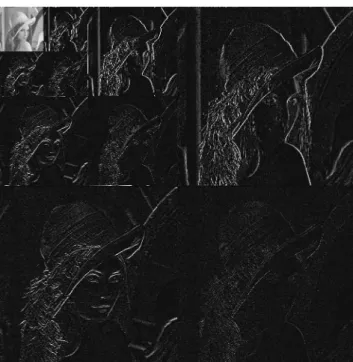
An example of a 2-D image, Lena, is presented to illus-trate the function of the ASQ algorithm mentioned before. The testbed images are of 512 512 pixels with 8-bit grey levels. Daubechies’ (1988, 1992) ® lter with length 20 is adopted in the DWT decomposition since it is orthogonal and compactly supported. A1represents

the lowest frequency subimage of the ® rst layer (resolu-tion1

2) DWT decomposition. Dh1, Dv1 and Dd1 are the

horizontal, vertical and diagonal oriented subimages with resolution 1

2, respectively. As a result, the 3-layer

DWT decomposition is derived and shown in ® gure 3, which reveals that the characteristic of self-similarity in the fractal would appear between scales with di€ erent resolutions. Therefore, Dh1 is regarded as the `domain

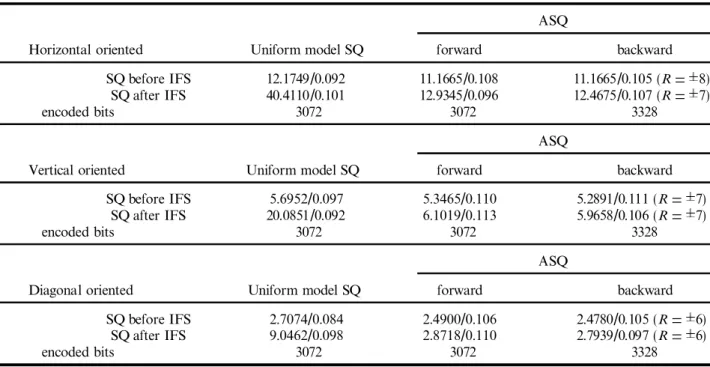
pool’ and Dh2 is considered to be the `range pool’. The improvement of mean squared error (MSE) on using the ® xed uniform model is listed in table 1. It reveals that the scalar quantizer: (i) must be placed in

front of the IFS algorithm to reduce the composite error, and more time is spent since every possible scale factor, while searching in IFS coding, should be quan-tized in advance; (ii) the ASQ with forward reconstruc-tion can perform well with no more bits being necessary to record, and the additional time used to execute the ASQ algorithm is acceptable; (iii) the backward recon-struction method can acheive the best MSE at the cost of increasing encoded bits and computing power. In practice, this reconstruction method is hard to use since some ASQ algorithms combining the IFS coding need to be checked to obtain the MSE better. This is a time-consuming task, especially in the IFS coding pro-cedures.

Next, we will show that the ASQ is superior to the uniform quantizer from the histogram point of view. The histogram of quantized data with a uniform model, as shown in ® gure 4(a), is uniformly spread on the dynamic range R. On the other hand, the histogram of quantization output with the ASQ algorithm in ® gure 4(b) is similar to that of scale factors without quantiza-tion in ® gure 2.

We also consider another version of the ASQ algor-ithm, which is more robust than the previous one since this method estimates the distribution by means of the Least Squared Error method instead of the prede® ned values of a and b. For the cases of R

₌

4 in table 2, the modi® ed ASQ algorithms perform well in robustness. Moreover, it also appears that the reconstruction MSE is highly related to the ratio of a/b. That is, the results would perform less successfully if the source is modi® ed inappropriately.

Figure 3. The image of Lena performed after the 3-layer DWT.

548 Bing-Fei Wu et al.

Table 2. The comparison of mean squared error in R

= ±

4 on ASQ and another version of ASQ with di€ erent values of a/b.In each

subimage, the minimum MSE is marked

w

. ASQ Dh2 ASQ a b 12 13 14 15 16 17 18 (LSE) MSE 11.1815 11.1993 11.3702 11.7887 12.2652 12.6266 13.0398 10.9594

w

ASQ Dh2 ASQ a b 12 13 14 15 16 17 18 (LSE) MSE 5.2800

w

5.3526 5.4554 5.6068 5.7122 5.7918 5.8808 5.3677 ASQ Dh2 ASQ a b 12 13 14 15 16 17 18 (LSE) MSE 2.4712

w

2.4780 2.4838 2.5120 2.5468 2.5884 2.6150 2.5201

Figure 4. The histograms of the quantized output: (a) uniform mnodel and (b) ASQ algorithm with a

=

1, b

=

5 and R

=

8. Table 1. The comparison of mean squared error and execution time on uniform model `before’ and `after’ IFS coding, and the ASQ

algorithm with di€ erent reconstruction modes: forward and backward. a

=

1, b

=

5, default dynamic range R

= ±

8.

ASQ

Horizontal oriented Uniform model SQ forward backward

MSE SQ before IFS 12.1749/0.092 11.1665/0.108 11.1665/0.105 (R₌ 8)

/Time SQ after IFS 40.4110/0.101 12.9345/0.096 12.4675/0.107 (R₌ 7)

encoded bits 3072 3072 3328

ASQ

Vertical oriented Uniform model SQ forward backward

MSE SQ before IFS 5.6952/0.097 5.3465/0.110 5.2891/0.111 (R₌ 7)

/Time SQ after IFS 20.0851/0.092 6.1019/0.113 5.9658/0.106 (R₌ 7)

encoded bits 3072 3072 3328

ASQ

Diagonal oriented Uniform model SQ forward backward

MSE SQ before IFS 2.7074/0.084 2.4900/0.106 2.4780/0.105 (R₌ 6)

/Time SQ after IFS 9.0462/0.098 2.8718/0.110 2.7939/0.097 (R₌ 6)

encoded bits 3072 3072 3328

5. Conclusion

We have proposed the adaptive self-quantizer to solve the quantization problem of scale factors in wavelet-based fractal image compression. In source modelling, we introduced the Least Squared Error method to esti-mate recursively the probability density function at the values of decision levels. Therefore, the distribution can be obtained by interpolating the estimated density func-tions linearly. The quantizer has the funcfunc-tions of adap-tivity and self-adjustment. In addition, it introduces the optimal sense in adapting the reconstruction levels of the quantizer such that we can reduce the quantization error generated by a ® xed uniform model.

Acknowledgments

This work was supported by National Science Council under Grant NSC87-2213-E-009-043.

References

Antonini, M., Barlaud, M., Mathieu, P., and Daubechies, I.,

1992, Image coding using wavelet transform. IEEE Transactions

on Image Processing,1, 205± 220.

Barnsley, M. F., andJacquin, A.,1988, Application of recurrent iterated function systems to images. Proceedings SPIE,1001, 122± 131.

Chan, C., andVetterli, M.,1995, Lossy compression of individual signals based on string matching and one pass codebook design. In

Proceedings ICASSP’95, Detroit, MI, pp. 2491± 2494.

Crisafulli, S, and Bitmead, R. B., 1993, Adaptive quantization: Solution via nonadaptive linear control. IEEE Transactions on

Communication,41, 741± 748.

Davis, G. M., 1995, Self-quantization of wavelet subtree in

Proceedings SPIE, Wavelet Applications II, Orlando. Edited by

H. H. Szu,2491, 141± 152.

Daubechies, I., 1988, Orthonormal bases of compactly supported wavelets. Communications on Pure and Applied Mathematics, 41, 906± 966; 1992, Ten L ectures on Wavelets (Philadelphia, PA: SIAM).

Fisher, Y., 1994, Fractal Compression: Theory and Application to

Digital Images (New York: Springer Verlag).

Goodwin, G. C., andSin, K. S.,1984, Adaptive Filtering Prediction

and Control (Englewood Cli€ s, New Jersey: Prentice-Hall).

Hang, H.-M., and Woods, J. W., 1995, Handbook of Visual

Communications. (San Diego: Academic Press).

Hsu, H.-H., Hu, Y.-Q., andWu, B.-F.,1998, An integrated method in wavelet-based image compression, The Journal of the Franklin

Institute,335B, 1053± 1068.

Jacobs, E. W., Fisher, Y., andBoss, R. D.,1992, Image compression: a study of the iteratied transform method. Signal Proceeding,29, 251± 263.

Jacquin, A. E.,1993, Fractal image coding: a review. Proceedings of

the IEEE,81, 1451± 1465.

Jayant, N. S.,1973, Adaptive quantization with a one-word memory.

Bell Systems Technology Journal,52, 1119± 1144.

Mallat, S. G.,1989, A theory for multiresolution signal decomposi-tion: the wavelet representation. IEEE Transactions on Pattern

Analysis and Machine Intelligence,11, 674± 693.

Max, J.,1960, Quantizing for minimum distortion. IRE Transactions

Information Theory,6, 7± 12.

Ortega, A., andVetterli, M.,1997, Adaptive scalar quantization without side information. IEEE Transactions Image Processing,6, 665± 676.

Rinaldo, R., andCalvagno, G.,1995, Image coding by block pre-diction of multiresolution subimages. IEEE Transactions on Image

Processing,4, 909± 920.

Steinberg, Y., andGutman, M.,1993, An algorithm for source cod-ing subject to a ® delity criterion, based on strcod-ing matchcod-ing. IEEE

Transactions on Information Theory,39, 877± 886.

Strang, G., and Nguyen, T., 1996, Wavelets and Filter Banks

(Cambridge, MA: Wellesley-Cambridge).

Vetterli, M, and KovaCÏevicí, J., 1995, Wavelets and Subband Coding (Englewood Cli€ s, New Jersey: Prentice-Hall).

Widrow , B., andStearns, S. D.,1985, Adaptive Signal Processing (Englewood Cli€ s, New Jersey: Prentice-Hall).

Wu, B.-F., Hsu, H.-H., andHu, Y.-O.,1998, The global minimum of scalar quantization errors by discrete wavelet transforms in image compression, accepted by Proceedings of the National Science Council, Part A: Physical Science and Engineering.

Wu, B.-F., Hsu, H.-H., andHu, Y.-Q.,1997, Linear block prediction in wavelet-based fractal image compression. Submitted to Signal

Processing.