A generalized version space learning algorithm for noisy and uncertain data

A Generalized Version Space Learning

Algorithm for Noisy and Uncertain Data

Tzung-Pei Hong, Member, IEEE Computer Society, and Shian-Shyong Tseng, Member, IEEE Computer Society Abstract—This paper generalizes the learning strategy of version space to manage noisy and uncertain training data. A new learning algorithm is proposed that consists of two main phases: searching and pruning. The searching phase generates and collects possible candidates into a large set; the pruning phase then prunes this set according to various criteria to find a maximally consistent version space. When the training instances cannot completely be classified, the proposed learning algorithm can make a trade-off between including positive training instances and excluding negative ones according to the requirements of different application domains. Furthermore, suitable pruning parameters are chosen according to a given time limit, so the algorithm can also make a trade-off between time complexity and accuracy. The proposed learning algorithm is then a flexible and efficient induction method that makes the version space learning strategy more practical.

Index Terms—Machine learning, version space, multiple version spaces, noise, uncertainty, training instance.

———————— ✦ ————————

1

I

IN real applications of machine learning, data provided to learning systems by experts, teachers, or users usually contain wrong or uncertain information. Wrong and uncertain information will in general greatly influence the formation and use of the concepts derived [12], [18]. Modifying traditional learning methods so that they work well in noisy and uncertain environments is then very important.

Several successful learning strategies based on ID3 have been proposed [5], [14], [19], [20], [21]; most of these use tree-pruning techniques to cope with the problem of overfitting. As to version-space-based learning strategies, Mitchell proposed a multiple ver-sion space learning strategy for managing wrong information [15]. Hirsh handled wrong information by assuming attribute values had a known bounded inconsistency [9]. Antoniou [1], Carpineto [4], Haussler [8], Nicolas [17], and Utgoff [24] stu-died the influ-ence of the language bias on the inconsistency. Bundy et al. [3], Drastal et al. [7], Hong and Tseng [11], and Smirnov [23] modified the version space to learn disjunctive concepts. Genetic algorithms were applied to version space for getting better concepts by De Raedt and Bruynooghe [6] and Reynolds and Maletic [22]. Also, fuzzy learning methods were developed to derive fuzzy if-then rules so that wrong or ambiguous training data can be effectively processed [13], [25]. Other studies on this field are still in progress. In this paper, we propose a generalized version space learning algorithm to manage both noisy and uncertain data. The proposed learning algorithm can also easily make a trade-off between in-cluding positive training instances and exin-cluding negative ones according to requirements of learning problems. Furthermore, the

learning algorithm provides for a trade-off between computational time consumed and the accuracy of the final results by allowing users to assign appropriate values to two pruning factors in the learning process. When more computational time is used, the con-cept derived is more consistent with the data.

This new learning algorithm is more efficient than the multiple version spaces learning algorithm, and unlike Hirsh’s method, it does not require that we assume the error is bounded. Furthermore, the new method can process uncertain data. Time complexity is analyzed and experiments on the Iris Flower Problem confirm that our learning algorithm works as desired. The generalized version space learning strategy then improves the original version space learning strategy, making it more practical for real-world applications.

2

A G

V

S

L

S

This section proposes a generalized version space learning algorithm that provides more functions than the original learning algorithm. Sets S and G defined in the original version space learning algorithm are modified to provide these additional functions. In our method, the hypotheses in S/G no longer necessarily include/exclude all the positive/negative training instances presented so far, since noisy and uncertain data may be present. Instead, the most consistent i hypotheses are maintained in the S set and the most consistent j hypotheses are maintained in the G set (i and j are two parameters defined by the user). A numerical measure referred to as the count is attached to each hypothesis in S/G to summarize all posi-tive/negative information implicit in the training instances pre-sented so far. A hypothesis with a higher count in S includes more positive training instances; a hypothesis with a higher count in G excludes more negative training instances. The new sets S and G are then generalizations of the old sets, defined as follows:

S = {s|s is a hypothesis among the first i maximally consistent hypotheses. No other hypothesis in S exists which is both more specific than s and has equal or larger count}. G = {g|g is a hypothesis among the first j maximally consistent

hypotheses. No other hypothesis in G exists which is both more general than g and has equal or larger count}. The first i/j maximally consistent hypotheses in S/G, however, are not necessarily the ones with the largest i/j counts. A hypothe-sis in S that includes much positive information may possibly also include much negative information. Which hypotheses in S/G are the first i/j maximally consistent then depends on both sets S and G (and not only on S itself or on G itself).

For the proposed learning algorithm to make a trade-off be-tween including positive training instances and excluding nega-tive ones according to the requirements of specific learning prob-lems, a parameter called the factor of including positive instances (FIPI) is incorporated into the algorithm. The value of FIPI is 1 if the aim of the learning problem is only to include positive training instances and 0 if the problem aims only to exclude negative ones. The value of FIPI is usually between 0 and 1, depending on the need to include positive training instances and exclude negative ones. FIPI is 0.5 if including positive training instances and ex-cluding negative ones are of the same importance.

A number between −1 to 1 is used to represent the certainty of the classification of a training instance, as in the MYCIN [2] system. The certainty factor (or CF) of a training instance is 1 if the training instance definitely belongs to the positive class and −1 if the training instance definitely belongs to the negative class. Otherwise, CF is assigned a value between −1 and 1 according to the certainty with which a training instance is judged to belong to the positive class.

Once a certainty factor is attached to each training instance to represent its uncertainty, each training instance can be thought of as partially positive and partially negative. Hence sets S and G

1041-4347/97/$10.00 © 1997 IEEE

————————————————

• T.-P. Hong is with the Department of Information Management,

Kaohsi-ung Polytechnic Institute, KaohsiKaohsi-ung County, Taiwan, 84008. E-mail: tphong@nas05.kpi.edu.tw.

• S.-S. Tseng is with the Department of Computer and Information Science,

National Chiao-Tung University, Hsinchu, Taiwan, 30050, Republic of China. E-mail: sstseng@cis.nctu.edu.tw.

Manuscript received Apr. 18, 1995.

For information on obtaining reprints of this article, please send e-mail to: transkde@computer.org, and reference IEEECS Log Number K96089.

INPUT: A set of n training instances, each with uncertainty CF, the value of the parameter FIPI, and the maxi-mum numbers i, j of the hypotheses maintained in S and G.

OUTPUT: The hypotheses in sets S and G that are maximally consistent with the training instances.

STEP 1: Initialize S to contain only the most specific hy-pothesis f with count = 0 and initialize G to con-tain only the most general hypothesis with count = 0 in the whole hypothesis space.

STEP 2: For each newly presented training instance with uncertainty CF, do STEP 3 to STEP 7.

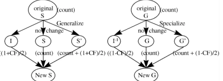
STEP 3: Generalize/Specialize each hypothesis with count = ck in S/G to include/exclude the new traing in-stance; attach new count ck + (1 + CF)/2/ ck + (1 − CF)/2 to each newly formed hypothesis in S/G; call the newly formed set S′/G′ for convenience. STEP 4: Find the set S”/G” including/excluding only the

new training instance itself, and set the count of each hypothesis in S”/G” to be (1 + CF)/2/ (1 − CF)/2. STEP 5: Combine the original S/G, S′/G′, and S”/G”

to-gether to form a new S/G (Fig. 1). If identical hypotheses with different counts are present in the combined set, only the hypothesis with the maximum count is retained. If a particular hy-pothesis is both more general/specific than an-other and has an equal or smaller count, discard that hypothesis.

STEP 6: For each hypothesis s/g with count cs/cg in the new S/G, find the hypothesis g/s in the new G/S that is more general/specific than s/g and has the maximum value of count cg/cs. Calculate the con-fidence as FIPI × cs + (1 − FIPI) × cg.

STEP 7: Retain the hypotheses with the first i/j highest confidence in the new S/G and discard the others.

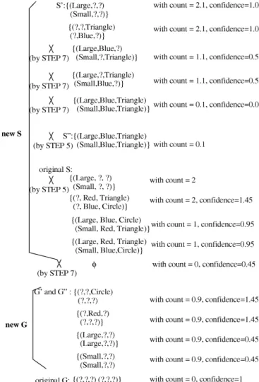
Assume each training instance can be described as an unordered pair of simple objects characterized by three nominal attributes [16]. Each object is described by its shape (e.g., circle, triangle), its color (e.g., red, blue), and its size (e.g., large, small). Assume the following three uncertain training instances are presented:

Instance 1. {(Large Red Triangle) (Small Blue Circle)} with CF = 1, Instance 2. {(Large Blue Circle) (Small Red Triangle)} with CF = 1, Instance 3. {(Large Blue Triangle) (Small Blue Triangle)} with CF =

−0.8.

Also assume FIPI is 0.5, i is 5, and j is 5. The process of manag-ing Instances 1 and 2 is shown in Fig. 2 (confidence is not shown here), and the process for managing instance 3 is shown in Fig. 3.

The most promising version space is bounded by the hypo-thesis {(? Red Triangle) (? Blue Circle)} in S and the hypotheses {(? ? Circle) (? ? ?)} and {(? Red ?) (? ? ?)} in G.

4

T

C

The time complexity of the generalized version space learning algorithm is analyzed in this section. The following basic unit of processing time will be used:

D

Also define kg as the maximum number of possible ways to specialize a hypothesis to exclude a training instance, and define ks as the maximum number of possible ways to generalize a hy-pothesis to include a training instance. For the learning algorithm proposed in Section 2, the processing time includes the required specialization/generalization processes and checking. Checking is used for examination of redundancy, subsumption, and contra-diction between hypotheses in sets S and G. Checking between any two hypotheses can be finished within a unit operation

cause it is simpler than generating a hypothesis to include a train-ing instance or to exclude a traintrain-ing instance.

Let T(n) denote the time complexity of our generalized version space learning algorithm in dealing with n training instances. The time complexity of each step is listed in Table 1.

Therefore, T(n) = O(1) +

n * (O(i * k_s + j * k_g) + O(k_s + k_g) + O((i * k_s)2 + (j * k_g)2) + O((i * ks) * (j * kg)) + O(i 2 * ks + j 2 *kg)) + O(1) = n * (O((i * ks) 2 + (j * kg) 2 + (i * ks) * (j * kg)) = O(n * ((i * k_s)2 + (j * k_g)2 + (i * k_s) * (j * k_g)).

There are usually more possible ways to exclude a training in-stance from a hypothesis than to include a training inin-stance in a hypothesis, so k_g is usually larger than k_s. This also implies that j must be set larger than i for the generalized version space learning algorithm to have good accuracy. For this case, the time complex-ity can be reduced as follows:

T(n) = O(n * (j * kg)) 2

.

For a given learning problem, kg is a constant. The time com-plexity can then be further reduced as follows:

T(n) = O(n * j) 2.

5

E

To demonstrate the effectiveness of the proposed generalized ver-sion space learning algorithm, we used it to classify Fisher’s Iris Data. There are three species of iris flowers to be distinguished: se-tosa, versicolor, and verginica. There are 50 training instances for each class. When the concept of setosa is learned, training instances belonging to setosa are considered to be positive; training instances belonging to the other two classes are considered to be negative.

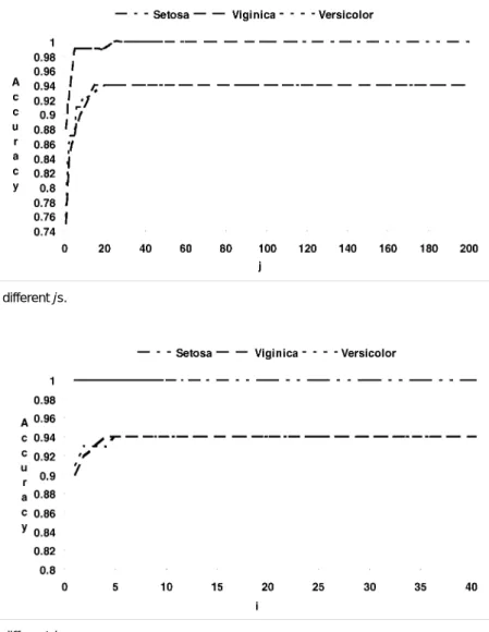
The generalized version space learning algorithm was imple-mented in C language on an IBM PC/AT. The algorithm was run 100 times, using different random partitions of the sample set. The average classification rates for the three kinds of iris flowers are

shown in Fig. 4 for i = 10 and different js and in Fig. 5 for j = 25 and different is.

Figs. 4 and 5 show that the classification accuracy increases as i and j increase. Also, j must be set larger than i for the generalized Fig. 2. Learning results for Instances 1 and 2.

Fig. 3. Learning results for Instance 3.

TABLE 1

TIME COMPLEXITY IN THE GENERALIZED VERSION SPACE LEARNING ALGORITHM

version space learning algorithm to have good accuracy, since there are usually more possible ways to exclude a training instance from a hypothesis than there are to include a training instance in a hy-pothesis. For the Iris Flower Learning Problem, the classification accuracy converges to 1 for setosa, 0.94 for versicolor, and 0.94 for verginica when i ³ 5 and j ³ 25. Our method is as accurate (96% in average) as Hirsh’s IVSM (96%) [9], even though our method does not assume knowledge of the bounded inconsistency is available. The time complexity of IVSM however depends on the number of nearby instances and the maximum possible numbers of hypothe-ses in both boundary sets [9], but not on the predefined i and j.

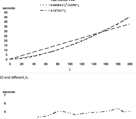
Experiments were also conducted to determine the execution time of the generalized version space learning algorithm for dif-ferent is and js. Results are shown in Fig. 6 for i = 10 and difdif-ferent js and in Fig. 7 for j = 10 and different is.

In Fig. 6, the execution time is approximately propor-tional to O(j2). In Fig. 7, the execution time converges to a constant (approximately 5 seconds) for j = 10 and i ³ 60. These results are quite consistent with the time complexity analysis in Section 4.

6

C

We have proposed a generalized version space learning algorithm that can manage both noisy and uncertain training instances and find a maximally consistent version space. The parameter FIPI in the proposed learning algorithm can be adjusted so that the

algo-rithm makes a trade-off between including positive training in-stances and excluding negative ones according to the requirements of different application domains. Furthermore, suitable i and j can be chosen according to a given time limit, so that the algorithm makes a trade-off between time-complexity and accuracy. The time complexity is analyzed to be O(j2). Finally, experimental re-sults on Iris data are consistent with the theoretical analysis. Ex-perimental results also show that our method yields a high accu-racy. The proposed learning algorithm is then a flexible and effi-cient induction method.

A

The authors would like to thank the anonymous referees for their very constructive comments. This research was supported by the National Science Council of the Republic of China under contract NSC84-2213-E214-13.

R

[1] G. Antoniou, “Version Space Algorithms on Hierarchies with Exceptions,” Proc. Sixth Portuguese Conf. AI, pp. 136-149, 1993. [2] B.G. Buchanan and E.H. Shortliffe, Rule-Based Expert Systems}The

MYCIN Experiments of the Stanford Heuristic Programming Project.

Reading, Mass.: Addison-Wesley, 1984.

[3] A. Bundy, B. Silver, and D. Plummer, “An Analytical Comparison of Some Rule-Learning Programs,” Artificial Intelligence, vol. 27, pp. 137-181, 1985.

Fig. 4. Accuracy for i = 10 and different js.

[4] C. Carpineto, “Shift of Bias without Operators,” Proc. 10th

Euro-pean Conf. Artificial Intelligence, pp. 471-473, 1992.

[5] P. Clark and T. Niblett, “The CN2 Induction Algorithm,” Machine

Learning, vol. 3, pp. 261-283, 1989.

[6] L. De Raedt and M. Bruynooghe, “A Unifying Framework for Concept-Learning Algorithms,” Knowledge Engineering Rev., vol. 7, no. 3, pp. 251-269, 1992.

[7] G. Drastal, R. Meunier, and S. Raatz, “Error Correction in Con-structive Induction,” Proc. Sixth Int’l Workshop Machine Learning, pp. 81-83, 1989.

[8] D. Haussler, “Quantifying Inductive Bias: AI Learning Algo-rithms and Valiant’s Learning Framework,” Artificial Intelligence, vol. 36, pp. 177-221, 1988.

[9] H. Hirth, “Generalizing Version Space,” Machine Learning, vol. 17, pp. 5-46, 1994.

[10] T.P. Hong, “A Study of Parallel Processing and Noise Manage-ment on Machine Learning,” PhD thesis, National Chiao-Tung Univ., Taiwan, 1991.

[11] T.P. Hong and S.S. Tseng, “Splitting and Merging: An Approach to Disjunctive Concept Acquisition,” Proc. IEEE Int’l Workshop

Emerging Technologies and Factory Automation, pp. 201-205, 1992.

[12] Y. Kodratoff, M.V. Manago, and J. Blythe, “Generalization and Noise,” Int’l J. Man Machine Studies, vol. 27, pp. 181-204, 1987. [13] C.C. Lee, “Fuzzy Logic in Control Systems: Fuzzy Logic

Control-ler}Part I and Part II,” IEEE Trans. Systems, Man, and Cybernetics, vol. 20, no. 2, pp. 404-435, 1990.

[14] J. Mingers, “An Empirical Comparison of Pruning Methods for Decision Tree Induction,” Machine Learning, vol. 4, pp. 227-243, 1989.

[15] T.M. Mitchell, “Version Spaces: An Approach to Concept Learn-ing,“ PhD thesis, Stanford Univ., Stanford, Calif., 1978.

[16] T.M. Mitchell, “Generalization as Search,” Artificial Intelligence, vol. 18, pp. 203-226, 1982.

[17] J. Nicolas, “Empirical Bias for Version Space,” Proc. Int’l Joint

Conf. AI, pp. 671-676, 1991.

[18] J.R. Quinlan, “The Effect of Noise on Concept Learning,” Machine

Learning: An Artificial Intelligence Approach, R.S. Michalski, J.G.

Carbonell, and T.M. Mitchell, eds., vol. 2. Palo Alto, Calif.: Toiga, pp. 149-166, 1984.

[19] J.R. Quinlan, “Simplifying Decision Trees,” Int’l J. Man-Machine

Studies, vol. 27, pp. 221-234, 1987.

[20] J.R. Quinlan, “Unknown Attribute Values in Induction,” Proc.

Sixth Int’l Machine Learning Workshop, pp. 164-168, 1989.

[21] J.R. Quinlan, C4.5 Programs for Machine Learning. San Mateo, Calif.: Morgan Kaufmann, 1992.

[22] R.G. Reynolds and J.I. Maletic, “The Use of Version Space Con-trolled Genetic Algorithms to Solve the Boole Problem,” Int’l J.

Artificial Intelligence Tools, vol. 2, no. 2, pp. 219-234, 1993.

[23] E.N. Smirnov, “Space Fragmenting}A Method for Disjunctive Concept Acquisition,” Proc. Fifth Int’l Conf. Artificial Intelligence:

Methodology, Systems, and Application, pp. 97-104, 1992.

[24] P.E. Utgoff, Machine Learning of Inductive Bias. Boston: Kluwer, 1986.

[25] L.X. Wang and J. M. Mendel, “Generating Fuzzy Rules by Learn-ing from Examples,” Proc. IEEE Conf. Fuzzy Systems, pp. 203-210, 1992.

Fig. 6. Execution time for i = 10 and different js.